Superdiffusion of massive particles induced by multi-scale velocity fields

Abstract

We study drag-induced diffusion of massive particles in scale-free velocity fields, where superdiffusive behavior emerges due to the scale-free size distribution of the vortices of the underlying velocity field. The results show qualitative resemblance to what is observed in fluid systems, namely the diffusive exponent for the mean square separation of pairs of particles and the preferential concentration of the particles, both as a function of the response time.

1 Introduction

Understanding how complex flows advect massive particles is a challenging problem not only when addressing natural phenomena like rain drop formation [1] and protoplanetary disks [2], but also for environmental and industrial applications such as dispersion of pollutants [3] and design of the combustion chamber in engines [4].

During the advection of massive particles by the flow, different transport mechanisms come into play such as the dissipative dynamics of trajectory attractors and the ejection of the particles from the vortices (eddies) by centrifugal forces. The interplay of these mechanisms, when driven by the multi-scale vortical dynamics of turbulent flows, leads to classical empirical features such as superdiffusion [5] and preferential concentration (PC) [6].

Experimental and computational studies show that advection of particles by turbulent flows is generally a superdiffusive process, that is, the mean squared separation of the particles $\langle R^{2}\rangle$ grows faster than $t$, the first power of time [7]. An early empirical study by Richardson [8] suggested that the mean squared separation of elements of carrier fluid itself grows with $t^{3}$.

However, preferential concentrations only occur when the density of particles differs from that of the carrier flow. The regions of high vorticity act on the heavier particles like centrifuges pushing them toward regions of low vorticity and high strains while trapping lighter particles [6] which leads to clustering of particles and inhomogeneity in their distribution.

Experimental difficulties in measuring Lagrangian quantities and limitations of the numerical simulations in resolving a wide range of scales of flow motion have posed major obstacles in study of these processes [9]. During the last decades, great progresses, experimental and computational, have been made in overcoming these obstacles (see Ref. [10, 11] for two recent reviews).

Attempts have been made in using toy models to separate and study the mechanisms present in real turbulent flows. Bec et al. [12] introduced a simple flow model to study the role of ejection of particles by eddies in the distribution of massive particles. The model consists of a grid of two-dimensional cells with high vorticities which eject particles with a rate depending on the response time of the particles to the flow. Their results for the mass probability distribution in the fully mixed state show qualitative agreement with what is observed in real systems. However, they do not address the problem of existence of superdiffusive regimes. Moreover, the model lacks a multi-scale vortical structure, a dominant feature in real turbulent flows, which indeed turns out to be responsible for superdiffusive behaviors.

In this Letter, we introduce a heuristic model for two dimensional scale-free velocity fields which incorporates a multi-scale vortical structure, to study the role of ejection of particles by eddies, separated from other mechanisms such as dissipation. Here, we show that the multi-scale structure is a key feature responsible for superdiffusion regimes in the transport of massive particles. In addition, within the limitations of the model, the results obtained show qualitative resemblance to what is observed in real systems. In particular, we discuss the applicability of the results to the problem of preferential concentration and Richardson’s law.

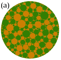
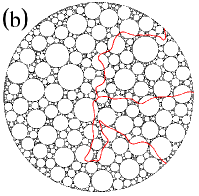
Figure 1: (Color Online). (a) Modelling multi-scale velocity fields, using rigid discs to represent vortices (eddies) of different sizes. Each eddy has a fixed center and rotates clockwise (green) or counter-clockwise, in order to ensure absence of sliding at the contact points. (b) Trajectories of three massive particles when particles follow Stokes drag (see Eq. (1)).

2 Bearings as models for velocity fields

Our model for the velocity field of the flow is based on random polydisperse packings of discs fulfilling the particular condition of all discs being able to rotate simultaneously without sliding on each other at their contact points. At their contact points all discs have the same tangential velocity $v_{0}$ in order not to have frustration. Therefore, $v_{0}$ is a global parameter of the system while the angular velocity of disc $i$ is inversely proportional to its size, $v_{0}=\omega_{i}R_{i}$.

Figure 1a represents such a random packing where colors indicate the sign of the angular velocity of the discs. One notes that no two discs which are in contact will have the same color since they rotate in opposite directions. Such bichromatic packings are referred to as bearings and were originally introduced in the field of granular materials as a geometrical explanation of seismic gaps in tectonic plates [13, 14, 15].

Random bearings used here are constructed by directly imposing the bichromacy condition. Initially a number of discs of random sizes are distributed randomly in the system. To each disc one color or the other is assigned randomly. The rest of the space is filled by inserting the largest possible discs with colors chosen such that no two discs of the same color touch each other .

The configurations are complete (space-filling), self-similar and contain some level of randomness introduced by the initialization and the choice of parameters in the construction procedure (see Refs. [16, 14, 15] for more details.) Following Mandelbrot [17] one can define the Hausdorff-dimension of the void space, which is related to the exponent of the size distribution of the discs. In practice, a lower cut-off on the size of the vortices is inevitable, leading to a limited range of scales defined as $r_{M}/r_{m}$.

In this context, we regard each rotating disc as a vortex with a linear velocity profile inside, that is, the fluid in each disc is moving in the same way as if it were a rigid body. In this way, we obtain a velocity field containing eddies of many different scales. Although, the statistical properties of such a flow field do not necessarily coincide with those of real turbulent flows, its energy spectrum follows a power-law whose exponent is directly related to the exponent of the size distribution of the eddies (see Ref. [13]). During their rotation, the centers of the eddies are kept fixed which makes the velocity field stationary.

The particle-flow interaction depends on the shape of the particles and the difference between their density and that of the fluid [18]. Here, we will consider particles much denser than the carrier fluid. Neglecting buoyancy and considering small particle Reynolds numbers, when the size of the particles is much smaller than any active scale of the flow, the force exerted on the particles by the flow follows Stokes drag:

$$\frac{d\vec{V}_{p}}{dt}=\frac{\vec{V}_{f}-\vec{V}_{p}}{\tau},$$ (1)

where $\tau$ is the response time of the particles and $V_{f}$ and $V_{p}$ are the velocities of the flow and the particle, respectively. For a single vortex we have $\vec{V_{f}}=w\hat{z}\times(\vec{r}-\vec{r_{c}})$, where $\vec{r}$ and $\vec{r}_{c}$ denote the position of the particle and the center of the vortex, respectively, and $\hat{z}$ is the unit vector perpendicular to the vortex. Equation (1) is solved analytically to obtain particle trajectories. Figure 1b shows three typical trajectories of particles through the system of eddies.

Inside the voids between eddies, we assume in Eq. (1) two different cases, namely, ballistic ($\vec{V_{f}}=\vec{V_{p}}$) and damping ($\vec{V_{f}}=0$). By assuming ballistic trajectories in the voids, we exclude all dissipation in the flow field. In the damped case the particles are slowed down which corresponds to a loss of energy and represents viscous dissipation on the scale of the smallest eddy, i.e.  the Reynolds cut-off.

As the control parameter for flow-particle interaction, the Stokes number $S$ is often used instead of the response time $\tau$. It is dimensionless and related to $\tau$ through the following relation:

$$S=\frac{\tau}{\tau_{c}},$$ (2)

where $\tau_{c}$ is a characteristic time of the system. However, since there is no unique characteristic time in our system we use $\tau$ in our simulations for parameterizing the flow-particle interaction.

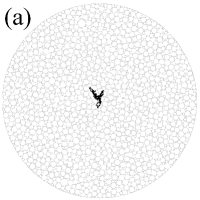
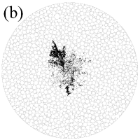
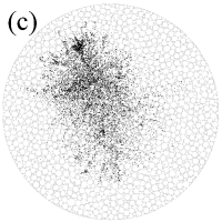
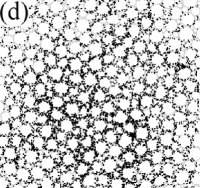
Figure 2: Different stages during the diffusion of $10^{4}$ particles: (a) $\tau=14$, $t=2$, (b) $\tau=14$, $t=6$, (c) $\tau=14$, $t=10$. (d) $\tau=0.01$, $t=3$. The velocity field is defined through $1.6\times 10^{4}$ vortices embedded in a circular space of unit size (shown in the background) where the centers of the vortex stay fixed in time. The size of the vortices varies from $r_{M}=0.02$ down to $r_{m}=10^{-4}$ in units of system size ($r_{M}/r_{m}=200$).

3 Superdiffusion and preferential concentration

Having set up the velocity field as described above, a total number of $10^{4}$ particles are released in a small region in the center of the system with very small initial velocity in randomly chosen directions. Figure 2a, 2b, and 2c represent, respectively, the early, intermediate and final stages for one specific configuration with a moderate value of $\tau$. Figure 2d shows the final stage for a very small value of $\tau$ and here the preferential concentration becomes visible.

To improve the statistics, we average the results over $50$ different eddy configurations, where the cut-off of the eddy size is $r_{m}=10^{-4}$, and the maximum size is $r_{M}=0.02$ in units of the system diameter. In analogy to turbulence, the range of spatial scales between the sizes of the smallest and the largest discs will be here referred to as inertial range. In the simulations, the particles which reach the boundary of the system are removed permanently. In order to prevent this from affecting the results, we gaurantee reaching the mixed state before a signifacant number of particles has left the system by choosing the size of the largest eddies to be much smaller than the system size.

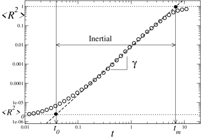
Figure 3: Mean square separation $\langle R^{2}\rangle$ between two particles as function of time $t$ for a specific response time $\tau=3$. Distances are in units of the system size $L$, the radius of the circular space, and time is in units of $L/v_{0}$, where $v_{0}$ is the tangent velocity of the discs. The two times $t_{0}$ and $t_{m}$ delimit the interval within which particles are in the inertial regime (see text). Time $t_{0}$ marks the beginning of the inertial regime whereas beyond $t_{m}$ particles are uniformly distributed in the system ($\langle R^{2}\rangle\sim 1$). The dashed line has slope $\gamma$ and its intersection with the dotted lines enables one to derive $t_{0}$ and $t_{m}$ (see text).

Figure 3 shows the mean square pair distance $\langle R^{2}\rangle$ between two particles as function of time. The initial regime (dotted line) for very short times, $t\leq t_{0}$, corresponds to the period when the particles have not yet penetrated into the eddies of different scales. For large times, $t\geq t_{m}$, particles either escape or spread uniformly throughout the system yielding $\langle R^{2}\rangle\sim L^{2}$, as indicated by the horizontal dotted line, where $L=1$ is the radius of the system. In the intermediate regimes, $t_{0}\leq t\leq t_{m}$, where particles are still in the inertial range, one observes $\langle R^{2}\rangle\sim t^{\gamma}$, since these are regimes where the multi-scale structure of the flow is dominant. These regimes are limited to times when the particles have not yet gone through scales much larger than the size of the largest eddies. This behavior is qualitatively similar to that of observed for separation of fluid particles via direct numerical simulations Ref. [19].

The values for $\gamma$, $t_{0}$ and $t_{m}$ depend on the response time $\tau$, and are found using a power-law fit to $\langle R^{2}\rangle$ in the inertial range $[t_{0},t_{m}]$, which can be written in the following form,

$$\langle R^{2}\rangle=\langle R^{2}\rangle_{0}\left(\frac{t}{t_{0}}\right)^{\gamma}$$ (3)

where $\langle R^{2}\rangle_{0}$ denotes the mean square separation of the particles before entering the inertial range.

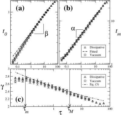
Figure 4: (a) The transient time $t_{0}$ as a function of $\tau$ together with (b) the mixing time $t_{m}$ and (c) the exponent $\gamma$. Fits in (a) and (b) yield power-laws, namely $t_{0}\sim\tau^{\beta}$ and $t_{m}\sim\tau^{\alpha}$ (see text). In (c) the dashed line indicates $\gamma$ in Eq. (4) where $a=-6$, $b=2.38$ and $\delta=0.101$.

As shown in Figs. 4a and 4b, $t_{0}$ and $t_{m}$ behave as power-laws of $\tau$, namely $t_{0}=B\tau^{\beta}$ and $t_{m}=A\tau^{\alpha}$ respectively, independently of having dissipative voids or vacuum. The fit beyond $\tau$ (dashed lines) yields, $A=4.7\pm 1.2$, $\alpha=0.44\pm 0.14$, $B=0.437\pm 0.005$ and $\beta=0.303\pm 0.005$. The value for $\log{\langle R^{2}\rangle_{0}}=\gamma\log{(t_{0}/t_{m})}\simeq 10^{-6}$ does not depend on $\tau$ but only on the specific initialization of the system. Thus, from Eq. (3) we can write $\gamma$ as a function of $\tau$,

$$\gamma=\frac{a}{b+\delta\log{\tau}}$$ (4)

with $a=\log{\langle R^{2}\rangle_{0}}$, $b=\log{(B/A)}$ and $\delta=\beta-\alpha$. Figure 4c plots $\gamma$ as a function of $\tau$ (symbols) comparing it with Eq. (4) (dashed line) which fits the observed values of $\gamma$ in the middle range of the $\tau$-spectrum, approximately at $\tau_{1}<\tau<\tau_{2}$. The deviations from Eq. (4) imply that $t_{0}$ and $t_{m}$ obey a power-law only for the intermediate and not for the limiting values of $\tau$ which is what one should expect; (i) when $\tau\to\infty$, particles’ inertia is very large and therefore they travel ballistically through the system without being significantly deflected by the flow, yielding $\gamma\to 2$, (ii) when $\tau\to 0$, which characterizes tracers (fluid particles), the motion of the particles follows Richardson’s law $\langle R^{2}\rangle\propto t^{3}$ [8]. Although the original Richardson’s experiment was in three dimensions it can be shown that Richardson’s law is independent of the dimensionality of the system [19].

These observations raise the hypothesis that the main ingredient underlying Richardson’s law is the multi-scale structure of vortices with the dissipative dynamics playing a minor role. However, this cannot be rigorously verified due to the limitations of the model. As mentioned before, our velocity fields are stationary and lack the sweeping effect. Therefore, the particles become trapped in local eddies in the limit of $\tau=0$ and cannot disperse.

In the second part of our study, we provide an estimate of the range of $\tau$, $(\tau_{1},\tau_{2})$, showing that the effect of the limitations of the model is minor. This interval is also shown in Fig. 4c.

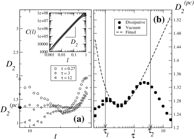
Figure 5: (a) The correlation dimension $D_{2}$ as a function of time for three values of $\tau$. The inset shows how $D_{2}$ is determined: at each instant $t$, one computes the average number $C(l)$ of pairs of particles that are closer than a distance $l$; this yields a power-law $C(l)\sim l^{D_{2}}$. At intermediate times $D_{2}$ attains a minimum (dashed line) which indicates maximal preferential concentration $D_{2}^{(pc)}$ (see text). (b) The correlation dimension $D_{2}^{(pc)}$ when maximum preferential concentration is attained in the inertial range. The dashed curve fitting $D_{2}^{(pc)}$ in the range $\tau_{1}<\tau<\tau_{2}$ resembles the behavior found with DNS calculations of particles in homogeneous turbulent flows[20] (see text).

Let us next examine the occurrence and properties of preferential concentrations. To quantify the degree of preferential concentration we use the correlation dimension as also used by other authors [20], defined as [21, 22]:

$$D_{2}=\lim_{l\rightarrow 0}\frac{d(\log{C(l)})}{d(\log{l})},$$ (5)

where $C(l)$ is the fraction of pairs of particles separated by a distance smaller than $l$. This quantity takes on the value zero, one and two when particles are all clustered in a single point, on a line, and uniformly distributed over the space, respectively. As can be seen from the inset of Fig. 5a, in our case $C(l)\sim l^{D_{2}}$, which defines an effective exponent $D_{2}$ for each instant $t$.

Figure 5a shows the evolution of $D_{2}$ in time for three values of $\tau$. For initial times, the correlation dimension depends strongly on the initial condition. For very large times, one observes that $D_{2}$ converges to the dimension of the system itself ($D_{2}=2$), i.e. particles distribute homogeneously throughout the system. For intermediate times, one observes a local minimum (dashed line), which implies that preferential concentration is maximal. For larger systems, we observe that the plateau where $D_{2}=D_{2}^{(pc)}$ becomes broader (not shown). Therefore, we regard $=D_{2}^{(pc)}$ as the characteristic value of the correlation dimension. While the results shown here are for the case of empty (ballistic) voids, similar results are obtained when the voids are dissipative.

Figure 5b shows $D_{2}^{(pc)}$ as a function of $\tau$. Within the range $\tau_{1}<\tau<\tau_{2}$ one finds a behavior (dashed line) consistent to what is known for the correlation dimension in numerical experiments of heavy particles in turbulent fluids, namely for $\tau=0$ and $\tau\to\infty$ the correlation dimension converges to the dimension of the system (see Ref. [20]).

The deviations from such behavior observed outside the range $\tau_{1}<\tau<\tau_{2}$ are due to the finite range of scales of eddies. As mentioned before, the particles are initialized inside a small neighborhood moving in a randomly chosen direction. For large $\tau$ values ($\tau>\tau_{2}$), particle paths are approximately ballistic, moving apart from each other as a growing circle at large times which yields $D_{2}\sim 1$. For $\tau<\tau_{1}$, particle are approximately tracers and get quickly trapped in a circular trajectory inside one vortex. This last behavior is strengthened when voids are dissipative (bullets), since particles are trapped in the voids.

4 Conclusions

We introduced a two-dimensional heuristic model for multi-scale fluid velocity fields and studied the dependence of the drag-induced diffusion of massive particles on it. The model is based on discs of different sizes representing flow eddies which roll on each other without sliding. By computing the exponent of the mean squared displacement as a power-law of time we find superdiffusive regimes within a broad range of response times which is consistent with scaling analysis and with the particular limiting cases where Richardson’s law holds and also with the ballistic regime for heavy particles. The results show that the main feature responsible for the emergence of superdiffusion is the multi-scale vortical structure of the flow. We also find the characteristic footprint of preferential concentration as observed when particle disperse in turbulent flows, like for instance the plankton in the ocean. Being able to incorporate multi-scale features and at the same time separate distinct mechanisms for heavy particle dynamics in fluids, this model can be further extend to more general situations where, e.g. dissipation occurs inside the vortices.

- [1] \NamePeixoto J. Oort A. \BookPhysics of Climate \PublAmerican Institute of Physics, New York \Year1992
- [2] \NameI. de Pater J. Lissauer \BookPlanetary Science \PublCambridge Univ. Press, Cambridge \Year2001
- [3] \NameJ. Fan, K. Luon, Y. Zheng, H. Jin, K. Cen \ReviewPhys. Rev. E \Vol68, \Page036309 \Year2003
- [4] \NameWhite F. \BookFluid Mechanics \PublMcGraw-Hill, New York \Year2003
- [5] \NameG. M. Zaslavsky \ReviewPhys. Rep. \Vol371 \Page461 \Year2002
- [6] \NameEaton J. K. Fessler J. R. \ReviewInternational Journal of Multiphase Flow \Vol20 \Page169 \Year1994
- [7] \NameMonin A. Yaglom A. \BookStatistical Fluid Mechanics II \PublMIT Press, New York \Year1975
- [8] \NameRichardson L. F. \ReviewProc. R. Soc. London A \Vol110 \Page709 \Year1926
- [9] \NameFalkovich G., Gawedzki K., Vergassola M. \ReviewRev. Mod. Phys. \Vol73 \Page913 \Year2001
- [10] \NameToschi F. Bodenschatz E. \ReviewAnnual Review of Fluid Mechanics \Vol41 \Page375-404 \Year2009
- [11] \NameSalazar J. P.L.C. Collins L. R. \ReviewAnnual Review of Fluid Mechanics \Vol41 \Page405-432 \Year2009
- [12] \NameBec J. Chetrite R. \ReviewNew J. Phys. \Vol77 \Page1 \Year2007
- [13] \NameHerrmann H. J., Mantica G., Bessis D. \ReviewPhys. Rev. Lett. \Vol65 \Page3223 \Year1990
- [14] \NameBaram R. M., Herrmann H. J., Rivier N. \ReviewPhys. Rev. Lett. \Vol92 \Page044301 \Year2004
- [15] \NameBaram R. M. Herrmann H. J. \ReviewPhys. Rev. Lett. \Vol95 \Page224303 \Year2005
- [16] \NameLind P. G., Baram R. M., Herrmann H. J. \ReviewPhys. Rev. E. \Vol77 \Page021304 \Year2008
- [17] \NameMandelbrot B. B. \BookThe Fractal Geometry of Nature \PublFreeman, San Francisco \Year1982
- [18] \NameMaxey M. R. Riley J. J. \ReviewPhys. Fluids \Vol26 \Page883 \Year1983
- [19] \NameBoffetta G. Sokolov I. \ReviewPhys. Fluids \Vol14 \Page3224 \Year2002
- [20] \NameBec J., Biferale L., Cencini M., Lanotte A., Musacchio S., Toschi F. \ReviewPhys. Rev. Lett. \Vol98 \Page084502 \Year2007
- [21] \NameTang L., Wen F., Yang Y., Crowe C. T., Chung J. N., Troutt T. R. \ReviewPhys. Fluids A \Vol4 \Page2244 \Year1992
- [22] \NameP. Grassberger I. Procaccia \ReviewPhysica D \Vol9 \Page189 \Year1983