Phase diagram of a two-dimensional lattice gas model of a ramp system

Abstract

Using Monte Carlo Simulation and fundamental measure theory we study the phase diagram of a two-dimensional lattice gas model with a nearest neighbor hard core exclusion and a next-to-nearest neighbors finite repulsive interaction. The model presents two competing ranges of interaction and, in common with many experimental systems, exhibits a low density solid phase, which melts back to the fluid phase upon compression. The theoretical approach is found to provide a qualitatively correct picture of the phase diagram of our model system.

I Introduction

The presence of liquid-liquid (LL) equilibrium in simple fluids has drawn considerable attention in recent years,Katayama et al. (2000); Tanaka et al. (2004); Kurita and Tanaka (2005) mainly due to its connection with the existence of certain thermodynamic, structural and dynamic anomalies in liquid water.Tanaka (1996); Yamada et al. (2002); Brovchenko et al. (2005) The fact that there are significant regions of the phase diagram in which an increase of temperature at constant pressure is associated with a corresponding increase in density, or in which diffusivity is enhanced when the system is compressed, might be at first sight somewhat counterintuitive, and has therefore motivated a remarkable research effort. Most of the systems that exhibit this peculiar behavior are also known to present low density solid phases (with coordination numbers ranging from 2 to 5) less dense than their liquid counterparts. Melting upon compression is a common feature that has to be accounted for as well.

In this regard, simple models constitute a fundamental aid that can allow to identify those essential features key to the presence of the aforementioned anomalous behavior. Recent research has focused on two main categories of models: orientational and isotropic. The former class of models is constructed bearing in mind the orientational character of the hydrogen bond interaction or the strong directional character of the covalent bonding characteristic in systems with low density solid phases, such as silica,Saika-Voivod et al. (2000) germanium oxideSmith et al. (1995) or phosphorus.Katayama et al. (2000) For this class of materials, a series of realistic potentials have been employed in order to characterize their anomalies via computer simulation.Tanaka (1996); Yamada et al. (2002); Brovchenko et al. (2005); Sastry and Angell (2003); Ghiringhelli et al. (2004); Saika-Voivod et al. (2000) Useful as these studies might be, a better insight can be gained from simpler models which can be dealt with in some cases even analytically. Perhaps the precursor of the simple orientational models is the Bell-Lavis two-dimensional lattice model of water,Bell and Lavis (1970) recently somewhat extended by Barbosa and Henriques.Barbosa and Henriques (2008) In addition to these, the Mercedes Benz model of waterSilverstein et al. (1998), the 3D lattice gas model of Roberts and DebenedettiRoberts and Debenedetti (1996), and the two-dimensional associating lattice gas model of Henriques and BarbosaPRE_2005_71_031504 ; JCP_2009_130_184902 must also be mentioned.

The complexity of the above mentioned orientational models can be further reduced. A weighted orientational average from these types of interactions would lead in most cases to isotropic models with several interaction ranges. And, since the pioneering work of Hemmer and Stell,Hemmer and Stell (1970) it turns out that the presence of two competing scales or interaction ranges has been found to lie at the heart of the existence of multiple phase transitions in otherwise “simple” fluids . The ramp potential model proposed by Hemmer and Stell regained attention when JaglaJagla (1999) stressed the similarities between its behavior and the anomalous properties of liquid water. Since then, a good number of works have been devoted to the continuous ramp potential.Xu et al. (2005, 2006a, 2006b); Gibson and Wilding (2006); Caballero and Puertas (2006); Lomba et al. (2007) Other simple models with competing ranges of interaction, such as the hard-sphere square shoulder-square well potential have also been shown to exhibit LL equilibria.Skibinsky et al. (2004) But not only continuous models can furnish an illustrative qualitative picture of the phase behavior and various anomalies found in water and related systems. Isotropic lattice gas models have proven to be able to describe the qualitative features of these systems rather accurately. One dimensional,Bell (1969); Høye and Lomba (2008); hoye two dimensionalBalladares and Barbosa (2004) and three dimensionalhoye lattice gas models have been studied, using either mean field approaches, transfer matrix methods and/or computer simulation.

In this paper we will consider a two-dimensional lattice gas model closely connected with the one studied in Ref. hoye, in three dimensions. The model is characterized by two competing interaction ranges (a nearest neighbor hard core exclusion and a finite repulsive interaction on the next to nearest sites). This model is strongly related to the continuum shoulder model studied in Ref. Skibinsky et al., 2004, when the attractive interactions are absent. Our study will focus on the reentrant melting of the low density solid phase, using both computer simulation and Lattice Fundamental Measure Theory (LFMT).lafuente:2002b ; lafuente:2003a ; lafuente:2003b ; lafuente:2004 ; lafuente:2005 We will see how the theoretical approach provides a qualitatively fairly approximate picture of our model phase diagram.

The rest of the paper is sketched as follows. A brief description of the model is introduced in the next section. Section III is devoted to the simulation methodology. Details on the finite size scaling analysis of the transitions are included in Section IV. Section V describes the LFMT as applied to this model, and finally our most significant results and conclusions are presented in Section VI.

II Model

We consider a two-dimensional model defined on a triangular lattice. A given site of the lattice can be either empty or occupied by one particle. The occupation of that site excludes the occupation of its six nearest neighbor (NN) sites. In addition there is a repulsive interaction between pairs of particles located in pairs of sites that are next to nearest neighbors (NNN).

The potential energy of an acceptable configuration is then written as:

$${\cal U}=\epsilon\sum_{<ij>}n_{i}n_{j}.$$ (1)

where $<ij>$ indicates the set of NNN pairs of sites; the coordinates $n_{k}$ are equal to zero for empty sites and equal to one for occupied sites; and $\epsilon>0$.

In the limit of high temperature the interactions between NNN become negligible and the system behaves as a hard core lattice gas with NN exclusion. Such a model is the well known hard hexagon model, which exhibits a continuous order-disorder transition. The location of this transition was obtained by Baxter,JPAMG_1980_13_L61 ; baxter2 and it is believed to belong to the same universality class as the 3-state Potts model in two dimensions.RMP_1982_54_235 At high density the system adopts an ordered structure (that will henceforth be referred to as T3) in which the sites occupy preferentially one of the three sublattices of the system [see Fig. 1(a)], with a triangular structure. The density at close packing is $1/3$ (one third of the sites are occupied).

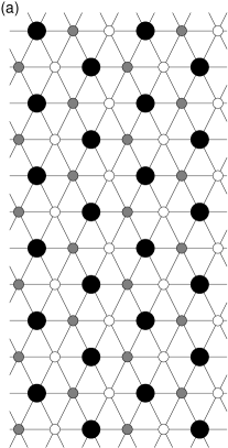
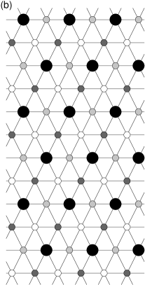
Figure 1: (a) Ordered structure at high temperature (large filled circles) and close packing. The three sublattices are identified by circles with different shading. Lines link nearest neighbor sites. The distance between nearest neighbors in each sublattice is $\sqrt{3}$, i.e. the distance to next nearest neighbors in the original lattice. (b) Low density ordered structure appearing at low temperature (large filled circles). The four sublattices are identified by circles with different shading. Lines link nearest neighbor sites. The distance between nearest neighbors in each sublattices is $2$, i.e. the distance to third neighbors in the original lattice. One fourth of the sites (large circles) of the lattice are occupied.

In the low temperature and low pressure limit (equivalently $\epsilon\to\infty$) another lattice hard core model is met. In this case an occupied site excludes the occupation of its NN and NNN. Under these exclusion rules, at high density we find again an ordered phase in which particles sit preferentially on one of the four corresponding sublattices [see Fig. 1(b)]. The close packing density is in this case $1/4$ (one fourth of the sites are occupied), and this ordered phase will henceforth be denoted T4. Attending to the symmetry of the order parameter and the dimensionality of the system, one expects to find an order-disorder transition belonging to the universality class of the 4-state Potts model in two dimensions.RMP_1982_54_235 Theoretical analysisPRB_1984_30_5339 and simulation resultsPRB_1989_39_2948 ; PRE_2008_78_031103 have shown that this transition is also continuous.

As in previous work by some of the authors,hoye we are interested in the phase transitions of the system at intermediate temperatures, where three phases: disordered, T4, and T3, can appear.

III Simulation methodology

In order to obtain the phase diagram of the system we have made use a number of Monte Carlo (MC) simulation techniques. At high temperature we have used a flat-histogram algorithm,hoye ; PRE_2005_71_046132 ; Lomba et al. (2007); JCP_2008_129_234504 inspired on the Wang-Landau (WL) method,PRL_2001_86_2050 ; PRE_2001_64_056101 to compute the Helmholtz energy function for all possible densities of the systems at fixed temperature and volume. In practice, the simulation procedure can be regarded as an extension of the MC simulation in the grand-canonical ensemble (GCE), in which the different number of particles are not weighted by a fixed chemical potential, but using a weighting function which permits us to extend the densities entering the sampling to an arbitrary range. Such a weighting function is not known a priori, but it can be computed following the strategies underlying the WL method. Once the Helmholtz energy function is known, for a given temperature, for all the densities and several system sizes, one can resort to finite-size scaling strategies to locate the phase transitions. This technique, with some modifications, has also been used to determine the transition occurring at low temperature and moderate density between a fluid (F) disordered phase and a triangular T4 phase.

In addition, we have made use of the so-called Gibbs-Duhem integration (GDI) techniqueJCP_1993_98_4149 ; frenkel-smit to determine the transition between the two ordered phases and to check the consistency of the results.

In what follows we summarize these techniques.

III.1 Flat-histogram simulation at constant temperature

The flat histogram algorithm is divided in two parts.PRE_2005_71_046132 ; Lomba et al. (2007) The first one is devoted to find a weighting function to sample efficiently a prefixed range of densities, at constant temperature $T$, and volume. In this part we make use of the WL strategy. In the second part the actual sampling of the system properties is carried out. We will comment later about the specific details of each of these two steps. In the application of the algorithm, two types of moves, denoted as translation and insertion/deletion attempts, are considered.

Translational moves are carried out as follows: (i) A particle is selected at random, and removed from its position, ${\bf R}_{i}$, in the system. (ii) A trial position ${\bf R}_{i}^{t}$ (which could even be the previous one) is selected at random with equal probability from those positions which are neither occupied nor excluded by the NN interaction. (iii) The new position is accepted with a probability given by the standard Metropolis criterion applied to the interactions of the particle in the current and in the trial positions, i.e.allen-tildesley ; frenkel-smit

$$\mathcal{A}({\bf R}_{i}^{t}|{\bf R}_{i})=\min\left\{1,\frac{\exp\left[-\beta{\cal U}_{i}({\bf R}_{i}^{t})\right]}{\exp\left[-\beta{\cal U}_{i}({\bf R}_{i})\right]}\right\},$$ (2)

where ${\cal U}_{i}$ is the interaction energy of particle $i$, and $\beta\equiv 1/k_{B}T$, with $k_{B}$ being Boltzmann’s constant.

In the second type of MC move, a change of the number of system particles, $N$, is attempted. First of all it is randomly decided (with equal probabilities) whether to increase or decrease $N$. Let us first consider the most common case in which $N\geq 1$ for the removal attempts and $N\leq N_{\rm max}-1$ for the insertion attempts, $N_{\rm max}$ being the maximum number of particles to be considered. If the number of particles is to be reduced, an occupied position is selected at random and its particle is either removed or left according to the acceptance criteria. If an insertion is attempted, a non-excluded position (if there is any, otherwise the insertion attempt is directly rejected) is selected to insert a particle, and as above the acceptance criteria are applied.

In order to present the acceptance probabilities of these attempts in the context of a flat histogram procedure, let us first write the canonical configurational partition function,

$$\begin{split}Q(N,M,T)&=\frac{1}{N!}\sum_{\{{\bf R}^{N}\}}\exp\left[-\beta{\cal U}({\bf R}^{N})\right]\\ &=\frac{M^{N}}{N!}\left\langle\exp\left[-\beta{\cal U}\right]\right\rangle_{0},\end{split}$$ (3)

where $\{{\bf R}^{N}\}$ is the full set of $M^{N}$ possible configurations of $N$ distinguishable particles over a lattice with $M$ positions. The factor $M^{N}/N!$ is the contribution of the ideal lattice gas (system without interactions) and $\left\langle\exp\left[-\beta{\cal U}\right]\right\rangle_{0}$ accounts for the excess contribution to the configuration integral.

The sampling of different values of $N$ can be carried out by introducing a weight function $\omega(N)$. The probability of a given configuration of the system then becomes

$$P({\bf R}^{N}|M,T)\propto\omega(N)\exp\left[-\beta{\cal U}({\bf R}^{N})\right].$$ (4)

Integrating (4) over all the configurations of indistinguishable particles for a given value of $N$ we get

$$P(N|M,T)\propto\omega(N)Q(N,M,T).$$ (5)

For the particular choice $\omega(N)=z^{N}$, we obtain the probability of $N$ in the GCE:

$$P(N|\mu,M,T)\propto z^{N}Q(N,M,T).$$ (6)

where $z$ is the activity, which is related with the chemical potential, $\mu$, as $z\equiv\exp(\beta\mu)$.

In order to perform an effective sampling of the thermodynamics of a system for a wide range of densities, at fixed conditions of $M$ and $T$, we can choose a weighting function different to that defining the GC ensemble. In practice we look for a prescription $\omega_{f}(N)$ that produces a flat distribution $P(N|M,T)$, i.e.:

$$\omega_{f}(N)\propto 1/Q(N,M,T).$$ (7)

For practical purposes we introduce the function ${\cal F}(N)$ defined by $w_{f}(N)=N!\exp\left[{\cal F}(N)\right]/M^{N}$, i.e. ${\cal F}(N)\simeq F_{\rm ex}(N,M,T)/k_{B}T+K$, with $K$ being a constant, and $F_{\rm ex}(N,M,T)$ the excess contribution to the Helmholtz energy function.

We can now define the acceptance probabilities of an attempted change in the number of particles. For that we start off from the detailed balance equationallen-tildesley ; frenkel-smit ; landau-binder

$$\begin{split}P({\bf R}^{N})&W({\bf R}^{N+1}|{\bf R}^{N}){\cal A}({\bf R}^{N+1}|{\bf R}^{N})\\ &=P({\bf R}^{N+1})W({\bf R}^{N}|{\bf R}^{N+1}){\cal A}({\bf R}^{N}|{\bf R}^{N+1}),\end{split}$$ (8)

where ${\bf R}^{N}$ and ${\bf R}^{N+1}$ are two configurations of the system with $N$ and $N+1$ particles, respectively, which differ just in the fact that the latter has an additional particle with respect to the former. The right-hand side of (8) is the probability of moving from the configuration ${\bf R}^{N}$ to the configuration ${\bf R}^{N+1}$ in a given Monte Carlo step, whereas the left-hand side corresponds to the probability of the reverse move. By $W(a|b)$ we denote the probability of choosing $a$ as trial configuration in an insertion/deletion move, when the current configuration is $b$. Finally ${\cal A}(a|b)$ is the probability of accepting the MC move $b\rightarrow a$.

Taking into account the above described method of performing the insertion/deletion moves we can write

$$W({\bf R}^{N+1}|{\bf R}^{N}) = \frac{1}{2{\cal N}_{\rm pos}({\bf R}^{N})},$$ (9)

$$W({\bf R}^{N}|{\bf R}^{N+1}) = \frac{1}{2(N+1)},$$ (10)

where ${\cal N}_{\rm pos}({\bf R}^{N})$ is the number of available positions (those that are not excluded due to hard core interactions) in the system with configuration ${\bf R}^{N}$. Taking into account (7)–(10) we can write:

$$\begin{split}\frac{{\cal A}({\bf R}^{N+1}|{\bf R}^{N})}{{\cal A}({\bf R}^{N}|{\bf R}^{N+1})}=&\exp\left(-\beta\Delta{\cal U}_{N+1}\right)\frac{{\cal N}_{\rm pos}({\bf R}^{N})}{M}\\ &\times\exp\left[{\cal F}(N+1)-{\cal F}(N)\right]\end{split}$$ (11)

where $\Delta{\cal U}_{N+1}$ is the change of the potential energy of the system when introducing the new particle.

We have performed two types of calculation. At high temperature the full range of possible number of particles, $0\leq N\leq M/3$, has been sampled. In this case we have introduced transitions between the empty and the fully occupied lattice. This is feasible because the total number of configurations of both cases is known exactly, namely one for the empty lattice and three (corresponding to the filling of each of the tree sublattices) for the fully occupied lattice. Thus $W({\bf R}^{0}|{\bf R}^{M/3})=1/2$ and $W({\bf R}^{0}|{\bf R}^{M/3})=1/6$ and the corresponding acceptance ratios can be obtained for this particular case. We will call this scheme cyclic sampling.

At low temperatures we found difficult to sample the whole range of densities because the WL procedure showed slow convergence. So in order to analyze the transition between the gas and the T4 phases we performed the simulations in the range $0\leq N\leq N/4$. In this case a cyclic scheme is not feasible because at $T>0$ other configurations different to those of the perfect T4 structure are possible for $N=M/4$. Therefore in the insertion/deletion sampling one directly rejects selected trials of particle deletion when $N=0$ and of particle insertion when $N=M/4$.

Technical details about how to compute the Helmholtz energy fuction $F(N,M,T)$ using flat-histogram techniques can be found elsewhere.PRE_2005_71_046132 ; JCP_2008_129_234504 ; JCP_2007_127_154504 Here we will just mention the basic ideas underlying the calculation. Simulations are divided in two parts: equilibration and sampling. In the equilibration part ${\cal F}(N)$ is modified during the simulation run to push the system to visit all the values of $N$ in the selected range. This equilibration is split in stages, each one run until certain convergence criteria are satisfied. As the stages go on the changes in ${\cal F}(N)$ are smaller. At the end of the equilibration one expects to have an appropriate estimation of ${\cal F}(N)$. Once the equilibration part is finished, the resulting function ${\cal F}(N)$ is kept fixed and the sampling part of the simulation starts. During this part one computes the probability of each value of $N$ (from which a refined result for the Helmholtz energy function $F(N,M,T)$ can be obtained) and different properties of the system, such as energy, energy fluctuation, order parameter, etc. The sampling part is divided into blocks in order to estimate error bars.

III.2 Gibbs-Duhem integration

As in previous worksLomba et al. (2007); hoye with systems exhibiting a similar phase behavior, we have employed GDIJCP_1993_98_4149 ; frenkel-smit in the computation of the phase diagram. In the present case GDI was used to determine the T3–T4 transition and to check the consistency of the flat histogram MC calculations.

The analysis of the Helmholtz energy function in the limit $T\rightarrow 0$ leads to a value of $\mu/\epsilon=12$ for the T3–T4 transition. After a number of short calculations we conclude that such a value hardly varies for low temperatures.

GDI goes as follows. For fixed volume (M) systems, the changes in the grand potential can be written as

$$d(-\beta pM)={\cal U}d\beta-Nd(\beta\mu).$$ (12)

At given $\beta$ and $\mu$ phase equilibrium exists if the pressure, $p$, is equal in both phases. Now if one changes, for instance, $\beta$, the change in $\beta\mu$ to keep phase equilibrium is given by:

$$d(\beta\mu)=\frac{\Delta\bar{u}}{\Delta\rho}d\beta,$$ (13)

where $\bar{u}\equiv{\cal U}/M$, $\rho\equiv N/M$ is the density, and $\Delta X$ denotes the the difference of the values of the property $X$ in the two phases. Equation (13), or some variants of it, can be used to build up numerical integration schemes to compute the phase equilibrium of discontinuous transitions. In practice we have performed GDI using two different integration schemes. At low temperature we have used

$$d\mu=\left[\mu-\frac{\Delta{\bar{u}}}{\Delta\rho}\right]dT,$$ (14)

whereas for the intermediate temperatures, like those at which the T3–T4 line is expected to meet the F–T4 line transforming it into a T3–F line, we employed

$$d\beta=\frac{\Delta\rho}{\Delta{\bar{u}}}d(\beta\mu).$$ (15)

IV Analysis of the phase transitions

In order to locate the order-disorder phase transitions at high and low temperatures we can use the results for $F(N,M,T)$ to obtain the probabilities in the GC ensemble,

$$P(N|\mu,M,T)\propto\exp\left\{-\beta F(N,M,T)+\beta\mu N\right\}.$$ (16)

Then we search for the value of the chemical potential, $\mu_{c}(M,T)$, that maximizes the density fluctuations. For this conditions we compute the average density, $\rho_{c}(M,T)$, and the momenta of the distribution of densities $m_{n}(M,T)=\langle(\delta\rho)^{n}\rangle_{M,T}$, with $\delta\rho=\rho-\langle\rho_{c}(M,T)\rangle$, for $n$ = 2, 3, and 4.

According to the definition of $\mu_{c}(M,T)$, we must have $m_{3}(M,T)=0$. The system size dependence of $m_{2}(M,T)$ and the ratio $g_{4}(M,T)\equiv m_{4}(M,T)/[m_{2}(M,T)]^{2}$, allow us to characterize the (possible) phase transition.

In principle, given the symmetry of the model, one expects that at high temperature the phase transition will be continuous and belong to the universality class of the 3-state Potts model in two dimensions,RMP_1982_54_235 whereas at low temperature the order-disorder (F–T4) transition is expected to lie in the universality class of the 4-state Potts model in two dimensions.

The scaling behavior that standard finite size scaling (FSS) predictslandau-binder ; JPAMG_1995_28_6289 ; PRE_1995_62_602 goes as follows:

$$\mu_{c}(L,T) \simeq \mu_{c}(T)+a_{\mu}L^{-1/\nu},$$ (17)

$$\rho_{c}(L,T) \simeq \rho_{c}(T)+a_{\rho}L^{1/\nu-d},$$ (18)

$$m_{2}(L,T) \simeq a_{m2}L^{\alpha/\nu-d},$$ (19)

where we have used $L$ (related with $M$ by $M=2L^{2}$) as the system length. These scaling laws are expected to be satisfied for large values of $L$. In these equations $d$ is the dimension of the lattice ($d=2$), and $\nu$ and $\alpha$ are critical exponents, which are expected to take the valuesRMP_1982_54_235 $\nu=5/6$, $\alpha=1/3$ for the F–T3 continuous transition, and $\nu=2/3$, $\alpha=2/3$ for the F–T4 continuous transition.

At intermediate temperatures the nature of the transitions can change, and eventually become first order. This fact can be studied by analyzing the behavior of $g_{4}(L,T)$ with the system size. In general, for discontinuous transitions the value of $g_{4}$, goes to 1 as $L\rightarrow\infty$, signaling the presence of two well defined narrow peaks in the distribution probability of the density.

V Theoretical approach

We have performed a theoretical analysis of this model using LFMT.lafuente:2002b ; lafuente:2003a ; lafuente:2003b ; lafuente:2004 ; lafuente:2005 This theory is the lattice counterpart of Rosenfeld’s Fundamental Measure TheoryRosenfeld:1989 (FMT), and its construction is based on the approach through zero-dimensional (0d) cavities and dimensional crossovers of Tarazona and Rosenfeld.tarazona:1997 In short this theory amounts to computing the exact functional for a certain set of small graphs (the 0d cavities) and then build the simplest functional for the whole lattice which provides the exact result for density profiles that are zero everywhere in the lattice except in a 0d cavity. In essence this theory is the grand-canonical functional version of Kikuchi’s cluster variation methodkikuchi:1951 in Morita’s formulation.morita:1994

For short-range interacting lattice gases, the construction of a LFMT density functional is particularly simple.lafuente:2004 Here we will explain in detail how to apply it to the concrete model we are studying. For a full account of the theory in all its details and with all its properties the reader is referred to Refs. lafuente:2004, and lafuente:2005, .

The starting point of the theory is the choice of a set of so-called maximal 0d cavities. Zero-dimensional cavities are subgraphs of the lattice such that every two particles placed on them necessarily interact. They are “maximal” if adding a new node to the graph breaks down this 0d requirement. If the interaction is purely hard-core exclusion, every 0d cavity can hold just a single particle. If on top of that there is a soft interaction, then more than one particle can be present in a 0d cavity. For the particular model we are considering, in a triangular lattice $\mathcal{L}$, the set of maximal cavities is given by

$$\mathcal{W}_{4}=\bigcup\limits_{{\bf r}\in\mathcal{L}}\mathcal{W}_{4}({\bf r}),\qquad\mathcal{W}_{4}({\bf r})=\bigg{\{}\begin{picture}(24.0,10.0)(-9.0,2.0)\path(0,0)(10,0) \path(10,0)(15,8.7) \path(15,8.7)(5,8.7) \path(5,8.7)(0,0) \path(5,8.7)(10,0) \put(0.0,0.0){\whiten\circle{4.0}} \put(-7.0,-4.0){{\scriptsize{\bf r}}} \put(10.0,0.0){\whiten\circle{4.0}} \put(15.0,8.7){\whiten\circle{4.0}} \put(5.0,8.7){\whiten\circle{4.0}} \end{picture},\ \begin{picture}(27.0,10.0)(-9.0,2.0)\path(5,0)(15,0) \path(15,0)(10,8.7) \path(10,8.7)(0,8.7) \path(0,8.7)(5,0) \path(5,0)(10,8.7) \put(5.0,0.0){\whiten\circle{4.0}} \put(-2.0,-4.0){{\scriptsize{\bf r}}} \put(15.0,0.0){\whiten\circle{4.0}} \put(10.0,8.7){\whiten\circle{4.0}} \put(0.0,8.7){\whiten\circle{4.0}} \end{picture},\ \begin{picture}(24.0,10.0)(-9.0,2.0)\path(0,4.35)(5,-4.35) \path(5,-4.35)(10,4.35) \path(10,4.35)(5,13.05) \path(5,13.05)(0,4.35) \path(10,4.35)(0,4.35) \put(0.0,4.35){\whiten\circle{4.0}} \put(-7.0,4.35){{\scriptsize{\bf r}}} \put(5.0,-4.35){\whiten\circle{4.0}} \put(10.0,4.35){\whiten\circle{4.0}} \put(5.0,13.05){\whiten\circle{4.0}} \end{picture}\bigg{\}}.$$ (20)

The label ${\bf r}$ in the graphs denotes the position of the node beside it (the remaining nodes of the graph are labelled accordingly). Notice that cavities placed at different positions in the triangular lattice are considered different.

The second step is to complete this set by closing it with respect to non-empty intersections, i.e. if two overlapping cavities are in the set, so must be their intersection. The full set of cavities resulting from this operation, $\mathcal{W}$, can be described as

$$\mathcal{W}=\bigcup\limits_{i=1}^{4}\mathcal{W}_{i},$$ (21)

where $\mathcal{W}_{4}$ is given by (20), and similarly are defined $\mathcal{W}_{i}$, $i=1,2,3$, with

$$\mathcal{W}_{3}({\bf r}) = \big{\{}\begin{picture}(22.0,8.0)(-9.0,1.0)\path(0,0)(10,0) \path(10,0)(5,8.7) \path(5,8.7)(0,0) \put(0.0,0.0){\whiten\circle{4.0}} \put(-7.0,-4.0){{\scriptsize{\bf r}}} \put(10.0,0.0){\whiten\circle{4.0}} \put(5.0,8.7){\whiten\circle{4.0}} \end{picture},\ \begin{picture}(22.0,8.0)(-9.0,1.0)\path(0,8,7)(10,8.7) \path(10,8.7)(5,0) \path(5,0)(0,8.7) \put(0.0,8.7){\whiten\circle{4.0}} \put(-2.0,-4.0){{\scriptsize{\bf r}}} \put(10.0,8.7){\whiten\circle{4.0}} \put(5.0,0.0){\whiten\circle{4.0}} \end{picture}\big{\}},$$ (22)

$$\mathcal{W}_{2}({\bf r}) = \big{\{}\begin{picture}(22.0,6.0)(-5.0,-2.0)\path(4,0)(14,0) \put(4.0,0.0){\whiten\circle{4.0}} \put(-3.0,-4.0){{\scriptsize{\bf r}}} \put(14.0,0.0){\whiten\circle{4.0}} \end{picture},\ \begin{picture}(16.0,9.0)(-9.0,5.0)\path(0,3)(5,11.7) \put(0.0,3.0){\whiten\circle{4.0}} \put(-7.0,-2.0){{\scriptsize{\bf r}}} \put(5.0,11.7){\whiten\circle{4.0}} \end{picture},\ \begin{picture}(16.0,6.0)(-7.0,5.0)\path(5,3)(0,11.7) \put(5.0,3.0){\whiten\circle{4.0}} \put(-2.0,-2.0){{\scriptsize{\bf r}}} \put(0.0,11.7){\whiten\circle{4.0}} \end{picture}\big{\}},$$ (23)

$$\mathcal{W}_{1}({\bf r}) = \big{\{}\begin{picture}(9.0,6.0)(-3.0,-2.0)\put(4.0,0.0){\whiten\circle{4.0}} \put(-2.0,-4.0){{\scriptsize{\bf r}}} \end{picture}\big{\}}.$$ (24)

The density-functional form that LFMT prescribes for this lattice gas is then $F[\rho]=F_{\rm id}[\rho]+F_{\rm ex}[\rho]$, where

$$\beta F_{\rm id}[\rho]=\sum_{{\bf r}\in\mathcal{L}}\rho({\bf r})\left[\ln\rho({\bf r})-1\right]$$ (25)

andlafuente:2004 ; lafuente:2005

$$\beta F_{\rm ex}[\rho]=\sum_{C\in\mathcal{W}}\left[-\mu_{\mathcal{W}}(C,\mathcal{L})\right]\Phi_{0}(C),$$ (26)

with $\mu_{\mathcal{W}}(C,\mathcal{L})$ a combinatorial object known as the Möbius function of the set $\mathcal{W}\cup\{\mathcal{L}\}$,lafuente:2005 ; aigner:1979 and $\Phi_{0}(C)$ the excess free-energy density functional of the system when constrained to be within the cavity $C$. $\Phi_{0}(C)$ is therefore a function of the density profile $\rho({\bf r})$ at the nodes of $C$ alone. We will return to its calculation in brief.

The Möbius coefficients $\mu_{\mathcal{W}}(C,\mathcal{L})$ satisfy the recursion

$$\mu_{\mathcal{W}}(C,\mathcal{L}) = -1-\sum_{C\subsetneq C^{\prime}\in\mathcal{W}}\mu_{\mathcal{W}}(C^{\prime},\mathcal{L}),$$ (27)

with which it can be obtained for any cavity $C$ of the set $\mathcal{W}$. It turns out that every cavity $C\in\mathcal{W}_{i}$ is contained in the same number of cavities $C^{\prime}\in\mathcal{W}_{j}$ with $i<j$. We shall denote this number $M_{ij}$. Then $\mu_{\mathcal{W}}(C,\mathcal{L})$ is the same for all cavities of the same set $\mathcal{W}_{i}$. So by denoting

$$\mu_{\mathcal{W}}(C,\mathcal{L})=m_{i},\qquad\forall C\in\mathcal{W}_{i},$$ (28)

recursion (27) becomes

$$m_{i}=-1-\sum_{j>i}M_{ij}m_{j}.$$ (29)

It is easy to find that matrix $M=(M_{ij})$ is

$$M=\begin{pmatrix}0&6&6&12\\ 0&0&2&5\\ 0&0&0&3\\ 0&0&0&0\end{pmatrix}.$$ (30)

On the other hand, it follows from (27) that $m_{4}=-1$. This determines the remaining coefficients as $m_{3}=2$, $m_{2}=0$, and $m_{1}=-1$, and therefore the functional as

$$\beta F_{\rm ex}[\rho]=\,\sum_{C\in\mathcal{W}_{4}}\Phi_{0}(C)-2\sum_{C\in\mathcal{W}_{3}}\Phi_{0}(C)+\sum_{C\in\mathcal{W}_{1}}\Phi_{0}(C).$$ (31)

Let us now compute the functions $\Phi_{0}(C)$ for all $C\in\mathcal{W}$. Actually it is enough to obtain this function only for the maximal cavities (those of $\mathcal{W}_{4}$), because any other cavity $C$ must be —by construction— a subgraph of one of the maximal cavities, and therefore $\Phi_{0}(C)$ can just be obtained by setting $\rho({\bf r})=0$ at the nodes of the maximal cavity which do not belong to $C$. On the other hand, by symmetry the functional dependence of $\Phi_{0}(C)$ on the densities at the nodes of $C$ will be the same for all the maximal cavities of this model. In other words, the only function we need to obtain is

$$\Phi_{0}(\bm{\rho})=\Phi_{0}\bigg{(}\,\,\begin{picture}(18.0,10.0)(-3.0,2.0)\path(0,0)(10,0) \path(10,0)(15,8.7) \path(15,8.7)(5,8.7) \path(5,8.7)(0,0) \path(5,8.7)(10,0) \put(0.0,0.0){\whiten\circle{4.0}} \put(-7.0,-6.0){{\scriptsize 1}} \put(10.0,0.0){\whiten\circle{4.0}} \put(14.0,-6.0){{\scriptsize 2}} \put(15.0,8.7){\whiten\circle{4.0}} \put(18.0,9.7){{\scriptsize 4}} \put(5.0,8.7){\whiten\circle{4.0}} \put(-2.0,9.7){{\scriptsize 3}} \end{picture}\,\,\,\,\bigg{)},$$ (32)

where the cavity nodes are labelled generically and should be appropriately replaced by the nodes of the corresponding cavity. Hence this is a function of $\bm{\rho}=(\rho_{1},\rho_{2},\rho_{3},\rho_{4})$.

We start off by writing down the grand-canonical partition function for such a cavity, namely

$$\Xi=1+z+\kappa z_{1}z_{4},$$ (33)

where $\kappa\equiv e^{-\beta\epsilon}$ (therefore we have $0<\kappa<1$ for any $\epsilon>0$), $z=\sum_{i}z_{i}$ denotes the total activity, and $z_{i}=e^{\beta[\mu-V_{\rm ext}(i)]}$, $V_{\rm ext}(i)$ representing any external field acting on node $i$. In obtaining (33) we have made use of the fact that the cavity can accommodate at most two particles, and this only if they occupy nodes $1$ and $4$. In that case they interact through the soft potential. From (33) we can obtain the densities as $\rho_{i}=(z_{i}/\Xi)\partial\Xi/\partial z_{i}$, and the correlation between nodes $1$ and $4$ as $\rho_{14}=(z_{1}z_{4}/\Xi)\partial^{2}\Xi/\partial z_{1}\partial z_{4}$. This yields

$$\Xi\rho_{1(4)} = z_{1(4)}+\kappa z_{1}z_{4},$$ (34)

$$\Xi\rho_{2(3)} = z_{2(3)},$$ (35)

$$\Xi\rho_{14} = \kappa z_{1}z_{4}.$$ (36)

Adding the equations for $\rho_{i}$ up we obtain

$$\Xi\rho=z+2\kappa z_{1}z_{4}=\Xi-1+\Xi\rho_{14},$$ (37)

where $\rho=\sum_{i}\rho_{i}$. Then

$$\frac{1}{\Xi}=1-\rho+\rho_{14}.$$ (38)

On the other hand, from Eqs. (34)–(36) it follows that $z_{1(4)}=\Xi(\rho_{1(4)}-\rho_{14})$, hence substituting this expressions in (36) and using (38) we obtain

$$\kappa(\rho_{1}-\rho_{14})(\rho_{4}-\rho_{14})=\rho_{14}(1-\rho+\rho_{14}).$$ (39)

The solution to this second-order equation for $\rho_{14}$ is

$$\begin{split}\rho_{14}(\bm{\rho})=&\,\frac{1}{2(1-\kappa)}\Big{\{}-1+\rho-\kappa(\rho_{1}+\rho_{4})\\ &\left.+\sqrt{[1-\rho+\kappa(\rho_{1}+\rho_{4})]^{2}+4\kappa(1-\kappa)\rho_{1}\rho_{4}}\right\},\end{split}$$ (40)

Finally we get $\Phi_{0}$ through a Legendre transform, i.e.

$$\begin{split}\Phi_{0}(\bm{\rho})=&\,\sum_{i=1}^{4}\rho_{i}\ln(z_{i}/\rho_{i})-\ln\Xi\\ =&\,\rho+(1-\rho)\ln(1-\rho+\rho_{14})\\ &+\sum_{i=1,4}\rho_{i}\ln\left(1-\frac{\rho_{14}}{\rho_{i}}\right).\end{split}$$ (41)

As explained above, we obtain the $\Phi_{0}$ for the non-maximal cavities by setting $\rho_{i}=0$ at the corresponding nodes. This leads to

$$\Phi_{0}\big{(}C)=\rho+(1-\rho)\ln(1-\rho),\qquad\rho=\sum_{i\in C}\rho_{i},$$ (42)

for all $C\in\mathcal{W}_{1}\cup\mathcal{W}_{2}\cup\mathcal{W}_{3}$.

Equations (25), (31) and (40)–(42) complete the prescription for the density functional.

VI Results

VI.1 Monte Carlo Simulation results

The simulations were carried out on rectangular lattices of different sizes, built by replicating in both directions those shown in Fig. 1 —which depict rectangular lattices containing $M=2\times L\times L$ sites (with $L=6$).

VI.1.1 F–T3 transition

For the location of the F–T3 transition we used the WL cyclic sampling described in Sec. III.1, for values of $\beta\epsilon=$ 0.00, 0.10, 0.20, 0.30, 0.40, 0.50, and 0.63. For each of these values simulations were carried out for ten system sizes: $L=$ 12, 18, 24, 30, 36, 42, 48, 54, and 60. We computed the pseudo-critical quantities $\beta\mu_{c}(L,T)$, $\rho_{c}(L,T)$, etc, and extrapolated these data to the thermodynamic limit. To take into account possible deviations from the scaling laws due to the relatively small system sizes, we use the ad-hoc fitting

$$X_{c}(L,T)=X_{c}(T)+\sum_{k=1}^{m}a_{xk}L^{-kb_{x}},$$ (43)

where $X_{c}$ represent some physical property at the transition point, and $b_{x}$ the critical exponent appearing in its corresponding scaling law [c.f. Eqs. (17)–(18)]. The number $m$ is chosen to be either one or two, according to a chi-square test.NumericalRecipes

We have found that for most values of $\beta\epsilon$ the pseudo-critical chemical potentials $\mu_{c}(L,T)$ can be fitted for the whole set of system sizes using a second-degree polynomial [$m=2$ in Eq. (43)]. In the particular case of $\beta\epsilon=0.63$ the smallest system sizes ($L=12,L=18)$ were discarded due to the interference with the F–T4 transitions.

$\beta\epsilon$	$\beta\mu_{c}$	$\eta_{c}$
0.00	2.406(2)	0.8279(9)
0.10	3.152(2)	0.8430(10)
0.20	3.927(2)	0.8561(11)
0.30	4.728(3)	0.8671(6)
0.40	5.546(9)	0.8765(20)
0.50	6.393(3)	0.8840(6)
0.63	7.510(11)	0.892(4)

Table 1: Computed points for the F–T3 transition. Error bars are given in brackets, in units of the last figure of the property, and correspond to a confidence level of about 95%.

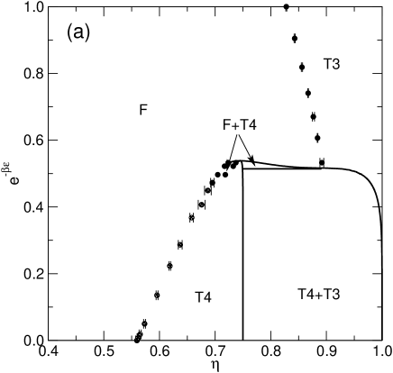
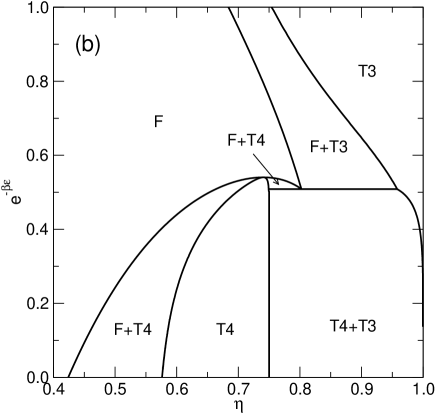
Figure 2: Temperature-density phase diagram from Monte Carlo simulations (a) and LFMT (b). The three phases are labeled F for the fluid, and T3 and T4 for the two solids. Coexistence regions are marked with two labels.

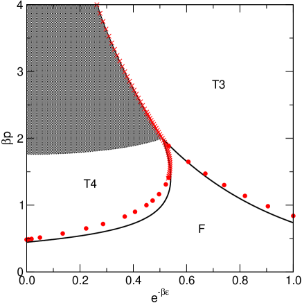
Figure 3: Pressure-temperature phase diagram. The vertical axis represents the pressure divided by $k_{B}T$ ($\beta p$) and the horizontal axis represents the temperature in the form $e^{-\beta\epsilon}$, with $\epsilon>0$ the soft repulsion between NNN sites. Symbols are the Monte Carlo simulations and lines represent the predictions of the LFMT. The shaded region is a set of values that cannot be reached because the pressure jumps discontinuously at the T3–T4 transition.

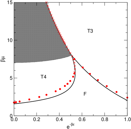
Figure 4: Same as Fig. 3 but for the chemical potential $\mu$. The shaded region is a set of values that cannot be reached because the chemical potential jumps discontinuously at the T3–T4 transition.

The results for the F–T3 transition are collected in Table 1 (notice that the densities are expressed in terms of packing fractions, i.e. $\eta=3\langle N\rangle/M$), and plotted in Figs. 2, 3, and 4. The particular case $\beta\epsilon=0$ corresponds to the so-called hard hexagon model, whose critical properties are known exactly.JPAMG_1980_13_L61 ; baxter2 The exact values are $\beta\mu_{c}=\log\left[(11+5\sqrt{5})/2\right]\approx 2.4061$, and $\eta_{c}=3\rho_{c}=3(5-\sqrt{5})/10\approx 0.8292$. A comparison with the extrapolations given in Table 1 suggests that the latter are quite accurate —though not perfect— in the estimation of the exact values.

The results for $\eta_{c}(\beta\epsilon)$ and $\beta\mu_{c}(\beta\epsilon)$ are well represented by the fits

$$\eta_{\rm F-T3}(\beta\epsilon) = 0.8280+0.1582\beta\epsilon-0.0922(\beta\epsilon)^{2},$$ (44)

$$\beta\mu_{\rm F-T3}(\beta\epsilon) = 2.4056+7.3074\beta\epsilon+1.6079(\beta\epsilon)^{2}$$ (45)

$$-0.5478(\beta\epsilon)^{3}.$$

VI.1.2 F–T4 transition

As in the previous case, we have selected a number of representative temperatures and performed simulations for several system sizes. In most cases we considered the same sizes ($L$=12, 18, $\cdots$, 60) as for the F–T3 transition. In addition to $\beta\mu_{c}(L,T)$ and $\rho_{c}(L,T)$ we also payed attention to the quantities $m_{2}(L,T)$ and $g_{4}(L,T)$ because this transition appears to be discontinuous in some cases.

The precise location of the multi-critical point —where the transition changes from continuous to discontinuous— is a hard task due to the first order transition being quite weak. In order to make an approximate estimation we focused on the changes of $g_{4}(L,T)$ with $L$ and found that the change of character of the transition occurs at about $\beta\epsilon\approx 0.75\pm 0.05$. Surprisingly, it is precisely at this temperature that the simulation results are well represented by the scaling law (19).

For $\beta\epsilon>0.75$ we have estimated the critical properties of the F–T4 line in the thermodynamic limit using the same strategy as for the F–T3 case, employing the critical exponents of the 4-state Potts model in two dimensions. The results are gathered in Table 2. The results at low temperature show a good agreement with those reported by Zhang and Deng PRE_2008_78_031103 : $\beta\mu_{c}=1.75682(2)$, and $\eta_{c}=0.540(12)$.

$\beta\epsilon$	$\beta\mu_{c}$	$\eta_{c}$
1000	1.756(1)	0.560(2)
10	1.756(2)	0.560(2)
5	1.774(1)	0.562(2)
4	1.806(1)	0.565(2)
3	1.897(1)	0.573(2)
2	2.165(1)	0.596(2)
1.5	2.491(2)	0.619(2)
1.25	2.777(3)	0.637(4)
1.0	3.246(4)	0.658(4)
0.9	3.541(3)	0.676(5)
0.8	3.950(2)	0.688(4)
0.75	4.230(2)	0.695(3)

Table 2: Computed points for the continuous F–T4 transition. Error bars are given in brackets, in units of the last figure of the property, and correspond to a confidence level of about 95%.

For $\beta\epsilon<0.75$ the plot of the chemical potential as a function of $\eta$ shows a loop for the different system sizes considered. This is a signature of a first order phase transition. The change in density is quite small, and the transition is rather weak. Taking this into account we have estimated the location of the transitions by fitting the results for each simulated temperature to equations of the form (43), with $b_{x}=1$, $m=2$. The properties considered were $\mu_{c}(L,T)$, $\eta_{c}(L,T)$, and $\Delta\eta_{c}(L,T)=\sqrt{m_{2}(L,T)}$. Notice that, in general, for discontinuous transitions $\lim_{L\rightarrow\infty}m_{2}(L,T)\neq 0$. Thus, in the thermodynamic limit, the packing fractions of the two coexisting phases are then obtained as

$$\eta_{F}(T) = \eta_{c}(T)-\Delta\eta_{c}(T)$$ (46)

$$\eta_{T4}(T) = \eta_{c}(T)+\Delta\eta_{c}(T)$$ (47)

The results for the discontinuous F-T4 transition are collected in Table 3.

$\beta\epsilon$	0.70	0.65	0.63
$\beta\mu_{F-T4}$	4.61(2)	5.18(2)	5.59(4)
$\eta_{F}$	0.705(2)	0.717(2)	0.724(2)
$\eta_{T4}$	0.718(2)	0.733(2)	0.737(2)

Table 3: Computed points for the discontinuous F-T4 transition. Error bars are given between parentheses, in units of the last figure of the property and correspond to a confidence level of about 95 %

VI.2 Gibbs-Duhem Integration

After a number of tests we analyzed the discontinuous T3–T4 transitions and its continuation as F–T4 transition using GDI with lattices of size $L=120$. This relatively large size was chosen since the end of this line at low values of $\beta\mu$ corresponds to the equilibrium between a low density fluid and the T4 phase. This transition is relatively weak and because of this we found that for smaller values of $L$ one of the subsystems often undergoes a phase transition and both subsystems end up in the same phase, with the corresponding breakdown of the GDI scheme. The use of large simulation boxes then makes possible us to reach values of $\beta\mu$ that allowed us to check the consistency between GDI and WL simulations. Technical details of the integration algorithm can be found elsewhere.hoye ; Lomba et al. (2007) The integration steps and length of the simulations were chosen after performing a number of tests.

The GDI was divided in two parts. In the first part we perform an integration following the scheme given in Eq. (14). The first point was chosen to be $T^{*}=(\beta\epsilon)^{-1}=0.35$, $\mu/\epsilon=12$. The integration was carried out using a temperature step of $\Delta T^{*}=0.025$. At each step we run long simulations ($2\times 10^{6}$ cycles, each cycle including $M/3$ insertion/deletion attempts; averages are taken over the second half of the simulation). The integration was carried out up to $T^{*}=1.25$ (or $\beta\epsilon=0.80$), where we get coexistence for $\mu/\epsilon=11.947\pm 0.001$.

The second part of the integration was carried out using the scheme given in Eq. (15). The starting point was that defined by the previous integration ($T^{*}=1.25$, $\beta\epsilon=0.80$, $\beta\mu=9.558$). The integration step was then $\Delta(\beta\mu)=-0.020$, and the length of the simulations was about $1\times 10^{6}$ cycles (for each system and step, averaging over the second half of each run). As in the previous part, a number of additional simulations with larger integration steps, smaller system sizes, and shorter runs, were carried out in order to test the integration accuracy and to estimate error bars.

Simulations were launched to execute 201 integration steps (to reach, in principle, a final value of $\beta\mu=5.558$). We observed that for this line GDI required both large systems and precise estimates of the integrand in order to avoid the collapse of the method before reaching the F–T4 discontinuous equilibrium found with WL simulations. For instance, using large simulations (precise integrands) with $L=60$, $\Delta(\beta\mu)=-0.05$, it was possible to get good estimates both for the triple point T4–F–T3 and for the temperature at which the density of phases F and T3 are equal at equilibrium, but shortly after reaching the latter point the algorithm failed due to the transition of one of the phases into the other. With $L=120$ the integration stayed stable until reaching the expected final value of $\beta\mu\simeq 5.56$, which was found to be consistent, within statistical uncertainty, with the value of the F–T4 equilibrium obtained through WL simulation at $\beta\epsilon=0.63$.

From the results obtained with GDI, together with those previously reported on the F–T3 transition, we can estimate the position of two of the special points in the phase diagram, namely the triple point T4–F–T3 and the point of maximum temperature for the F–T4 equilibrium (at this point both phases have the same density). These results, together with those of the change of the transition order of the F–T4 equilibrium, are collected in Table 4.

Point	TP (T4-F-T3)	HT (F-T4)	DC (F-T4)
$\beta\epsilon$	0.660(2)0	0.619(1)	$\sim$ 0.750
$\beta\mu$	7.78(2)00	6.35(2)0	$\sim$ 4.00
$\eta_{F}$	0.892(5)0	0.745(1)	$\sim$ 0.69
$\eta_{T3}$	0.892(5)0	—	—
$\eta_{T4}$	0.7491(1)	0.745(1)	$\sim$ 0.69

Table 4: Singular points of the phase diagram: TP stands for triple point, HT for high temperature end-point, and DC for the change from discontinuous to continuous behavior of the fluid-T4 transition. Error bars are estimated by comparing results from different GDI trajectories.

VI.3 LFMT calculations

We shall now apply the density functional obtained in Sec. V to determine the temperature-density phase diagram of this fluid. To this purpose we have to study the three phases involved: the uniform fluid and the two solid lattices (T3 and T4, c.f. Fig. 1).

VI.3.1 Uniform fluid

If every site has the same average occupancy $\rho$ (hence a packing fraction $\eta=3\rho$), the free energy per unit volume (in $k_{B}T$ units) will be

$$\begin{split}\Phi=&\,\rho\ln\rho+(1-\rho)\ln(1-\rho)-4(1-3\rho)\ln(1-3\rho)\\ &+3(1-4\rho)\ln(1-4\rho+\rho_{14})+6\rho\ln\left(1-\frac{\rho_{14}}{\rho}\right),\end{split}$$ (48)

where $\rho_{14}=\rho_{14}(\rho,\rho,\rho,\rho)$ is

$$\begin{split}\rho_{14}=&\,\frac{1}{2(1-\kappa)}\Big{\{}2(2-\kappa)\rho-1\\ &\left.+\sqrt{1-4(2-\kappa)\rho+4(4-3\kappa)\rho^{2}}\right\}.\end{split}$$ (49)

The pressure can then be obtained as

$$\beta p=\rho^{2}\frac{\partial(\Phi/\rho)}{\partial\rho}=\ln\left[\frac{(1-3\rho)^{4}}{(1-4\rho+\rho_{14})^{3}(1-\rho)}\right],$$ (50)

and the chemical potential is given by $\beta\mu=(\Phi+\beta p)/\rho$.

VI.3.2 T3 solid phase

The T3 solid occupies one of the three sublattice shown in Fig. 1(a). From this figure it is clear that the density profile will take one out of two values: The sites of the occupied sublattice —marked with large circles in Fig. 1(a)— will have a higher density $\rho_{A}$, whereas the remaining ones will have a lower density $\rho_{B}$ (by symmetry this value is the same for all those sites). The packing fraction will then be $\eta=\rho_{A}+2\rho_{B}$.

If we regard the lattice as a tiling of rhombii, we can realize that there are three different kinds of them: Those with $\rho_{A}$ at positions $1$ and $4$ and $\rho_{B}$ at positions $2$ and $3$, those with $\rho_{A}$ only at position $2$, and those with $\rho_{A}$ only at position $3$. There is the same number of each kind. The contribution of the two latter to the rhombic cavities will be the same, but different from the contribution of the former. Thus

$$\sum_{C\in\mathcal{W}_{4}}\frac{\Phi_{0}(C)}{V}=\Phi_{0}(\rho_{A},\rho_{B},\rho_{B},\rho_{A})+2\Phi_{0}(\rho_{B},\rho_{A},\rho_{B},\rho_{B}),$$ (51)

with $\Phi_{0}(\bm{\rho})$ given by (41). As for the triangular cavities, $\sum_{i}\rho_{i}=\rho_{A}+2\rho_{B}=\eta$ for any of them, so

$$\sum_{C\in\mathcal{W}_{3}}\frac{\Phi_{0}(C)}{V}=2\eta+2(1-\eta)\ln(1-\eta).$$ (52)

Dimers do not contribute to the functional, so the last contribution will be

$$\begin{split}\sum_{C\in\mathcal{W}_{1}}\frac{\Phi_{0}(C)}{V}=&\,\frac{\eta}{3}+\frac{1}{3}(1-\rho_{A})\ln(1-\rho_{A})\\ &+\frac{2}{3}(1-\rho_{B})\ln(1-\rho_{B}).\end{split}$$ (53)

Putting all together and adding the ideal part the result is

$$\begin{split}\Phi(\rho_{B};\eta)=&\,\frac{1}{3}(1-\eta+2\rho_{B})\ln(1-\eta+2\rho_{B})+\frac{2}{3}(1-\rho_{B})\ln(1-\rho_{B})-4(1-\eta)\ln(1-\eta)\\ &+(1-2\eta+2\rho_{B})\ln(1-2\eta+2\rho_{B}+\xi_{1})+2(1-\eta-\rho_{B})\ln(1-\eta-\rho_{B}+\xi_{2})\\ &+(\eta-2\rho_{B})\left\{2\ln(\eta-2\rho_{B}-\xi_{1})-\frac{5}{3}\ln(\eta-2\rho_{B})\right\}+2\rho_{B}\left\{2\ln(\rho_{B}-\xi_{2})-\frac{5}{3}\ln\rho_{B}\right\},\end{split}$$ (54)

where we have eliminated $\rho_{A}=\eta-2\rho_{B}$, and

$$\xi_{1} = \rho_{14}(\rho_{A},\rho_{B},\rho_{B},\rho_{A}),$$ (55)

$$\xi_{2} = \rho_{14}(\rho_{B},\rho_{A},\rho_{B},\rho_{B}).$$ (56)

The free energy as a function of $\eta$ is obtained by minimizing the function (54) with respect to $\rho_{B}$ (always taking the solution $\rho_{B}\leq\eta/3$). For $\kappa>\kappa_{t}=0.5086\dots$ (see below) there is a first order transition from a homogeneous fluid to the T3 solid [see Fig. 2]. In the limit $\kappa=1$ where the model becomes identical to the hard hexagon model, we find a wide first order transition. This model has been previously solved within the LFMT approach in Ref. lafuente:2003b, . LFMT is a mean-field-like theory, and therefore all second order transitions have a parabolic behavior of the order parameter —corresponding to a critical exponent $\beta=1/2$. The exponent of the hard hexagon model (like that of the 3-state Potts model) isJPAMG_1980_13_L61 ; baxter2 $\beta=1/9$. Looking at Figure 7 of Ref. lafuente:2003b, one must admit that a discontinuous function is a better approximation to the behavior of the order parameter than a parabolic, mean-field one. So although not quite satisfying, the result is quantitatively not too inaccurate. This also reflects in the fact that the pressure and chemical potential at the transition is rather close to the exact value, and it remains so for all $\kappa_{t}<\kappa<1$, as Figs. 3 and 4 show.

VI.3.3 T4 solid phase

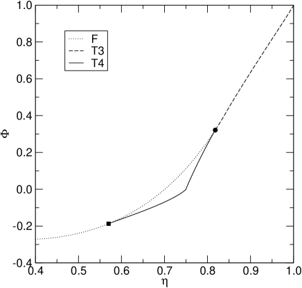
Figure 5: Free energy (in $k_{B}T$ units) per unit volume as a function of the packing fraction $\eta$, for $\kappa=e^{-\beta\epsilon}=0.3679$, below the triple point. Dotted line represents the free energy of the uniform fluid; solid line that of the T4 phase, and dashed line that of the T3 phase. The filled square represents the bifurcation point F–T3, and the filled circle the bifurcation point T3–T4. Notice the discontinuity of the derivative of the free energy at $\eta=0.75$, the close packing of the NNN exclusion lattice gas. For $\eta>0.75$ the free energy of the T4 phase is concave, so T4–T3 coexistence always occurs with a T4 phase at $\eta=0.75$, and both the chemical potential and the pressure jump discontinuously at this transition.

The T4 solid occupies one of the four sublattice shown in Fig. 1(b). Again the density profile will take either the value $\rho_{A}$ at the sites of the occupied sublattice —marked with large circles in Fig. 1(b)— or the value $\rho_{B}$ at the remaining sites (the same for all of them, by symmetry). The packing fraction will now be $\eta=\rho_{A}+3\rho_{B}$.

As a tiling of rhombii the lattice contains four kinds of them, each with an A site at one of the four positions. There is the same amount of each type. Thus

$$\begin{split}\sum_{C\in\mathcal{W}_{4}}\frac{\Phi_{0}(C)}{V}=&\,\frac{3}{2}\Phi_{0}(\rho_{A},\rho_{B},\rho_{B},\rho_{B})\\ &+\frac{3}{2}\Phi_{0}(\rho_{B},\rho_{A},\rho_{B},\rho_{B}).\end{split}$$ (57)

As for the triangles, one fourth of them have an A site and two B sites, and three fourths have three B sites, so

$$\begin{split}\sum_{C\in\mathcal{W}_{3}}\frac{\Phi_{0}(C)}{V}=&\,\frac{\rho_{A}+2\rho_{B}}{2}+\frac{1}{2}(1-\rho_{A}-2\rho_{B})\\ &\times\ln(1-\rho_{A}-2\rho_{B})+\frac{3}{2}\rho_{B}\\ &+\frac{3}{2}(1-3\rho_{B})\ln(1-3\rho_{B}).\end{split}$$ (58)

Finally, the contribution of the point-like cavities (those of $\mathcal{W}_{1}$) is

$$\begin{split}\sum_{C\in\mathcal{W}_{1}}\frac{\Phi_{0}(C)}{V}=&\,\frac{\eta}{4}+\frac{1}{4}(1-\rho_{A})\ln(1-\rho_{A})\\ &+\frac{3}{4}(1-\rho_{B})\ln(1-\rho_{B}),\end{split}$$ (59)

because $1/4$ of the sites are of type A and $3/4$ of type B.

Putting all together and adding the ideal part the result is

$$\begin{split}\Phi(\rho_{B};\eta)&=\frac{3-4\eta}{2}\left\{\ln\left(1-\frac{4\eta}{3}+\lambda_{1}\right)+\ln\left(1-\frac{4\eta}{3}+\lambda_{2}\right)\right\}+\frac{4\eta-9\rho_{B}}{2}\ln\left(\frac{4\eta}{3}-3\rho_{B}-\lambda_{1}\right)\\ &+\frac{3\rho_{B}}{2}\{\ln(\rho_{B}-\lambda_{1})+2\ln(\rho_{B}-\lambda_{2})\}+\frac{3}{4}(1-\rho_{B})\ln(1-\rho_{B})-(1-3\rho_{B})\ln(1-3\rho_{B})\\ &-\frac{15}{4}\rho_{B}\ln\rho_{B}-3\left(1-\frac{4\eta}{3}+\rho_{B}\right)\ln\left(1-\frac{4\eta}{3}+\rho_{B}\right)+\frac{1}{4}\left(1-\frac{4\eta}{3}+3\rho_{B}\right)\ln\left(1-\frac{4\eta}{3}+3\rho_{B}\right)\\ &-\frac{5}{4}\left(\frac{4\eta}{3}-3\rho_{B}\right)\ln\left(\frac{4\eta}{3}-3\rho_{B}\right),\end{split}$$ (60)

where we have eliminated $\rho_{A}=\eta-3\rho_{B}$, and

$$\lambda_{1} = \rho_{14}(\rho_{A},\rho_{B},\rho_{B},\rho_{B}),$$ (61)

$$\lambda_{2} = \rho_{14}(\rho_{B},\rho_{A},\rho_{B},\rho_{B}).$$ (62)

As for T3, the free energy of the equilibrium phase is obtained by minimization of this function with respect to $\rho_{B}$ (always choosing the solution $\rho_{B}\leq\eta/4$). In the limit $\kappa=0$ the model is equivalent to a lattice gas with NNN exclusion. In this limit we obtain a wide first order transition from a uniform fluid to a T4 solid, which again is found to be continuous in the simulations. The values of the pressure and chemical potential for this transition are nevertheless rather accurately predicted (see Figs. 3 and 4), so the same considerations as for the F–T3 transition in the hard hexagon ($\kappa=1$) limit hold here. We find a first-order F–T4 transition all the way up to $\kappa_{c}=0.5403\dots$, where it coalesces to an end-point (at $\eta_{c}=0.7405\dots$). It is to be noticed that this point is obtained with high accuracy (simulations yield $\kappa_{c}\approx 0.538$ and $\eta_{c}\approx 0.745$; see Table 4), and that simulations also find a first-order F–T4 transition near this point (see Fig. 2).

When $\kappa=0$ the model has a close-packing at $\eta=3/4$; however, for any $\kappa>0$ this limit can be crossed, although at a very high energetic cost. Once this cost is paid, the system greatly diminishes its entropy by reordering itself in a T3 structure. Hence the transition that is found, for all $\kappa$ up to not too far from $\kappa_{t}$, between a close-packed T4 solid and a nearly closed-packed T3 solid, which is also observed in the simulations (see Fig. 2). What happens with the free energy at this T4–T3 transition is very peculiar and it is illustrated in Fig. 5. The derivative of the free energy per unit volume (in $k_{B}T$ units) with respect to the packing fraction is discontinuous at $\eta=3/4$. The free energy of the T4 phase is concave beyond this point, so there is a T4–T3 coexistence, but it does not satisfy the standard conditions of phase equilibria. As a matter of fact, both the pressure and the chemical potential jump discontinuously at this point. This creates a “forbidden” region in the pressure-temperature and the chemical potential-temperature, which can be observed in Figs. 3 and 4.

At the value $\kappa_{t}$ there is a F–T3–T4 triple point, which the theory predicts very close to the value obtained in the simulations, $\kappa_{t}\approx 0.517$ (see Table 4).

In the range $\kappa_{t}<\kappa<\kappa_{c}$ a reentrant T4–F transition is found before the F–T3 transition occurs. This reentrant behavior also appears in the simulations, although the coexistence region is wider because the F–T3 transition is continuous (see Fig. 2).

VII Discussion

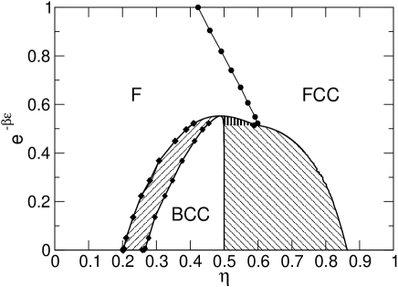
Figure 6: Temperature-density phase diagram for the 3d counterpart of the model discussed in this article, on a simple cubic lattice.

From Figs. 2, 3, and 4, we see that the theoretical results for the equilibrium between the ordered phases are in reasonably good agreement with the simulation. The theoretical estimations of the triple point and the high temperature end-point of the F–T4 equilibrium are also well described. On the other hand the LFMT description of the order-disorder transitions, both at low and high temperature is less accurate. The theory predicts first order transitions whereas they are continuous in both limits. We have argued that this is so because the behavior of the order parameter is very sharp (the critical exponent $\beta=1/9$), so much that a discontinuous function is a better approximation to it than the simple parabolic behavior predicted by any mean-field-like theory (like this one). The theory can in principle be refined by considering larger “maximal cavities”. Although it would produce a far more complicated theory than the one presented here, and it is expected that its accuracy would increase, it is doubtful that the order of the transition would be corrected. No matter how much we complicate the theory, it does not cure its mean-field behavior near the transitions. This is also the reason why first-order transitions are described much better.

In favor of this argument is the fact that, overall, the agreement between simulation and theoretical transition lines in the planes $\beta\mu$–$T$ and $\beta p$–$T$ is rather good.

When comparing the phase diagram for the two-dimensional system on the triangular lattice with that of the three-dimensional systemhoye [c.f. Fig. 6] in a simple cubic lattice we find a couple of qualitative differences. The first one concerns the nature of the order-disorder transition at low temperature, which is continuous in two dimensions and discontinuous in three dimensions. This difference can be understood in terms of the different dimensionality, and can be related with the critical behavior of Potts models RMP_1982_54_235 in two and three dimensions.

The second relevant difference arises when comparing the transitions between the two ordered phases. In two dimensions, at solid-solid equilibrium the high density solid is nearly close packed for a wide range of temperatures, whereas this is not the case for its three dimensional counterpart even at the lowest temperatures. This difference can be explained as follows. At low temperature phase equilibrium is essentially controlled by the condition of minimum energy. The energy per unit volume of the closed packed configuration in two dimensions is $\bar{u}^{*}=\mathcal{U}/M\epsilon=3$. At slighly lower $\eta$ there are vacancies. The way in which they minimize the energy is by not being nearest neighbors in the solid lattice (i.e. next-nearest neighbors in the underlying lattice). This way each vacancy reduces the energy by $6\epsilon$. Thus, for $2/3<\eta\leq 1$, $\bar{u}^{*}(\eta)=2\eta-1$. If we consider, at the same density, a system separated into a close-packed T3 and a T4 phase, then $N_{\rm T3}+N_{\rm T4}=N$ and $3N_{\rm T3}+4N_{\rm T4}=M$, and the energy of this system will be $U=3\epsilon N_{\rm T3}$. Hence $\bar{u}^{*}(\eta)=4\eta-3$. Since $4\eta-3<2\eta-1$ for all $\eta<1$, then the phase separated system is energetically favored. The same argument for the three-dimensional model of Høye et al. hoye yields the same energy, $\bar{u}^{*}(\eta)=6\eta-3$ (for $3/4\leq\eta\leq 1)$ in both cases, so in the three dimensional system the entropy does play a role in defining the density of the high density solid, and the number of vacancies does not go to zero when approaching $T=0$.

The similarity between the phase diagrams in two and three dimensions is remarkable, though. Peculiar features like the reentrant fluid phase or the vertical line at the closest packing of the loose solid when it coexists with the dense one, appear in both cases.

Much to our surprise, we have realized that the LFMT for the three-dimensional model is far more complicated than that of the two-dimensional one. The reason is that the soft repulsion at NNN allows for maximal cavities with up to four particles at the same time. This not only introduces a much larger set of cavities to elaborate the density functional, but also the corresponding expressions for the $\Phi_{0}$ functions is very cumbersome and hard to handle. On the other hand, given the similarity between the phase diagrams, it seems that the physics of the model is already well captured by the two-dimensional version.