Self-sustained current oscillations in the kinetic theory of semiconductor superlattices

Abstract

We present the first numerical solutions of a kinetic theory description of self-sustained current oscillations in n-doped semiconductor superlattices. The governing equation is a single-miniband Boltzmann-Poisson transport equation with a BGK (Bhatnagar-Gross-Krook) collision term. Appropriate boundary conditions for the distribution function describe electron injection in the contact regions. These conditions seamlessly become Ohm’s law at the injecting contact and the zero charge boundary condition at the receiving contact when integrated over the wave vector. The time-dependent model is numerically solved for the distribution function by using the deterministic Weighted Particle Method. Numerical simulations are used to ascertain the convergence of the method. The numerical results confirm the validity of the Chapman-Enskog perturbation method used previously to derive generalized drift-diffusion equations for high electric fields because they agree very well with numerical solutions thereof.

1 Introduction

When non-interacting electrons in the conduction band of a material are subject to a constant electric field $E$, their positions should oscillate with a frequency proportional to the electric field, $\omega_{B}=eEl/\hbar$, where $-e<0$, $\hbar$ and $l$ are the charge of the electron, the Planck constant and the crystal period. These coherent Bloch oscillations (BO) and the associated current were predicted by Zener in 1934 [21]. Scattering limits the observability of BO: to observe them, their period should be smaller than the scattering time $\tau$, so that $E>\hbar/(el\tau)$. In standard materials, the fields required to observe BO are too large and therefore damped Bloch oscillations were not found until 1992 in experiments with undoped semiconductor superlattices [11], which have much larger periods than natural crystals.

Semiconductor superlattices are artificial one-dimensional crystals formed by epitaxial growth of layers belonging to two different semiconductors that have similar lattice constants [4]. They were synthesized following Esaki and Tsu’s idea that these artificial crystals would be useful to realize BO or related high frequency oscillations [8]. The difference in the energy gaps of the component semiconductors makes the conduction band of the superlattice to be a periodic succession of barriers and wells with typical periods of several nanometers. The electronic spectrum of a superlattice (SL) consists of a succession of minibands and minigaps generated by its periodicity. Tayloring the size of barriers and wells and the negative doping density of the latter, it is possible to achieve SLs with wide minibands and to populate only the lowest one. Electrons moving in this miniband have energies that are periodic functions of their wave numbers and are scattered by phonons, impurities and other electrons. When an appropriate dc voltage is held between the ends of one such SL with finitely many periods, it is possible to obtain high-frequency self-sustained oscillations of the current through the structure [4]. These oscillations are caused by repeated formation of electric field pulses at the injecting contact of the SL that move forward and disappear at the receiving contact. Thus they are transit-time oscillations whose frequency is inversely proportional to the SL length: they are similar to the Gunn effect in bulk semiconductors [18] and are different from BO. These Gunn-type oscillations have been observed in experiments with GaAs/AlAs SL (and with other SL based on III-V semiconductors) since 1996 and are the basis of fast oscillator devices [13]. The connection between the existence of Gunn-type oscillations and the suppression of Bloch oscillations is not yet well understood despite theoretical and experimental efforts [4].

Although mathematical models at the level of semiclassical kinetic theory go back to the 1970s [19], their analysis has been based on simplified reduced ordinary differential equations [14, 15] which typically ignore space charge effects. Electron transport in a single miniband SL can be described by a kinetic equation coupled to a Poisson equation approximately describing the electric potential due to the other electrons [3]. A simple kinetic equation [14] contains an energy-dissipating collision term of Bhatnagar-Gross-Krook (BGK) type [1] and a simple energy-conserving (but momentum-dissipating) collision term. This model does not include coupling to the Poisson equation. An important point is that the dispersion relation between miniband energy and momentum is periodic because this periodicity gives rise to a relation between electron drift velocity and electric field which has a maximum value [4]. Then the drift velocity decreases as the field increases for large field values (negative differential mobility) and this in turn causes the Gunn-type self-sustained current oscillations (SSCO) for appropriate bias and contact boundary conditions [4]. These features are absent in the more usual Boltzmann-Poisson systems with parabolic band dispersion relations.

Recently, Bonilla et al [3] have derived a nonlinear drift-diffusion equation from the KSS-BGK kinetic model coupled to the Poisson equation, which we will call the BGK-Poisson system. They use a Chapman-Enskog perturbation method in a particular limit in which the collision terms are of the same order as the term containing the electric field and dominate all other terms in the kinetic equation. Then stable SSCO are obtained by numerically solving the drift-diffusion equation with appropriate boundary and initial conditions [3]. However, no one has solved numerically the kinetic equation directly and shown that self-oscillations are among its solutions or studied the relation between these solutions and those of the limiting drift-diffusion equation. These are the problems tackled in the present paper and solving them could be a step in more precise studies of stable current oscillations in superlattices and other low dimensional solid state systems.

We solve the BGK-Poisson kinetic equation model by means of a deterministic weighted particle method that has been used in the past to solve Boltzmann equations with non-periodic energy band dispersion relations [20]. Particle methods (see a recent one in [10]) are appropriate to study our system of equations because their solutions may present large gradients: the electric field pulses obtained by simulating the approximate drift-diffusion equations have a smooth leading front but a steep trailing back front [4]. The present work paves the way to numerically solving interesting problems in nanoelectronics and spintronics that are described by related quantum kinetic equations with more than one miniband [2].

2 The Model

Our model for electron transport in a single miniband SL is a Boltzmann-Poisson system with BGK collision term [1] plus appropriate boundary and initial conditions. The governing equations are:

$$\partial_{t}f+v(k)\partial_{x}f+\frac{eF}{\hbar}\partial_{k}f=-\nu_{en}\left(f-f^{FD}\right)-\frac{\nu_{imp}}{2}[f-f(x,-k,t)],$$ (1)

$$\epsilon\partial_{x}^{2}V=\frac{e}{l}\left(n-N_{D}\right),\quad F=\partial_{x}V,$$ (2)

$$n=\frac{l}{2\pi}\int_{-\frac{\pi}{l}}^{\frac{\pi}{l}}f(x,k,t)\,dk=\frac{l}{2\pi}\int_{-\frac{\pi}{l}}^{\frac{\pi}{l}}f^{FD}(k;\mu(n))\,dk,$$ (3)

$$f^{FD}(k;\mu)=\frac{m^{*}k_{B}T}{\pi\hbar^{2}}\ln\left[1+\exp\left(\frac{\mu-\varepsilon(k)}{k_{B}T}\right)\right],$$ (4)

with $x\in[0,L]$ and $f$ periodic in $k$ with period $2\pi/l$. Here $l$, $L=Nl$, $N$, $\epsilon$, $f$, $n$, $N_{D}$, $k_{B}$, $T$, $V$, $-F$, $m^{*}$ and $-e<0$ are the SL period, the SL length, the number of SL periods, the dielectric constant, the one-particle distribution function, the 2D electron density, the 2D doping density, the Boltzmann constant, the lattice temperature, the electric potential, the electric field, the effective mass of the electron, and the electron charge, respectively. We shall describe boundary and initial conditions later.

The first term in the right hand side of Eq. (1) represents energy relaxation towards a 1D effective Fermi-Dirac distribution $f^{FD}(k;\mu(n))$ [3] (local equilibrium) due to e.g. phonon scattering. $\nu_{en}$ is the collision frequency, taken as constant for simplicity. Here, $\mu(n)$ is the chemical potential that is a function of $n$ resulting from solving equation (3) when (4) is substituted in it. A similar BGK model with a Boltzmann local distribution function was proposed by Ignatov and Shashkin [14, 15]. The second term in the right hand side of Eq. (1) accounts for impurity elastic collisions with the constant collision frequency $\nu_{imp}$, which conserve energy but dissipate momentum [19, 3, 4]. Transfer of lateral momentum due to impurity scattering [12] is ignored in this model. We assume the simple tight-binding miniband dispersion relation,

$$\varepsilon(k)=\frac{\Delta}{2}\left(1-\cos kl\right)\Longrightarrow v(k)=\frac{1}{\hbar}\,\frac{d\varepsilon}{dk}=\frac{l\Delta}{2\hbar}\,\sin kl,$$ (5)

where $\Delta$ is the miniband width. The exact and Fermi-Dirac distribution functions, $f$ and $f^{FD}$, have the same electron density $n$, according to (3). The latter equation is solved for the chemical potential $\mu$ in terms of $n$, which yields the function $\mu(n)$. When (1) is integrated over $k$, we obtain the charge continuity equation,

$$\partial_{t}n+\frac{l}{e}\partial_{x}J_{n}=0,\quad\mbox{with}$$ (6)

$$J_{n}=\frac{e}{2\pi}\int_{-\pi/l}^{\pi/l}v(k)\,f(x,k,t)\,dk,$$ (7)

where $J_{n}$ is the electron current density.

2.1 Voltage bias condition

Using the Poisson equation (2) to eliminate $n$, we obtain the following form of Ampère’s law:

$$\epsilon\,\partial_{t}F+J_{n}=J(t),$$ (8)

where $J(t)$ is the total current density. The total current density can be obtained from the voltage bias condition:

$$\Phi(t)\equiv\frac{1}{L}\int_{0}^{L}F(x,t)\,dx=\phi,$$ (9)

where $\Phi(t)L$ is the voltage between the two contacts at the end of the SL and $\Phi(t)$ is an average field. For dc voltage bias, $\Phi(t)$ is a fixed constant $\phi$. If we integrate (8) over $x$ and use (9), we obtain

$$J(t)=\frac{1}{L}\int_{0}^{L}J_{n}(x,t)\,dx.$$ (10)

2.2 Boundary conditions

The boundary conditions give the distribution function $f$ on the contacts at $x=0$ and $x=L$ through the distribution function inside the semiconductor. For fixed $|k|$, there are two possible characteristic curves at a point $(x,t)$: one for $k>0$ and another one for $k<0$. With $k<0$ the characteristic curve for $x\to 0+$ and $t>0$ is given by the initial condition whereas it is given by the distribution function at the contact ($x=0$) if $k>0$. Then, for $x=0$ we need to specify the distribution function at the contact for $k>0$, $f^{+}$, whereas for $x=L$ we need to specify the distribution function at the contact for $k<0$, $f^{-}$. Instead of inventing a theory for injecting and collecting contacts, we use a top-down approach proposed in Ref. [4]: we know that the following boundary conditions appropriately describe current self-oscillations in the drift-diffusion equation for the electric field,

$$J_{n}(0,t)=\sigma\,F(0,t),$$ (11)

$$n(L,t)=N_{D},$$ (12)

where $\sigma>0$ is the constant contact conductivity and the left hand side of Eq. (11) is the electron current density. We will use boundary conditions for $f$ such that they become (11) and (12) when we integrate them according to the definitions (3) and (7) of $n$ and $J_{n}$ respectively:

$$f^{+}=\frac{2\pi\hbar\sigma F}{e\Delta}-\frac{f^{(0)}}{\int_{0}^{\frac{\pi}{l}}v(k)f^{(0)}\,dk}\int_{-\frac{\pi}{l}}^{0}v(k)f^{-}\,dk,$$ (13)

for $x=0$, and

$$f^{-}=\frac{f^{(0)}}{(l/2\pi)\int_{-\frac{\pi}{l}}^{0}f^{(0)}\,dk}\left(N_{D}-\frac{l}{2\pi}\int_{0}^{\frac{\pi}{l}}f^{+}\,dk\right),$$ (14)

for $x=L$. Note that the integral over $k$ of (13) times $e\,v(k)/(2\pi)$ yields (11) and the integral over $k$ of (14) times $l/(2\pi)$ yields (12). In these equations, $f^{(0)}$ is the leading order approximation for the distribution function in the Chapman-Enskog method [3, 4]:

$$f^{(0)}(k;n,F)=\sum_{j=-\infty}^{\infty}f_{j}^{(0)}\exp\left(\imath jkl\right),$$ (15)

where

$$f_{j}^{(0)}=\frac{1-\imath j\varphi/\tau_{e}}{1+j^{2}\varphi^{2}}f_{j}^{FD}$$

$$f_{j}^{FD}=\frac{l}{\pi}\int_{0}^{\frac{\pi}{l}}f^{FD}\cos(jkl)\,dk$$

$$\varphi=\frac{F}{F_{M}}\qquad F_{M}=\frac{\hbar\sqrt{\nu_{en}(\nu_{en}+\nu_{imp})}}{el}\qquad\tau_{e}=\sqrt{1+\frac{\nu_{imp}}{\nu_{en}}}.$$

Eq. (15) is the solution of (1) when we drop the $x$ and $t$ derivatives of $f$ (see [3]).

If we use the electric potential $V$ instead of the field $F=\partial V/\partial x$ (recall that the true electric field is $-F$), the following boundary conditions for $V$ are compatible with (9):

$$V(0,t)=0,\quad V(L,t)=\phi L=\int_{0}^{L}F(x,t)\,dx.$$ (16)

2.3 Initial condition

We select (15) as our initial condition for the distribution function. The initial electric field is assumed to be constant, $F(x,0)=\phi$, where $\phi$ is the average field. If we start from other initial conditions, the evolution of the current and other magnitudes are similar to those presented here after about 0.3 ps.

Recapitulating, the equations governing our model are (1) - (4) for the unknowns $f$ and $V$ with initial condition (15) and boundary conditions (13), (14) and (16). If we use the field $F$ instead of the electric potential $V$, the voltage bias condition (9) for $F$ replaces (16).

3 Nondimensional equations

We use the scales defined in Table 1 to nondimensionalize the Boltzmann-BGK-Poisson kinetic equations. These scales are based on the hyperbolic scaling explained in Ref. [3]

$$\hskip-22.76219pt\begin{array}[]{c}\begin{array}[]{|c|c|c|c|c|c|c|}\hline\cr F&V&k&x&t&\mu&n,\,f\\ \hline\cr F_{M}&F_{M}x_{0}&1/l&x_{0}&t_{0}&k_{B}T&N_{D}\\ \hline\cr F^{a}=\frac{F}{F_{M}}&V^{a}=\frac{V}{F_{M}x_{0}}&k^{a}=kl&x^{a}=\frac{x}{x_{0}}&t^{a}=\frac{t}{t_{0}}&\mu^{a}=\frac{\mu}{k_{B}T}&n^{a}=\frac{n}{N_{D}},\,f^{a}=\frac{f}{N_{D}}\\ \hline\cr\end{array}\\ {\rm Table\,1:\,Hyperbolic\,scaling.}\end{array}$$

$$x_{0}=\frac{\epsilon F_{M}l}{eN_{D}},\qquad t_{0}=\frac{x_{0}}{v_{M}},\qquad v_{M}=\frac{\Delta l\Im_{1}\left(\widetilde{M}\right)}{4\hbar\tau_{e}\Im_{0}\left(\widetilde{M}\right)},$$

$$\Im_{j}\left(\widetilde{M}\right)=\frac{1}{2\pi}\int_{-\pi}^{\pi}\cos(jk^{a})\,\ln\left[1+\exp\left(\widetilde{M}-\delta+\delta\cos(k^{a})\right)\right]\,dk^{a},$$

where $\widetilde{M}$ verifies

$$1=\frac{\alpha}{2\pi}\int_{-\pi}^{\pi}\ln\left[1+\exp\left(\widetilde{M}-\delta+\delta\cos(k^{a})\right)\right]\,dk^{a},$$

with

$$\alpha=\frac{m^{*}k_{B}T}{\pi\hbar^{2}N_{D}}.$$

Numerical values for these parameters will be given in Section 5. Equations (1) - (4) have the following nondimensional form

$$\partial_{t^{a}}f^{a}+\frac{\Delta l}{2\hbar v_{M}}\sin(k^{a})\partial_{x^{a}}f^{a}+\frac{\tau_{e}}{\eta}F^{a}\partial_{k^{a}}f^{a}=$$

$$\quad\quad\frac{1}{\eta}\left[f^{FDa}(k^{a};\mu^{a}(n^{a}))-\left(1+\frac{\nu_{imp}}{2\nu_{en}}\right)f^{a}+\frac{\nu_{imp}}{2\nu_{en}}f^{a}(x^{a},-k^{a},t^{a})\right],$$ (17)

$$\partial_{x^{a}}^{2}V^{a}=\partial_{x^{a}}F^{a}=n^{a}-1$$ (18)

$$n^{a}=\frac{1}{2\pi}\int_{-\pi}^{\pi}f^{a}(x^{a},k^{a},t^{a})\,dk^{a}=\frac{1}{2\pi}\int_{-\pi}^{\pi}f^{FDa}(k^{a};\mu^{a}(n^{a}))\,dk^{a}$$ (19)

$$f^{FDa}(k^{a};\mu^{a})=\alpha\ln\left[1+\exp\left(\mu^{a}-\delta+\delta\cos(k^{a})\right)\right]$$ (20)

$$\eta=\frac{v_{M}}{\nu_{en}x_{0}}\qquad\delta=\frac{\Delta}{2k_{B}T}.$$

The dimensionless boundary conditions are, for $x^{a}=0$:

$$f^{a+}=\beta F^{a}-\frac{f^{a(0)}}{\int_{0}^{\pi}\sin\left({k^{a}}\right)f^{a(0)}\,dk^{a}}\int_{-\pi}^{0}\sin\left(k^{a}\right)f^{a-}\,dk^{a}$$ (21)

with

$$\beta=\frac{{2\pi\hbar\sigma F_{M}}}{{e\Delta N_{D}}}$$

and for $x^{a}=L/x_{0}$:

$$f^{a-}=\frac{f^{a(0)}}{(1/(2\pi))\int_{-\pi}^{0}f^{a(0)}\,dk^{a}}\left(1-\frac{1}{2\pi}\int_{0}^{\pi}f^{a+}\,dk^{a}\right).$$ (22)

The boundary conditions for the electric potential $V^{a}$ are

$$V^{a}(0,t^{a})=0,\quad V^{a}(L^{a},t^{a})=\phi^{a}L^{a}\equiv\frac{\phi}{F_{M}}\frac{L}{x_{0}}.$$ (23)

The dimensionless initial condition is

$$f^{a(0)}(k^{a};n^{a})=\sum_{j=-\infty}^{\infty}\exp\left(\imath jk^{a}\right)\frac{1-\imath jF^{a}/\tau_{e}}{1+j^{2}\left(F^{a}\right)^{2}}f_{j}^{FDa}(n^{a})$$ (24)

$$f_{j}^{FDa}(n^{a})=\frac{1}{\pi}\int_{0}^{\pi}f^{FDa}(k^{a};\mu^{a}(n^{a}))\,\cos(jk^{a})\,dk^{a}$$

with $x^{a}\in[0,L^{a}=L/x_{0}]$ and $f^{a}$ periodic in $k^{a}$ with period $2\pi$.

Besides the electron current density, $J_{n}$, it is convenient to calculate the average energy $E$ (and its nondimensional version, $E^{a}$), defined as $E^{a}=E/(k_{B}T)$:

$$E^{a}=\frac{\int_{-\pi/l}^{\pi/l}\varepsilon(k)f(x,k,t)dk}{k_{B}T\int_{-\pi/l}^{\pi/l}f(x,k,t)dk}=\delta\,\frac{\int_{-\pi}^{\pi}(1-\cos k^{a})f^{a}(x^{a},k^{a},t^{a})dk^{a}}{\int_{-\pi}^{\pi}f^{a}(x^{a},k^{a},t^{a})\,dk^{a}}.$$ (25)

From now on we drop the superscript $a$.

4 The Deterministic Weighted Particle Method

The most widely used numerical method used for solving Boltzmann equations is the Monte-Carlo Method [17]. This stochastic method yields data with a lot of numerical noise. The deterministic Weighted Particle Method (WPM) is an interesting alternative because it yields the distribution function (and therefore its moments: electron density, average energy and current density) at each time during the transient regimes with much less noise than the Monte Carlo simulation; cf. [20, 7, 5] (a numerical analysis of WPM can be found in [6] and in [16] for the special case of the BGK equation of gas dynamics).

The WPM relies on a particle description of the distribution function, which means that $f(x,k,t)$ is written as a sum of delta functions

$$f(x,k,t)\approx\sum_{i=1}^{N}\omega_{i}f_{i}(t)\delta(x-x_{i}(t))\otimes\delta(k-k_{i}(t))$$

where $\omega_{i}$, $f_{i}(t)$, $x_{i}(t)$ and $k_{i}(t)$ are, respectively, the (constant) control volume, the weight, the position and the wave vector of the $i$th particle. $N$ is the number of numerical particles.

In the WPM, the motion of particles is governed by collisionless dynamics, whereas the collisions are accounted for by the variation of weights. Large gradients in the solution profile arise from appropriate particles acquiring large weights, not by accumulating many particles in the large gradient regions. The evolution of the particles is determined by their positions and wave vectors which are the characteristic curves of the convective part of the equation. Their equations are:

$$\frac{d}{dt}k_{i}(t)=\frac{\tau_{e}}{\eta}F_{i}(t),\quad\frac{d}{dt}x_{i}(t)=\frac{\Delta l}{2\hbar v_{M}}\sin\left(k_{i}(t)\right)$$ (26)

where $F_{i}(t)=F(x_{i}(t),t)$ denotes the electric field at the instantaneous position of the $i$-th particle.

The evolution of the weight $f_{i}(t)$ is given by the ordinary differential equation:

$$\frac{d}{dt}f_{i}(t)=\frac{1}{\eta}\left[-\left(1+\frac{\nu_{imp}}{2\nu_{en}}\right)f_{i}(t)+\frac{\nu_{imp}}{2\nu_{en}}f\left(x_{i}(t),-k_{i}(t),t\right)+f^{FD}_{i}(t)\right]$$ (27)

with $f^{FD}_{i}(t)$ the Fermi-Dirac distribution evaluated for the $i$-th particle.

The system of ordinary differential equations (26) - (27) is now solved by using a modified (semi-implicit) Euler method:

$$f_{i}^{n}=f_{i}^{n-1}+dt\frac{1}{\eta}\left[-\left(1+\frac{\nu_{imp}}{2\nu_{en}}\right)f_{i}^{n-1}+\frac{\nu_{imp}}{2\nu_{en}}\hat{f}_{i}^{n-1}+f_{i}^{FD,n-1}\right]$$ (28)

with $\hat{f}_{i}^{n-1}=f(x_{i}^{n-1},-k_{i}^{n-1},t^{n-1}),$

$$k_{i}^{n}=k_{i}^{n-1}+dt\frac{\tau_{e}}{\eta}F_{i}^{n-1},$$ (29)

$$x_{i}^{n}=x_{i}^{n-1}+dt\frac{\Delta l}{2\hbar v_{M}}\sin\left(k_{i}^{n}\right).$$ (30)

For stability reasons, we use $k_{i}^{n}$ to update $x_{i}^{n}$. The standard Euler method would use $k_{i}^{n-1}$ to update $x_{i}^{n}$ but this would require using unpractically small time steps to have a stable scheme. The same problem appears when we employ explicit Runge-Kutta or multi-step methods. To select the initial positions and wave vectors in the modified Euler method, we build a grid in the domain $\left[0,L\right]\times\left[-\pi,\pi\right]$ and choose the values $(x_{i}^{0},k_{i}^{0})$ as the cell centers. The weights $f_{i}^{0}$ are then chosen according to (24).

The boundary conditions are taken into account as follows:

• If $k_{i}^{n}>\pi$, we set $k_{i}^{n}=k_{i}^{n}-2\pi$. If $k_{i}^{n}<-\pi$, we set $k_{i}^{n}=k_{i}^{n}+2\pi.$

• If $x_{i}^{n}>L$, we set $x_{i}^{n}=x_{i}^{n}-L$ and $f_{i}^{n-1}=f_{i}^{+}$. If $x_{i}^{n}<0$, we set $x_{i}^{n}=x_{i}^{n}+L$ and $f_{i}^{n-1}=f_{i}^{-}.$ Here $f_{i}^{+}$ and $f_{i}^{-}$ are calculated by discretization of the integrals in (21) and (22) using the composite Simpson’s rule on an equally spaced mesh $K_{m^{\prime}}$ with step $\Delta k.$

To calculate $x_{i}$, $k_{i}$ and $f_{i}$ at the next time step $t^{n+1}$, we need to update the electric field and the Fermi-Dirac distribution in the equations for the particles. According to Eqs. (2) and (3), this updating requires an interpolation procedure to generate an approximation of the distribution function on a regular mesh $X_{m}$, $K_{m^{\prime}}$ which is then used to approximate the electric field and the chemical potential. To approximate the values of the distribution function over the mesh, $f_{m,m^{\prime}}^{n}$, we use the following weighted mean of its values for the particles, $f_{i}^{n}$:

$$f_{m,m^{\prime}}^{n}=\frac{{\sum\limits_{i=1}^{N}{f_{i}^{n}W_{m,m^{\prime}}^{i}}}}{{\sum\limits_{i=1}^{N}{W_{m,m^{\prime}}^{i}}}}$$ (31)

where

$$W_{m,m^{\prime}}^{i}=\max\left\{{0,1-\frac{{\left|{X_{m}-x_{i}^{n}}\right|}}{{\Delta x}}}\right\}\cdot\max\left\{{0,1-\frac{{\left|{K_{m^{\prime}}-k_{i}^{n}}\right|}}{{\Delta k}}}\right\}$$

and $\Delta x$ and $\Delta k$ are the spatial and wave vector steps.

An approximation for the density (19) and average energy (25) at the mesh points, $n\left(X_{m},t^{n}\right)\approx n_{m}^{n}$ and $\left(k_{B}T\right)^{-1}E\left(X_{m},t^{n}\right)\approx\left(k_{B}T\right)^{-1}E_{m}^{n}$, are obtained using the composite Simpson’s rule and the interpolated values of the distribution function on the mesh.

We calculate the nondimensional chemical potential $\mu$ by using a Newton-Raphson iterative scheme to solve equations (19) and (20):

$$\mu_{p}=\mu_{p-1}-\frac{{g\left({\mu_{p-1}}\right)}}{{g^{\prime}\left({\mu_{p-1}}\right)}}$$ (32)

with

$$g\left({\mu}\right)=n-\frac{\alpha}{2\pi}\int_{-\pi}^{\pi}{\ln\left[{1+\exp\left({\mu-\delta+\delta\cos\left({k}\right)}\right)}\right]\,dk}$$

$$g^{\prime}\left({\mu}\right)=-\frac{\alpha}{2\pi}\int_{-\pi}^{\pi}{\frac{{\exp\left({\mu-\delta+\delta\cos\left({k}\right)}\right)}}{{1+\exp\left({\mu-\delta+\delta\cos\left({k}\right)}\right)}}\,dk}.$$

The initial guess for $\mu$ is obtained by plotting $g(\mu)$ and selecting a value near its zero. $g(\mu)$ and $g^{\prime}(\mu)$ are evaluated using the composite Simpson’s rule. Once we know the chemical potential $\mu$, Eq. (20) provides the Fermi-Dirac distribution function at mesh points, $f^{FD}\left(K_{m^{\prime}};\mu(n_{m}^{n})\right)$, which is then interpolated to get the Fermi-Dirac weight function for the particles, $f^{FD,n}_{i}$:

$$f_{i}^{FD,n} = \left(\frac{X_{m+1}-x_{i}^{n}}{\Delta x}\right)\left(\frac{K_{m^{\prime}+1}-k_{i}^{n}}{\Delta k}\right)f^{FD}\left(K_{m^{\prime}};\mu(n_{m}^{n})\right)$$ (33)

$$+ \left(\frac{x_{i}^{n}-X_{m}}{\Delta x}\right)\left(\frac{K_{m^{\prime}+1}-k_{i}^{n}}{\Delta k}\right)f^{FD}\left(K_{m^{\prime}};\mu(n_{m+1}^{n})\right)$$

$$+ \left(\frac{X_{m+1}-x_{i}^{n}}{\Delta x}\right)\left(\frac{k_{i}^{n}-K_{m^{\prime}}}{\Delta k}\right)f^{FD}\left(K_{m^{\prime}+1};\mu(n_{m}^{n})\right)$$

$$+ \left(\frac{x_{i}^{n}-X_{m}}{\Delta x}\right)\left(\frac{k_{i}^{n}-K_{m^{\prime}}}{\Delta k}\right)f^{FD}\left(K_{m^{\prime}+1};\mu(n_{m+1}^{n})\right),$$

provided the particle $i$ is in $\left[X_{m},X_{m+1}\right]\times\left[K_{m^{\prime}},K_{m^{\prime}+1}\right]$.

To compute the electric field at time $t^{n}$, we use finite differences to discretize the Poisson equation on the grid $X_{m}:$

$$\frac{V_{m+1}^{n}-2V_{m}^{n}+V_{m-1}^{n}}{\left(\Delta x\right)^{2}}=n_{m}^{n}-1,$$ (34)

$$F_{m}^{n}=\frac{V_{m+1}^{n}-V_{m-1}^{n}}{2\,\Delta x}.$$ (35)

Here $V\left(0,t^{n}\right)=0$ and $V\left(L,t^{n}\right)=\phi L$ as indicated by (23). $V_{m}^{n}$ and $F_{m}^{n}$ denote our approximations of $V\left(X_{m},t^{n}\right)$ and $F\left(X_{m},t^{n}\right)$ on the equally spaced mesh $X_{m}$. Finally, the electric field is interpolated at the location of the particle $i$

$$F_{i}^{n}=\left(\frac{X_{m+1}-x_{i}^{n}}{\Delta x}\right)F_{m}^{n}+\left(\frac{x_{i}^{n}-X_{m}}{\Delta x}\right)F_{m+1}^{n},$$ (36)

provided the particle $i$ is in $\left[X_{m},X_{m+1}\right]$.

The total current density $J$ is given by Eq. (10), whose nondimensional version is

$$J(t)=\frac{\varsigma}{L}\int_{0}^{L}\left[\int_{-\pi}^{\pi}\sin(k)f(x,k,t)\,dk\right]\,dx,$$ (37)

in which

$$\varsigma=\frac{l\Delta}{4\pi\hbar v_{M}}.$$

We use the composite Simpson rule to approximate $J(t^{n})$.

Summarizing, at each time step $t^{n}$:

1. Calculate the boundary conditions (21) and (22) with data at time $t^{n-1}$.

2. Compute $f_{i}^{n}$, $k_{i}^{n}$ and $x_{i}^{n}$ according to (28), (29) and (30), respectively, by using their values at $t^{n-1}$.

3. Evaluate the distribution function $f_{m,m^{\prime}}^{n}$ at the mesh points $(X_{m},K_{m^{\prime}})$ by the weighted mean (31).

4. Compute the electron density (19) and nondimensional average energy (25) at the mesh points.

5. Calculate the chemical potential (32) and compute the Fermi-Dirac distribution (20) at the mesh points.

6. Interpolate the Fermi-Dirac distribution (20) at the mesh points to obtain the Fermi-Dirac weight function $f^{FD,n}_{i}$ according to (33).

7. Compute the electric field at the mesh points by solving the finite difference discretization of the Poisson equation, (34) and (35) and interpolate at the particles according to (36).

8. Calculate the current by evaluation of (37) using the composite Simpson’s rule.

We have observed that the costlier processes are 2 (computation of $f_{i}^{n}$ using (28)) and 6 (computation of the Fermi-Dirac weight function $f_{i}^{FD,n}$): these two processes take about 50% of the overall computation time and they are equally costly. After these processes, 3, 5 and 7 have the largest computational cost (each takes between 10% and 19% of the overall computation time).

5 Numerical results

We have used the parameter values of [9]. Numerical solutions of the nonlinear drift-diffusion equation derived from the Boltzmann-BGK model show that there is a stable stationary state for voltage bias below a certain threshold. Above this critical voltage, stable self-sustained oscillations of the current appear. These oscillations are due to the periodic generation of electric field pulses at the injecting contact and their motion towards the receiving contact. We have observed the same phenomena in our numerical solutions of the Boltzmann-BGK kinetic equations. Firstly, we present a typical case of self-sustained current oscillations accompanied by the motion and recycling of an electric field dipole wave, corresponding to a 157-period $3.64$ nm $GaAs$/$0.93$ nm $AlAs$ SL at 14 K, with $\Delta=72$ meV, $N_{D}=4.57\times 10^{10}$ cm^-2, $\nu_{imp}=2\nu_{en}=18\times 10^{12}$ Hz and dimensionless dc average field $\phi=1$ [9]. The constant conductivity is $2.5\,\Omega$ cm^-1 and the effective mass is $m^{*}=(0.067d_{W}+0.15d_{B})m_{0}/l$, where $m_{0}=9.109534\times 10^{-31}$ kg is the electron rest mass. Using these numerical values, the scales of space, time, velocity, electric field and dimensionless chemical potential defined in Section 3 take on the following values:

$$x_{0}=15.92\,\mbox{nm},\,t_{0}=0.23\,\mbox{ps},\,v_{M}=68.33\,\mbox{km/s},\,F_{M}=22.45\,\mbox{kV/cm},\,\widetilde{M}=7.11.$$

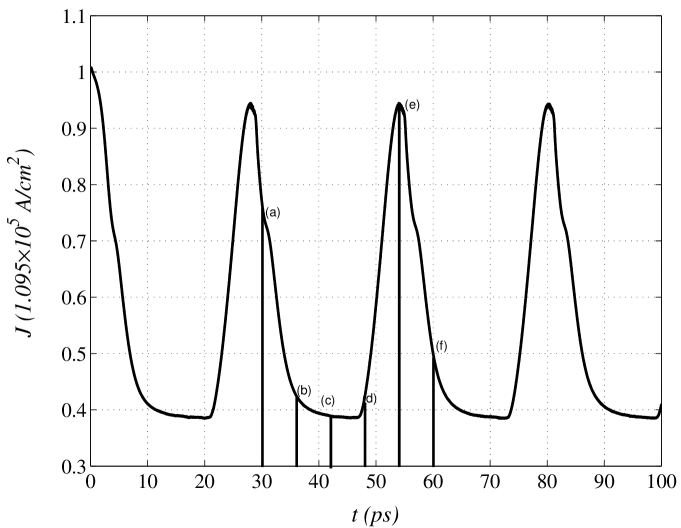
Figure 1: Total current density versus time plot exhibiting self-sustained oscillations. Units are written in parentheses. The oscillation period is 24 ps and the ratio between the maximum and the minimum current is 2.6. At the times marked (a) - (f) within one oscillation period (30, 36, 42, 48, 54 and 60 ps, respectively), we shall depict the electric field profile, the electron density profile, the distribution function and the density plots thereof in Figures 2, 8,  6 and 7, respectively.

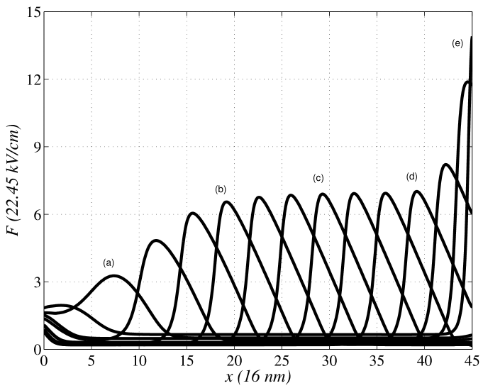
Figure 2: Electric field versus position at different times within one period of the oscillation. Far from the contacts, at time (c), the electric field pulse is 320 nm wide and 139 kV/cm tall. Thus it occupies about 45% of the SL extension. At time (e), the electric field has a maximum value of 312 kV/cm.

For these parameter values, we consider 140800 particles and a mesh of 440 grid points for $x$ and 80 points for $k$. The time step ($dt$) is $0.002$ ps. Figure 1 shows the self-oscillations of the current, and Figure 2 the corresponding electric field pulse at different times. We observe how the electric field pulses are periodically created at the injecting contact $x=0$, move to the end of the SL and disappear at the receiving contact. In Fig. 2, we have depicted the field profiles at the times marked (a) - (e) in Fig. 1. We observe that the total current density reaches its maximum value when the electric field pulse is about to disappear at the collector. The electric field as a function of time and position is shown in Figure 3, both during one oscillation period in Fig. 3(a) and during several periods in Fig. 3(b). The ratio from the maximum to the minimum current in Fig. 1 is 2.6 whereas the same ratio calculated by solving the drift-diffusion equation derived in [9] is 2.1 (cf. dashed line in Fig. 1(a) of [9]). Measured in units of $t_{0}$ (which has a different numerical value in [9]), the oscillation period is 104.3 in Fig. 1 whereas the drift-diffusion equation yields 113.8. Comparing Fig. 1(b) of [9] with our Fig. 2, we find that at the time (c) the solution of the BGK-Poisson equation produces a pulse far from the contacts which is $11\,x_{0}$ wide and $7\,F_{M}$ tall whereas the drift-diffusion equation yields a similar pulse which is $10.7\,x_{0}$ wide and $6.8\,F_{M}$ tall (cf. dashed line in Fig. 1(b) of [9]). Thus the agreement between the simulation of the BGK-Poisson system and that of the drift-diffusion equation is very good considering the approximations made in the derivation of the latter from the former.

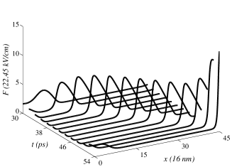
(a) (b)

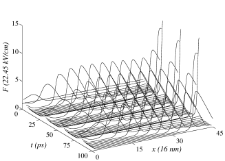
Figure 3: Evolution of the electric field $F(x,t)$ during (a) one period and (b) several periods of the self-oscillation.

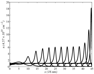
(a) (b)

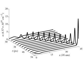
Figure 4: Electron density profiles during one oscillation period.

Figure 4 shows the dimensionless electron density. We see the profile during several times belonging to one oscillation period as a function of position in Fig. 4(a) and as a function of the time and position in Fig. 4(b). The electron density profile corresponding to an electric field pulse is that of a traveling dipole wave such that $n>1$ behind the peak of the electric field and $0<n<1$ ahead of the peak. Comparison with Fig. 3(a) shows that the local maximum of the electron density is reached somewhat later than the peak of the electric field pulse.

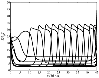
(a)     (b)

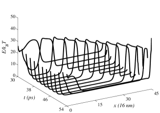
Figure 5: Nondimensional average energy profiles, $E/(k_{B}T),$ at different times of one oscillation period.

Figure 5(a) depicts the nondimensional average energy, $E/(k_{B}T)$ as a function of distance at different instants of one oscillation period. The average energy profile is pulse-like. Its local maximum is always quite close to the peak of the electric field during each oscillation period. Fig. 5(b) shows the average energy profile as a function of position and time during one oscillation period.

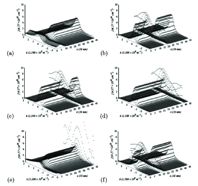
Figure 6: (a) - (f) Distribution function versus position and wave vector at the different times of one oscillation period as marked in Fig. 1.

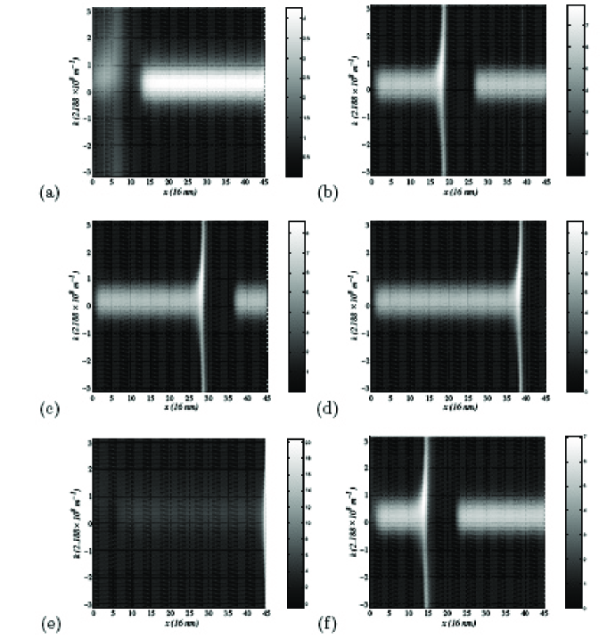
Figure 7: (a) - (f) Density plots of the distribution function versus position and wave vector at the different times of one oscillation period as marked in Fig. 1.

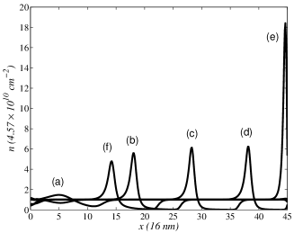
(a) (b)

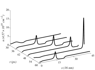
Figure 8: Electron density profile for the different times as marked in Fig. 1.

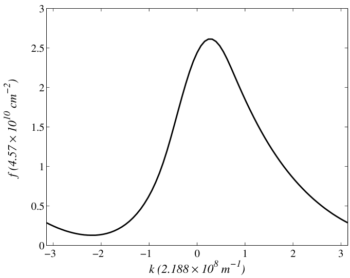
Figure 9: Distribution function versus wave vector at $t=0$ ps.

In Figure 6, we have depicted snapshots of the distribution function $f(x,k,t)$ for different times as marked in Fig. 1 ($30$ ps, $36$ ps, $42$ ps, $48$ ps, $54$ ps, $60$ ps) during one period of the self-oscillations. The structure of the distribution function is shown more clearly in the density plots depicted in Fig. 7 for the same times. The electron density profiles at the these times are shown in Figure 8. We observe that the distribution function has a local maximum at location of the peak of electron density. Similarly, $f$ and $n$ have local minima at the same positions. The distribution function has a local maximum at a positive $k$ (cf. Fig. 7), and this situation persists from the initial time onwards; cf. Figure 9.

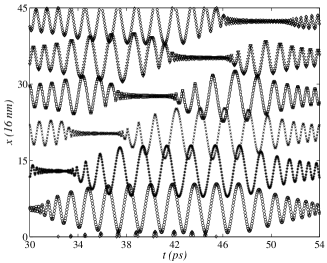
(a) (b)

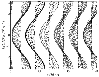
Figure 10: Time evolution of the position for six particles whose initial dimensionless wave vector is $-3.126$: (a) position vs time, (b) wave vector vs position for the same particles.

Figure 10(a) shows the time evolution of the position for six particles, whereas Figure 10(b) shows the wave vector vs position for the same particles. The motion of the particles is a superposition of an uniform motion and an oscillation about it. Comparing Figure 10(a) with Fig. 3(a), we observe that the particle positions oscillate with very small amplitudes when the electric field has a local maximum at their locations and these amplitudes become larger once the pulse has surpassed the particles. In contrast with these great changes in oscillation amplitude of the particle positions, the wave vectors of the particles oscillate with almost constant amplitudes, as shown in Fig. 10(b), 11 and 12. Since the evolution of the particle wave vector is more regular than the evolution of the particle position, we can save mesh points on the wave vectors. Recalling that the wave vector is a periodic variable, its boundary condition is as follows: when one particle goes out of the domain at $k=\pi$, it is reintroduced at $k=-\pi$. This condition can be readily observed in Figures 11 and 12.

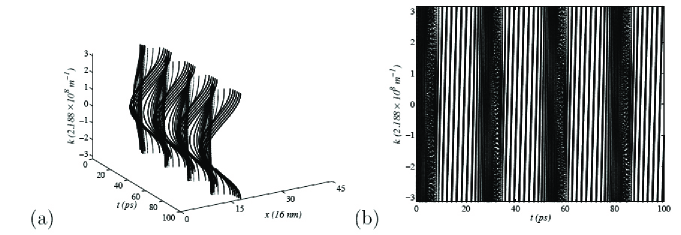
Figure 11: Time evolution of the particle with initial dimensionless position and wave vector $(13.986,-3.126)$ during several oscillation periods.

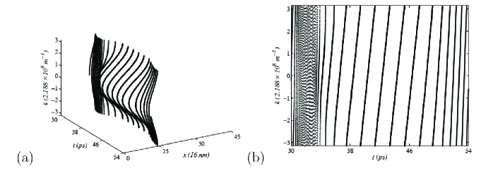
Figure 12: Time evolution of the particle with initial dimensionless position and wave vector $(13.986,-3.126)$ during one oscillation period.

6 Convergence of the method

We have checked the convergence of the method in terms of the number of particles $N$, mesh points $M_{x}$ and $M_{k}$, and time step $dt$. Since the Fermi-Dirac weights in (28) and the electric field in (29) have to be calculated by interpolation over mesh points, all these parameters are important for the convergence of the calculations over particles and of the calculations over the mesh. The physical parameters are the same as in the previous section.

Figure 13 shows the evolution of the current density for different number of particles $N$. We have kept the time step and the wave number mesh points fixed at the values $M_{k}=80$ and $dt=0.008$ ps. We observe that we need different $N$ for convergence of the calculation depending on the value of $M_{x}$. In Fig. 13(a), for $M_{x}=440$ position mesh points, we have chosen $N$ so that $N/(M_{x}M_{k})$ takes on the values 1.5, 1.84, 2.25 and 3, whereas in Fig. 13(b), $M_{x}=360$ and $N$ is chosen so that $N/(M_{x}M_{k})$ takes on the values 1.5, 2.25 and 3. We observe that for $dt=0.008$ ps and $N/(M_{x}M_{k})\geq 2.25$ the results do not change if we increase the number of particles. In particular, for $N=64800$, $N/(M_{x}M_{k})=1.84$ if $M_{x}=440$ and $N/(M_{x}M_{k})=2.25$ if $M_{x}=360$. In the first case shown in Fig. 13(a), we need more particles for the method to converge whereas in the second case, Fig. 13(b) shows that we do not improve our results by increasing $N$. The convergence range of $N/(M_{x}M_{k})$ depends slightly on the time step $dt$: if $dt=0.002$ ps, $M_{x}=440$, $M_{k}=80$, our calculations yield indistinguishable curves $J(t)$ for $N/(M_{x}M_{k})=3,\,4$, but not for $N/(M_{x}M_{k})=2.25$. Thus we have found that it is advisable to select $N$ so that $3\leq N/(M_{x}M_{k})\leq 4.5$: numerical results are indistinguishable when $N/(M_{x}M_{k})\geq 3$ and the computational cost is not very large if we keep $N/(M_{x}M_{k})\leq 4.5$.

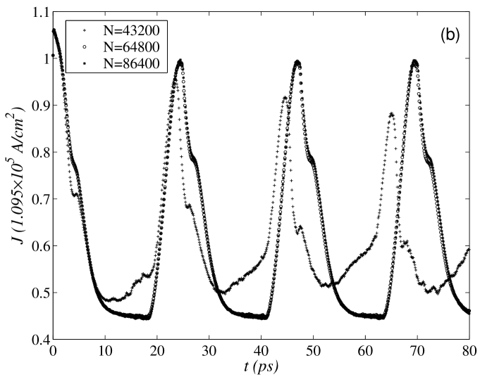
Figure 13: Current versus time for different number of particles $N$ when $M_{k}=80$ and $dt=0.008$ ps. (a) $M_{x}=440$ and (b) $M_{x}=360.$

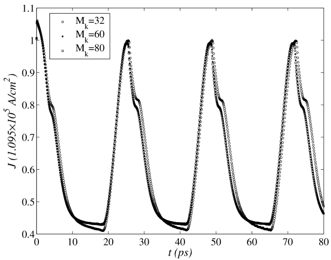
Figure 14: Current versus time for different number of wave vector mesh points when $M_{x}=520,$ $N=200000$ and $dt=0.008$ ps.

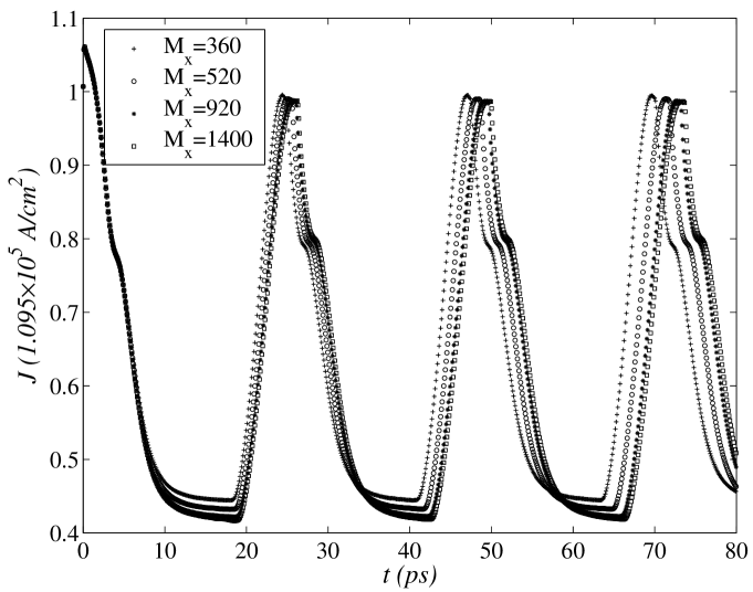
Figure 15: Current versus time for different number of position mesh points when $M_{k}=80,$ $N=480000$ and $dt=0.008$ ps.

Figures 14 and 15 show the evolution of the total current density in simulations having a different number of mesh points when the time step is $dt=0.008$ ps. In Fig. 14, different wave vector mesh points are considered for $M_{x}=520$ and $N=200000.$ We can check that we do not need to have a very fine grid in $k$ because we obtain the same results with $M_{k}=60$ and $M_{k}=80$. In Fig. 15, different numbers of position mesh points are considered for $M_{k}=80$ and $N=480000.$ For $M_{x}=920$ and larger our numerical curves overlap.

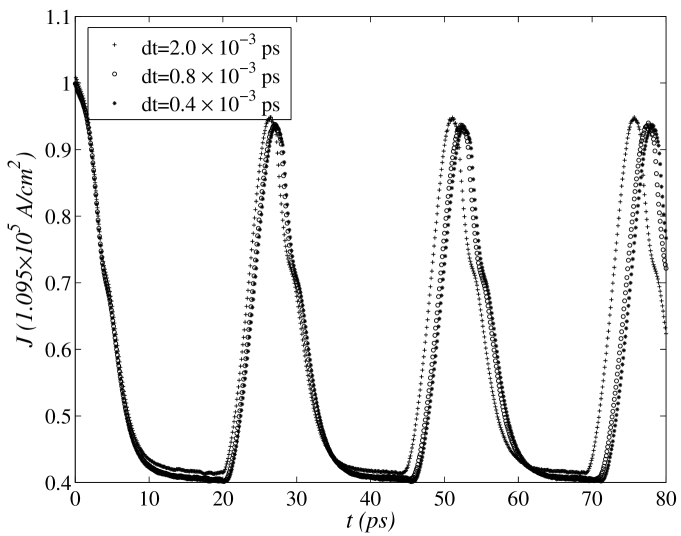
Figure 16: Current versus time for different time steps when $N=90000$, $M_{x}=260$ and $M_{k}=80$.

Lastly, Figure 16 shows the evolution of the total current density for different time steps in simulations with 90000 particles and 260 mesh grid points for the position and 80 for the wave vector. We observe that our results are similar for time steps $dt=8\times 10^{-4}$ ps and smaller.

Figures 14 to 16 show that the shape of $J(t)$ is similar for different mesh points and time steps: the device behavior is qualitatively correct even if we take fewer mesh points or larger time steps than needed to attain a numerically precise current vs time graph. Smaller $M_{k}$, $M_{x}$ and larger $dt$ result in slightly smaller oscillation periods and slightly larger oscillation amplitudes.

Our numerical simulations have been carried out using a Matlab code in a computer with a Genuine Intel(R) CPU T2050 @ 1.60GHz processor with a 1595 MHz speed. Several computation times for time steps $dt$ of 0.008 and 0.002 ps and 10000 time steps are shown in Table 2. Clearly, the time the computer takes to calculate one time step $dt$ decreases as the number of particles, $M_{x}$ or $M_{k}$ decrease. Except for the last row in Table 2, all rows satisfy $N/(M_{x}M_{k})\geq 2.25$, and the corresponding particle numbers and $x$ and $k$ mesh points produce accurate enough results.

$$\hskip-22.76219pt\begin{array}[]{c}\begin{array}[]{|c|c|c|c|c|c|}\hline\cr N&M_{x}&M_{k}&\frac{N}{M_{x}M_{k}}&dt\mbox{ (ps)}&\mbox{(C.T.)/\# steps (seconds)}\\ \hline\cr 480000&920&80&6.52&0.008&2.64\\ \hline\cr 480000&360&80&16.67&0.008&2.12\\ \hline\cr 200000&520&80&4.81&0.008&1.19\\ \hline\cr 200000&520&32&12.02&0.008&1.15\\ \hline\cr 140800&440&80&4.00&0.002&0.87\\ \hline\cr 105600&440&80&3.00&0.002&0.73\\ \hline\cr 79200&440&80&2.25&0.002&0.65\\ \hline\cr 52800&440&80&1.50&0.002&0.53\\ \hline\cr\end{array}\\ {\rm Table\,2:\,Computer\,time\,(C.T.).}\end{array}$$

7 Conclusion

We have proposed a deterministic weighted particle method to numerically solve for the first time the semiclassical Boltzmann-BGK-Poisson system of equations with periodic miniband energy dispersion relation. This system describes vertical electron transport in a GaAs/AlAs superlattice under dc voltage bias conditions. When using appropriate values for the injecting contact conductivity and voltage, we find a stable self-sustained oscillation of the current through the structure which corresponds to periodic nucleation of electric field pulses at the injecting contact that then move to the receiving contact. The pulses have a large electron density on their trailing edges which implies large gradients of the electric field there. These gradients are well resolved by particles having large weights there, which is one of the advantages of using the weighted particle numerical method. Our results agree with experimental observations [13, 4] and confirm the validity of the Chapman-Enskog perturbation method used to derive a drift-diffusion equation for high electric fields [3]. In fact, the electric field profile and the total current density obtained by numerically solving the the drift-diffusion equation [9] agree very well with the numerical solution of the kinetic equations obtained in the present work. Having solved the kinetic equations directly, we can obtain the evolution of the distribution function and its relevant moments such as electron density, current density and average energy. The present work paves the way to numerically solving interesting problems in nanoelectronics and spintronics that are described by related quantum kinetic equations with more than one miniband [2].

Acknowledgements: This work has been supported by the Ministry of Science and Innovation grants FIS2008-04921-C02-02 (EC and AC) and FIS2008-04921-C02-01 (LLB).

References

- [1] P.L. Bhatnagar, E.P. Gross, M. Krook, A model for collision processes in gases. I Small amplitude processes in charged and neutral one-component systems, Phys. Rev. 94 (1954) 511–525.
- [2] L.L. Bonilla, L. Barletti, M. Álvaro, Nonlinear electron and spin transport in semiconductor superlattices. SIAM J. Appl. Math. 69 (2008) 494–513.
- [3] L.L. Bonilla, R. Escobedo, A. Perales, Generalized drift-diffusion model for miniband superlattices, Phys. Rev. B 68 (2003) 241304(R) (4 pages).
- [4] L.L. Bonilla, H.T. Grahn, Nonlinear dynamics of semiconductor superlattices, Rep. Prog. Phys. 68 (2005) 577–683.
- [5] E. Cebrián, F.J. Mustieles, Deterministic Particle Simulation of Multiheterojunction Semiconductor Devices: The Semiclassical and Quantum Cases. Compel. 13 (1994) 717–725.
- [6] P. Degond, B. Niclot, Numerical Analysis of the Weighted Particle Applied to the Semiconductor Boltzmann Equation, Numer. Math. 55 (1989) 599–618.
- [7] F. Delaurens, F.J. Mustieles, A Deterministic Particle Method for Solving Kinetic Transport Equations: The Semiconductor Boltzmann Equation Case. SIAM J. Appl. Math. 52 (1992) 973–988.
- [8] L. Esaki and R. Tsu, Superlattice and negative differential conductivity in semiconductors. IBM J. Res. Develop. 14, 61-65 (1970).
- [9] R. Escobedo, L.L. Bonilla, Numerical methods for a quantum drift-diffusion equation in semiconductor physics. J. Math. Chem. 40 (2006) 3–13.
- [10] Y. Farjoun, B. Seibold, An exactly conservative particle method for one dimensional scalar conservation laws. J. Comput. Phys., to appear. See: ArXiv:0809.0726.
- [11] J. Feldmann, K. Leo, J. Shah, D. A. B. Miller, J. E. Cunnigham, T. Meier, G. von Plessen, A. Schulze, P. Thomas, and S. Schmitt-Rink, “Optical investigation of Bloch oscillations in a semiconductor superlattice”. Phys. Rev. B 46, 7252-7255 (1992).
- [12] R.R. Gerhardts, Effect of elastic scattering on miniband transport in semiconductor superlattices. Phys. Rev. B 48 (1993) 9178–9181.
- [13] K. Hofbeck, J. Grenzer, E. Schomburg, A.A. Ignatov, K.F. Renk, D.G. Pavel’ev, Yu. Koschurinov, B. Melzer, S. Ivanov, S. Schaposchnikov, P.S. Kop’ev, High-frequency self-sustained current oscillation in an Esaki-Tsu superlattice monitored via microwave emission, Phys. Lett. A 218 (1996) 349–353.
- [14] A.A. Ignatov, V.I. Shashkin, Bloch oscillations of electrons and instability of space-charge waves in semiconductor superlattices, Sov. Phys. JETP 66 (1987) 526–530 [Zh. Eksp. Teor. Fiz. 93 (1987) 935–943].
- [15] A. A. Ignatov, E.P. Dodin and V.I. Shashkin, Transient response theory of semiconductor superlattices: connection with Bloch oscillations. Mod. Phys. Lett. B 5, 1087-1094 (1991).
- [16] D. Issautier, Convergence of a weighted particle method to solve the Boltzmann (B.G.K.) equation, SIAM J. Numer. Anal. 33 (1996) 2099–2119.
- [17] C. Jacoboni, L. Reggiani, The Monte Carlo method for the solution of charge transport in semiconductors with applications to covalent materials. Rev. Mod. Phys. 55 (1983) 645–705.
- [18] H. Kroemer, Gunn effect — bulk instabilities. Chapter 2 of Topics in Solid State and Quantum Electronics, edited by W. D. Hershberger. Pages 20-98. John Wiley, N. Y. 1972.
- [19] S.A. Ktitorov, G.S. Simin, V.Ya. Sindalovskii, Bragg reflections and the high-frequency conductivity of an electronic solid-state plasma, Sov. Phys. Solid State 13 (1972) 1872–1874 [Fiz. Tverd. Tela 13 (1971) 2230–2233].
- [20] B. Niclot, P. Degond, F. Poupaud, Deterministic Particle Simulation of the Boltzmann Transport Equation of Semiconductors. J. Comput. Phys. 78 (1988) 313–349.
- [21] C. Zener, A theory of the electrical breakdown of solid dielectrics. Proc. R. Soc. London, Ser. A 145, 523-529 (1934).