Diffusive dynamics on weighted networks

Mean-field diffusive dynamics on weighted networks

Abstract

Diffusion is a key element of a large set of phenomena occurring on natural and social systems modeled in terms of complex weighted networks. Here, we introduce a general formalism that allows to easily write down mean-field equations for any diffusive dynamics on weighted networks. We also propose the concept of annealed weighted networks, in which such equations become exact. We show the validity of our approach addressing the problem of the random walk process, pointing out a strong departure of the behavior observed in quenched real scale-free networks from the mean-field predictions. Additionally, we show how to employ our formalism for more complex dynamics. Our work sheds light on mean-field theory on weighted networks and on its range of validity, and warns about the reliability of mean-field results for complex dynamics.

I Introduction

Weighted networks represent the natural framework to describe natural, social, and technological systems, in which the intensity of a relation or the traffic between elements are important parameters Barthelemy:2005 ; barrat07:_archit . In general terms, weighted networks (WN) are an extension of the concept of network or graph Dorogovtsev:2003 ; Albert:2002 , in which each edge between vertices $i$ and $j$ has associated a variable, called weight, taking the form $\omega_{ij}=g(i,j)a_{ij}$, where $a_{ij}$ is the adjacency matrix and $g(i,j)$ is a function of $i$ and $j$ newman2004awn . Practical realizations of weights in real networks range from the number of passengers traveling yearly between two airports in the airport network Barrat:2004b , to the intensity of predator-prey interactions in ecosystems krause03 or the traffic measured in packets per unit time between routers in the Internet RomusVespasbook . A non-weighted network can thus be understood as a binary network, in which $\omega_{ij}=a_{ij}$, taking the value $1$ when vertices $i$ and $j$ are connected, and zero otherwise. Leaving aside the issue of the proper characterization of the topological observables associated to networks and their weighted extensions barrat07:_archit ; Barrat:2004b ; Barthelemy:2005 ; serrano06:_correl ; ahnert:016101 ; garlaschelli:038701 , a most relevant aspect of WN is the effect of the weight distribution and structure on the properties of dynamical processes taking place on top of them PhysRevE.65.027103 ; PhysRevLett.95.098701 ; wu07:_walks ; karsai:036116 ; 0256-307X-22-2-068 ; colizza07:_invas_thres ; ISI:000268327600005 ; yang:046108 . These can have an impact in problems ranging from the information transport in mobile communication networks onnela2007sat , the risks of congestion on Internet huberman1997sda , the disease spreading in the air transportation network colizza06:prediction or biological issues such as the role of weak interactions in ecological networks berlow1999sew .

In general, the theoretical understanding of dynamical processes on networks is based at a mesoscopic level on the heterogeneous mean-field (HMF) approximation and the annealed network approach dorogovtsev07:_critic_phenom ; barrat08:_dynam , which assume that the degree is the only relevant variable characterizing the vertices, and that dynamical fluctuations are not relevant. All dynamical variables can therefore be described in terms of deterministic rate equations, as a function of time and degree. Here, we develop the HMF theory for general local diffusive processes on WN by extending the annealed network approximation dorogovtsev07:_critic_phenom to the weighted case. We also define the concept of annealed weighted network, in which HMF theory is exact. We show the validity of our approach by obtaining an exact mean-field solution of the paradigmatic random walk process on WN. A comparison with numerical simulations allows to set the limits of validity of HMF on quenched weighted networks, showing also that it yields in some cases severely incorrect results. Finally, we present an example of the application of the annealed weighted network approximation to more complex dynamics on WN to obtain HMF rate equations.

Our approach allows for a straightforward mean-field description of diffusive dynamics on weighted networks, but at the same time calls for a careful interpretation of mean-field results on quenched networks, an issue already discussed in the non-weighted case Castellano:2006 ; hong07:_comment ; castellano07:_reply ; Castellano:2008 . HMF indeed does not take into account the quenched structure of the considered network, which however can play a fundamental role inducing strong deviations even in the apparently safe case in which only degree dependent weights are present. This should be recalled when mean-field predictions are to be compared with numerical simulations or used as a baseline to make predictions on processes on real weighted networks.

II Annealed weighted network approximation

II.1 Annealed network approximation in binary networks

The HMF theory for dynamical processes on binary complex networks is ultimately based on the annealed network approach dorogovtsev07:_critic_phenom , that consists in replacing the adjacency matrix $a_{ij}$, which in a real quenched network is composed by zeros and ones at fixed positions, by the probability $\bar{a}_{ij}$ that vertices $i$ and $j$ are connected. At a statistical degree coarse-grained level, we can replace $a_{ij}$ by the ensemble average $\bar{a}(k_{i},k_{j})$ boguna09:_langev , defined as the probability that two vertices of degree $k_{i}$ and $k_{j}$ are connected; that is, by the degree class average (for undirected networks)

$$\bar{a}(k,k^{\prime})=\frac{1}{NP(k)}\frac{1}{NP(k^{\prime})}\sum_{i\in k}\sum_{j\in k^{\prime}}a_{ij}\equiv\frac{kP(k^{\prime}|k)}{NP(k^{\prime})},$$ (1)

where $i\in k$ denotes a sum over the set of vertices of degree $k$, $P(k)$ is the degree distribution (probability that a randomly chosen vertex is connected with other $k$ vertices) Albert:2002 and $P(k^{\prime}|k)$ is the conditional probability that a vertex of degree $k$ is connected to a vertex of degree $k^{\prime}$ Pastor-Satorras:2001 . In other words, the original network is replaced by a fully connected graph in which each edge has associated a connection probability $\bar{a}(k_{i},k_{j})$ that depends only on the degree of its endpoints. The annealed network approach can be directly applied in calculations at the microscopic (vertex) level or, otherwise, fruitfully extended to a more intuitive mesoscopic (degree class) level. In the case of diffusive dynamics, the reasoning runs as follows. In diffusive dynamics, particles or interactions move from one vertex to another by jumping to a randomly chosen nearest neighbor. Therefore, the probability that vertex $i$ interacts with vertex $j$, $P(i\to j)$ (the propagator of the diffusive interaction), is given by

$$P(i\to j)=\frac{a_{ij}}{k_{i}}\equiv\frac{a_{ij}}{\sum_{r}a_{ir}}.$$ (2)

Performing a coarse-graining in degree classes, we can define the probability that a vertex of degree $k$ interacts with a vertex of degree $k^{\prime}$, namely

$$P(k\to k^{\prime})=\frac{[NP(k)]^{-1}\sum_{i\in k}\sum_{j\in k^{\prime}}a_{ij}}{[NP(k)]^{-1}\sum_{i\in k}\sum_{r}a_{ir}}\equiv P(k^{\prime}|k),$$ (3)

where we have used Eq. (1). With this concept in hand, writing down the HMF rate equations for any diffusive dynamical process turns out to be straightforward dorogovtsev07:_critic_phenom .

Equation (3) also encodes the idea of an annealed network boguna09:_langev ; gil05:_optim_disor ; weber07:_gener ; Castellano:2008 ; stauffer_annealed2005 . In opposition to quenched networks, in which edges are frozen between pairs of vertices, annealed networks are dynamical objects, changing in time over a certain timescale $\tau_{N}$, while keeping constant the degree distribution $P(k)$ and correlations $P(k^{\prime}|k)$. When the network time scale is very small, $\tau_{N}\to 0$, connections in the network are completely reshuffled between any two microscopic steps of the dynamics. In this case, the annealed network is completely defined by the quantities $P(k)$ and $P(k^{\prime}|k)$. From a computational point of view, a diffusive dynamics is easily simulated in these networks, by assigning to each vertex of degree $k$ nearest neighbors that are randomly selected among all the vertices in the network, according to the probability $P(k\to k^{\prime})=P(k^{\prime}|k)$. In the case of degree uncorrelated networks, this interaction probability simplifies further to $k^{\prime}P(k^{\prime})/\left<k\right>$, so that nearest neighbors are randomly chosen with probability proportional to their degree. Due to the very definition of the annealed network approach, HMF theory is exact in annealed networks .

II.2 Extension to weighted networks

We now generalize the annealed network approach to the weighted case. Assuming that the diffusion process is local (depends only on the departing and arriving vertices), the most general way to take into account weights in the random walk is to define the probability that a vertex $i$ interacts with vertex $j$ as a general function of the weight $\omega_{ij}$. The normalized form of this probability will be

$$P_{w}(i\to j)=\frac{F[\omega_{ij}]}{\sum_{r}F[\omega_{ir}]}.$$ (4)

The only restriction we impose to the function $F[x]$ is that $F[0]=0$, in order to avoid diffusion between disconnected vertices (i.e., with $a_{ij}=0$). This implies that we can write

$$F[\omega_{ij}]\equiv F[g(i,j)]a_{ij}.$$ (5)

At a mesoscopic level, we again consider the average probability of interaction of a vertex $k$ with a vertex $k^{\prime}$, that is defined, in analogy with Eq. (3), by

$$P_{w}(k\to k^{\prime})=\frac{[NP(k)]^{-1}\sum_{i\in k}\sum_{j\in k^{\prime}}F[\omega_{ij}]}{[NP(k)]^{-1}\sum_{i\in k}\sum_{r}F[\omega_{ir}]}$$ (6)

At the HMF level, where the vertices’s degrees are the only relevant topological variables, this expression can be simplified considering that the dependence of the weight on the vertices at the endpoints of each edge can be expressed as a function of the corresponding degrees, that is, $\omega_{ij}=\bar{g}(k_{i},k_{j})a_{ij}$. Using this relation, we have from Eqs. (5) and (1)

$$\frac{\sum_{i\in k}\sum_{j\in k^{\prime}}F[\omega_{ij}]}{NP(k)} = \frac{\sum_{i\in k}\sum_{j\in k^{\prime}}F[g(i,j)]a_{ij}}{NP(k)}=F[\bar{g}(k,k^{\prime})]\frac{\sum_{i\in k}\sum_{j\in k^{\prime}}a_{ij}}{NP(k)}\equiv kF[\bar{g}(k,k^{\prime})]P(k^{\prime}|k),$$ (7)

$$\frac{\sum_{i\in k}\sum_{r}F[\omega_{ir}]}{NP(k)} = \frac{\sum_{i\in k}\sum_{r}F[g(i,j)]a_{ij}}{NP(k)}=\sum_{q}F[\bar{g}(k,q)]\frac{\sum_{i\in k}\sum_{j\in q}a_{ij}}{NP(k)}\equiv k\sum_{q}F[\bar{g}(k,q)]P(q|k).$$ (8)

From this expressions, we finally obtain the degree coarse-grained weighted propagator

$$P_{w}(k\to k^{\prime})=\frac{F[\bar{g}(k,k^{\prime})]P(k^{\prime}|k)}{\sum_{q}F[\bar{g}(k,q)]P(q|k)},$$ (9)

satisfying the normalization condition $\sum_{k^{\prime}}P_{w}(k\to k^{\prime})=1$.

Simpler expressions for the weighted propagator can be obtained if we consider a linear diffusion process colizza07:_invas_thres ; wu07:_walks , proportional to the weight $\omega_{ij}$, in which $F(x)=x$. Furthermore, considering weights that are symmetric multiplicative functions of the degrees at the edges’ endpoints, namely $\bar{g}(k,k^{\prime})\equiv\bar{g}_{s}(k)\bar{g}_{s}(k^{\prime})$ (as is the case, for example, in the airport transportation network Barrat:2004b ), and a degree uncorrelated network, with $P(k^{\prime}|k)=k^{\prime}P(k^{\prime})/\left<k\right>$, we are led to the simple expression

$$P_{w}(k\to k^{\prime})=\frac{k^{\prime}\bar{g}_{s}(k^{\prime})P(k^{\prime})}{\langle{k\bar{g}_{s}(k)}\rangle},$$ (10)

where we define $\langle{G(k)}\rangle\equiv\sum_{k}G(k)P(k)$.

Writing the mean-field rate equations for most diffusive dynamical processes on WN is now easy: The analytics describing the dynamics on simple binary networks can be generalized to the weighted case simply by replacing the propagator $P(k\to k^{\prime})$ with $P_{w}(k\to k^{\prime})$.

The spirit in which the HMF rate equations are constructed leads also to introduce the concept of an annealed weighted network. In this case, in the event of an interaction, a vertex of degree $k$ chooses as the interaction target a vertex of degree $k^{\prime}$, randomly selected among all vertices in the network with probability $P_{w}(k\to k^{\prime})$. Therefore, an annealed weighted network can be understood as an annealed binary network, which is completely reshuffled between dynamic time steps, preserving its degree distribution $P(k)$ and an effective degree correlation pattern given by $P_{\mathrm{eff}}(k^{\prime}|k)\equiv P_{w}(k\to k^{\prime})$. Again, in the case of linear diffusion in a degree uncorrelated network with symmetric multiplicative weights, this connection probability simplifies to $k^{\prime}\bar{g}_{s}(k^{\prime})P(k^{\prime})/\langle{k\bar{g}_{s}(k)}\rangle$, so that the interacting vertex is chosen with probability proportional to $k\bar{g}_{s}(k)$. Simulations run on such networks are described exactly by weighted HMF rate equations. Quenched WN can in principle determine different behaviors, and, as we will see below, this is in fact the case.

III Random walks on weighted networks

III.1 Weighted heterogeneous mean-field solution

To check the application of the formalism derived above, let us consider as an example the simple yet paradigmatic random walk process noh04:_random_walks_compl_networ . This is defined by a walker that, located on a given vertex of degree $k$ at time $t$, hops to one of the $k$ neighbors of that vertex at time $t+1$, randomly chosen with probability depending on the weights connecting the vertices. The simplicity of this problem allows to solve it exactly for certain forms of the weight structure wu07:_walks ; fronczak:016107 , following the master equation approach developed in Ref. noh04:_random_walks_compl_networ . Here we focus on the application of the simpler HFM in the most general case, which provides results for any weight pattern.

To construct the appropriate HMF rate equation, we consider the probability $R_{k}(t)$ that the walker is in any vertex of degree $k$, which fulfills the master equation

$$\dot{R}_{k}(t) = -\sum_{k^{\prime}}R_{k}(t)P_{w}(k\to k^{\prime})+\sum_{k^{\prime}}P_{w}(k^{\prime}\to k)R_{k^{\prime}}(t)$$ (11)

$$= R_{k}(t)+\sum_{k^{\prime}}P_{w}(k^{\prime}\to k)R_{k^{\prime}}(t).$$

The first term in Eq. (11) represents the outflow of probability due to walkers abandoning vertices of degree $k$, while the second term represents walkers arriving to vertices of degree $k$ from vertices of degree $k^{\prime}$, following a weighted random step. In the steady state this equation takes the iterative form

$$R_{k}=\sum_{k^{\prime}}P_{w}(k^{\prime}\to k)R_{k^{\prime}}.$$ (12)

Interpreted in terms of a Markov process durret99:_essen , the steady state solution is given, for any degree correlation and weight pattern, by the expression

$$R_{k}=\lim_{n\to\infty}P^{(n)}_{w}(k\to k),$$ (13)

where $P^{(n)}_{w}$ is the $n$-th power of the probability $P_{w}(k\to k^{\prime})$, considered as a matrix. Explicit solutions in the steady state can be found for some weight patterns by imposing the detailed balance condition $R_{k}P_{w}(k\to k^{\prime})=R_{k^{\prime}}P_{w}(k^{\prime}\to k)$ durret99:_essen , which ensures a solution of Eq. (12). From this condition we obtain, for a general diffusion process,

$$\frac{R_{k}}{R_{k^{\prime}}} = \frac{P_{w}(k^{\prime}\to k)}{P_{w}(k\to k^{\prime})}$$ (14)

$$\equiv \frac{F[\bar{g}(k^{\prime},k)]kP(k)}{F[\bar{g}(k,k^{\prime})]k^{\prime}P(k^{\prime})}\frac{\sum_{q}F[\bar{g}(k,q)]P(q|k)}{\sum_{q}F[\bar{g}(k^{\prime},q)]P(q|k^{\prime})},$$

where in the last equality we have used the degree detailed balance condition $k^{\prime}P(k^{\prime})P(k|k^{\prime})=kP(k)P(k^{\prime}|k)$ Boguna:2002 . Then, for symmetric weights $\omega_{ij}=\omega_{ji}$, or, at the degree level, $\bar{g}(k,k^{\prime})\equiv\bar{g}_{s}(k,k^{\prime})=\bar{g}_{s}(k^{\prime},k)$, we obtain the normalized probability

$$fR_{k}=\frac{kP(k)\sum_{q}F[\bar{g}_{s}(k,q)]P(q|k)}{\sum_{k^{\prime}}\sum_{q}k^{\prime}P(k^{\prime})F[\bar{g}_{s}(k^{\prime},q)]P(q|k^{\prime})}.$$ (15)

If the weights only depend on the first vertex in the edge, that is, $\omega_{ij}=g_{1}(i)a_{ij}$ or $\bar{g}(k,k^{\prime})\equiv\bar{g}_{1}(k)$, the effect of weights effectively vanishes and we recover diffusion in a binary network noh04:_random_walks_compl_networ ,

$$R_{k}=\frac{kP(k)}{\sum_{k^{\prime}}k^{\prime}P(k^{\prime})}$$ (16)

Finally, if the weights only depend on the second vertex in the edge, that is, $\omega_{ij}=g_{2}(j)a_{ij}$ or $\bar{g}(k,k^{\prime})\equiv\bar{g}_{2}(k^{\prime})$, then we obtain

$$R_{k}=\frac{kP(k)F[\bar{g}_{2}(k)]\sum_{q}F[\bar{g}_{2}(q)]P(q|k)}{\sum_{k^{\prime}}\sum_{q}k^{\prime}P(k^{\prime})F[\bar{g}_{2}(k^{\prime})]F[\bar{g}_{2}(q)]P(q|k^{\prime})}.$$ (17)

Noticeably, results (15) and (17) coincide if diffusion is linear, $F(x)=x$, and the weights are symmetric and multiplicative, $\bar{g}_{s}(k,k^{\prime})=\bar{g}_{s}(k)\bar{g}_{s}(k^{\prime})$, recovering the results reported in wu07:_walks ; fronczak:016107 .

Further quantities can be analogously computed with ease in the annealed WN approximation. For example, the coverage $S(t)$ montroll:167 ; stauffer_annealed2005 ; baronchelli08:_random , defined as the average number of different vertices visited by the walker at time $t$, can be computed as follows. Let us define $s_{k}(t)=v_{k}(t)/[NP(k)]$ as the fraction of vertices of degree $k$ visited by the random walker, $v_{k}(t)$ being total number of such vertices. From here, we have $S(t)=N\sum_{k}P(k)s_{k}(t)$. The quantity $v_{k}(t)$ increases in time as the random walk arrives to vertices that have never been visited. Therefore, at a mean-field level, it fulfills the rate equation baronchelli08:_random

$$\dot{v}_{k}(t)=[1-s_{k}(t)]\sum_{k^{\prime}}P_{w}(k^{\prime}\to k)R_{k^{\prime}}(t).$$ (18)

Dividing this equation by $NP(k)$ and using Eq. (9), we are led in the general case to

$$\dot{s}_{k}(t)=[1-s_{k}(t)]k\sum_{k^{\prime}}\frac{F[\bar{g}(k^{\prime},k)]P(k^{\prime}|k)}{Nk^{\prime}P(k^{\prime})\sum_{q}F[\bar{g}(k^{\prime},q)]P(q|k^{\prime})}R_{k^{\prime}}(t).$$ (19)

Assuming now that $R_{k}(t)$ reaches its steady state in a very short time, of order $1$, we can substitute the steady state value $R_{k}$ into Eq. (19) and integrate it, with the initial condition $s_{k}(0)=0$. For symmetric weights, Eq. (15) the integrations leads to the result

$$s_{k}(t)=1-\exp\left\{-t\;\frac{k\sum_{k^{\prime}}F[\bar{g}_{s}(k^{\prime},k)]P(k^{\prime}|k)}{N\sum_{k^{\prime\prime}}\sum_{q}k^{\prime\prime}P(k^{\prime\prime})F[\bar{g}_{s}(k^{\prime\prime},q)]P(q|k^{\prime\prime})}\right\}.$$ (20)

Moreover, straightforward mean-field arguments saramaki2004sfn ; baronchelli2003rsa ; baronchelli08:_random provide an expression for the mean first-passage time (MFPT) $\tau_{k}$, defined as the average time that a walker takes to arrive to a given vertex of degree $k$, starting from a randomly chosen initial vertex noh04:_random_walks_compl_networ . Let us define the occupation probability $\rho_{k}(t)=R_{k}(t)/[NP(k)]$ as the probability that the walker is at a given vertex of degree $k$. Thus, the probability for the walker to arrive at a vertex $i$, in a hop following a randomly chosen weighted edge, is given by $q(i)=\rho_{k_{i}}(t)$. Therefore, the probability of arriving at vertex $i$ for the first time after $t$ hops is $P_{a}(i;t)=[1-q(i)]^{t-1}q(i)$. The MFPT to vertex $i$ can thus be estimated as the average

$$\tau_{k_{i}}=\sum_{t}tP_{a}(i;t)=\frac{1}{q(i)}.$$ (21)

We have thus that the MFPT is proportional to the inverse of the steady state probability, $R_{k}$, namely

$$\tau_{k}=\frac{NP(k)}{R_{k}}.$$ (22)

This simple HMF approximation can be improved by the inclusion of sub-leading terms using more formal techniques noh04:_random_walks_compl_networ ; fronczak:016107 .

III.2 Dynamics on quenched weighted networks

The weighted HMF expressions obtained above will exactly match, by definition, the results of simulations on annealed WN. A different issue is, however, their validity for real quenched WN, in particular for networks with a scale-free degree distribution, $P(k)\sim k^{-\gamma}$ Dorogovtsev:2003 ; Albert:2002 . The question of the non mean field behavior of dynamical processes on binary networks has been already pointed out in the literature Castellano:2006 ; 1742-5468-2006-05-P05001 . As we will see, the situation can get even worse in the case of WN.

We consider as a particular example the case of liner diffusion on symmetric multiplicative weighted networks, with weight intensity $\bar{g}_{s}(k)=k^{\theta}$, typical of some real systems such as the airport network Barrat:2004b . In the limit of large positive $\theta$, in an annealed WN we would expect the random walker to reach the largest hub in the first time step, and then stay there forever . In a quenched WN, on the other hand, the walker is expected to commute forever between the first encountered pair of vertices who have the property of being reciprocally the highest degree neighbor of each other. In order to explore quantitatively this intuitive disagreement, we have performed numerical simulations of random walks in degree uncorrelated and multiplicative scale-free WN, with weight intensity $\bar{g}_{s}(k)=k^{\theta}$ and linear diffusion, which yield the HMF results

$$\tau_{k}=\frac{1}{\rho_{k}}=\frac{N\langle{k^{1+\theta}}\rangle}{k^{1+\theta}},$$ (23)

$$1-\frac{S(t)}{N}=\mathcal{F}_{\gamma,\theta}\left(\frac{t}{N\langle{k^{1+\theta}}\rangle}\right),$$ (24)

where $\mathcal{F}_{\gamma,\theta}(x)$ is a scaling function depending on $\gamma$ and $\theta$. Uncorrelated scale-free quenched networks with any degree exponent $\gamma$ are created using the Uncorrelated Configuration Model (UCM) Catanzaro:2005 , characterized by a hard cut-off $k_{c}=\sqrt{N}$, preventing the generation of correlations for $\gamma<3$. Random walks are performed by moving the walker from its present position $i$ to a nearest neighbor $j$, chosen with probability

$$P(i\to j)=\frac{k_{j}^{\theta}a_{ij}}{\sum_{q}k_{q}^{\theta}a_{iq}}.$$ (25)

On annealed WN, on the other hand, the next step of the walk is a vertex $j$, randomly chosen among all vertices in the network with probability proportional to $k_{j}^{1+\theta}$, see Eq. (10). In our simulations we keep fixed a degree exponent $\gamma=2.5$ and a minimum degree of the network $m=4$.

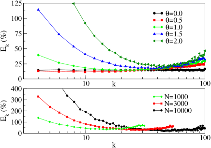
Figure 1: (Color Online) Top: Relative error between the theoretical HMF prediction Eq. (23) and numerical simulations for the MFPT in quenched scale-free WN of size $N=10^{4}$ and $\gamma=2.5$. Bottom: Relative error for $\theta=2.5$ and different network sizes.

We first study the validity of the weighted HMF prediction for the MFPT, by examining the differences between the theoretical expression $\tau_{k}^{th}$, Eq. (23), and the numerical result, $\tau_{k}^{num}$. In particular, we focus on the relative error as a function of the degree, defined as

$$E_{k}=\frac{\tau_{k}^{num}-\tau_{k}^{th}}{\tau_{k}^{th}}.$$ (26)

Fig. 1(top) shows the numerical evaluation of this function in quenched scale-free WN of fixed size $N=10^{4}$, for different values of $\theta$ . For $\theta=0$, corresponding to a binary network, we recover a constant baseline error of about $15\%$, as already reported in the literature baronchelli2003rsa . As $\theta$ increases, the numerical results start to deviate from the HMF prediction, the error being larger for small degrees and also increasing for large $k$. The error in the estimate of the weighted HMF theory also increases when increasing the system size, as can be seen from Fig. 1(bottom).

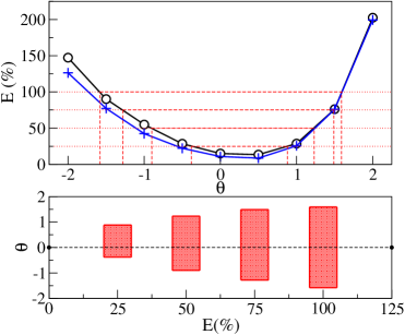
Figure 2: (Color Online) Top: Average error as a function of $\theta$ in quenched WN of size $N=10^{4}$ and $\gamma=2.5$ for the simple HMF estimate (circles), Eq. (23), and a more refined approximation (crosses), Eq. (27). Bottom: Range of $\theta$ values yielding an average error $E$ smaller than a given value for the HMF estimate.

In order to provide an estimate of the range of validity of the HMF approximation, in Fig. 2 we explore the average error as a function of $\theta$, $E=\sum_{k}P(k)E_{k}$. As we can see from Fig. 2(top), for the particular value $\gamma=2.5$ considered, the error is minimal, compatible with the baseline of $15\%$, in the interval $\theta\in[0,0.5]$, while it increases for values of $\theta$ outside this interval. In Fig. 2(top) we additionally compare the performance of the HMF prediction with a more elaborate estimate of the MFPT obtained by the master equation technique, namely fronczak:016107

$$\tau_{k}^{\prime}\simeq\frac{N\langle{k^{1+\theta}}\rangle}{k^{1+\theta}}+\frac{N\langle{k}\rangle^{2}}{k\langle{k^{2}}\rangle}-2.$$ (27)

As we can see, Eq. (27) fares slightly better for $\theta<0$, but the HMF result remains a fairly good first order approximation.

This kind of plot can be used to estimate the range of values of $\theta$ for which the weighted HMF approximation provides a correct result within an accepted maximum tolerable error, see Fig. 2(bottom). Thus, for example, a deviation smaller than a $50\%$ in scale-free networks with $\gamma=2.5$ is achieved for values of $\theta\in[-0.9,1.2]$. Outside this range, other more sophisticated approaches should be followed.

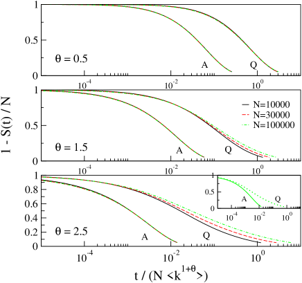
Figure 3: (Color Online) Data collapse of the network coverage, as given by Eq. (24), in annealed ($A$) and quenched ($Q$) scale-free WN, with $\gamma=2.5$ for different values of $\theta$ and network sizes. Curves shifted on the horizontal axis for clarity. Inset: Unshifted curves for $\theta=2.5$ and $N=10^{5}$ for annealed ($A$, continuous line) and quenched ($Q$, dotted line) WN.

Concerning the results for the network coverage $S(t)$, a direct comparison with Eq. (24) is not feasible, since the exact form of the function $\mathcal{F}_{\gamma,\theta}(x)$ depends on several approximations (steady state approximation in Eq. (20), continuous degree approximations, etc.). We therefore take as the main weighted HMF prediction the scaling form in Eq. (24), which we check by means of a data collapse analysis: If Eq. (24) is correct, we expect that plots of $1-S(t)/N$ as a function of $t/(N\langle{k^{1+\theta}}\rangle)$ will collapse onto the universal function $\mathcal{F}_{\gamma,\theta}(x)$ when plotted for different values of N. In Fig. 3 we compare the results of simulations on quenched weighted networks with simulations in the corresponding annealed ones, for different values of $\theta$. For small values of $\theta$ (i.e. smaller than $0.5$), we observe a perfect agreement in both sets of simulations with the weighted HMF prediction. Again, however, the perfect collapse of the annealed case contrasts with the large deviations shown by quenched networks for large values of $\theta$, outside the regime of validity of the weighted annealed network approximation.

The reason for the failure of weighted HMF theory in the random walk case is easy to understand. For positive $\theta$, a quenched topology reduces the accessibility of the network by trapping the walker in pairs of adjacent high degree vertices nodes and, at the same time, slows down the exploration of the network due to the trapping effect of high degree vertices carmi:066111 . These effects, which are stronger for large $\theta$, explain the large MFPT observed for small and large degree, Fig. 1(top), as well as the larger times needed to reach a fixed coverage, Fig. 3. For negative $\theta$, on the other hand, the walker is biased towards small degree vertices, missing thus the hubs that provide connectivity to far away regions in the network adamic01 .

IV General dynamical processes

As we have pointed out in Sec. II, the annealed weighted network approximation can be easily applied to general diffusive processes in weighted networks to obtain an approximate HMF solution. Within this framework, the weighted HMF rate equations are obtained from the ones on binary networks by substituting the binary propagator by the weighted one $P_{w}(k\to k^{\prime})$, Eq. (9).

As a case example of application, we will consider here the case of the contact process (CP) Marro , whose dynamics on a network is defined as follows Castellano:2006 : An initial fraction $\rho_{0}$ of vertices is randomly chosen and occupied by a particle. The time evolution of the process runs as follows: At each time step $t$, a particle in a vertex $i$ is chosen at random. With probability $p$, this particle disappears. With probability $1-p$, on the other hand, the particle may generate an offspring. To do so, a vertex $j$, nearest neighbor of the vertex $i$, is chosen. If vertex $j$ is occupied by a particle, nothing happens; if it is empty, a new particle is created on $j$. In any case, time is updated as $t\to t+1/n(t)$, where $n(t)$ is the number of particles present at the beginning of the time step. In a binary network, the second vertex $j$ is chosen uniformly at random among all neighbors of $i$, i.e. with probability $1/k_{i}$. In a weighted network, on the other hand, it is selected with probability depending on $\omega_{ij}$.

The key point in the HMF analysis of the CP is the probability $\rho_{k}(t)$ that a vertex of degree $k$ is occupied by a particle at time $t$ Castellano:2006 ; Castellano:2008 . To write the HMF equation for this quantity it is useful to focus instead on the number of occupied vertices of degree $k$, $n_{k}(t)$, which is related to $\rho_{k}(t)$ by

$$\rho_{k}(t)=\frac{n_{k}(t)}{NP(k)}.$$ (28)

The rate equation for $n_{k}(t)$ is easy to obtain by means of mean-field arguments Castellano:2006 ; marianproc , leading to

$$\dot{n}_{k}(t)=-pn_{k}(t)+(1-p)[1-\rho_{k}(t)]\sum_{k^{\prime}}P_{w}(k^{\prime}\to k)n_{k^{\prime}}(t).$$ (29)

The first term comes from particles disappearing from vertices of degree $k$ with probability $p$; the second term correspond to the offsprings of particles in connected vertices of degree $k^{\prime}$ (with probability $1-p$), arriving to vertices of degree $k$ which are empty (with probability $1-\rho_{k}(t)$). Dividing Eq. (29) by $NP(k)$, substituting the expression of the weighted propagator Eq. (9) and applying the degree detailed balance condition Boguna:2002 we obtain the general weighted HMF equation for the CP

$$\dot{\rho}_{k}(t)=-\rho_{k}(t)+\lambda k[1-\rho_{k}(t)]\sum_{k^{\prime}}\frac{F[\bar{g}(k^{\prime},k)]P(k^{\prime}|k)}{k^{\prime}\sum_{q}F[\bar{g}(k^{\prime},q)]P(q|k^{\prime})}\rho_{k^{\prime}}(t).$$ (30)

In this last equation, we have performed a rescaling of time, and defined the parameter $\lambda=(1-p)/p$. For symmetric multiplicative weights of the form $\bar{g}(k,k^{\prime})=\bar{g}_{s}(k)\bar{g}_{s}(k^{\prime})$, and assuming linear diffusion a degree uncorrelated network, we are led to the simplified equation

$$\dot{\rho}_{k}(t)=-\rho_{k}(t)+\lambda[1-\rho_{k}(t)]\frac{k\bar{g}_{s}(k)\rho(t)}{\langle{k\bar{g}_{s}(k)}\rangle},$$ (31)

where $\rho(t)=\sum_{k}P(k)\rho_{k}(t)$. In this expression we recover the result presented in Ref. karsai:036116 .

Along the same lines, more complex dynamical processes subject to general weighted diffusive rules can also be considered and the corresponding weighted HMF theories easily developed.

V Conclusions

In this paper we have developed a general formalism to write down HMF equations for diffusive dynamical processes on WN. Moreover, we have introduced the concept of annealed weighted networks, for which HMF theory represents an exact description. Considering as a simple example the random walk process, we have presented exact mean-field implicit solutions for its behavior for any correlation and weight pattern, as well as explicit formulas for the case of symmetric weights. By means of numerical simulations, we have also shown that weighted HMF theory can describe diffusion in real quenched scale-free networks with multiplicative weights proportional to $k^{\theta}$ only for small values of $|\theta|$. Finally, we have demonstrated how the annealed weighted approximation can be fruitfully applied to obtain information for more complex dynamical systems, as for example the contact process, in which more exact analytical alternatives can be difficult (or impossible) to work out.

Overall, our work provides a straightforward method to describe any dynamical process on weighted network in therms of HMF, but it also puts a word of warning in a tout court extrapolation of HMF results to real quenched weighted network. In fact, while HMF provides a first estimate of the behavior of diffusive systems when the weights are not excessively strong, it fails in the regime of large weights. These observations add a new ingredient to the issue of the non mean-field behavior observed in several dynamical processes on binary networks Castellano:2006 ; Castellano:2008 ; bancal-2009 . This mean-field failure can in some cases be attributed to the build up of dynamical correlations between vertices boguna09:_langev ; bancal-2009 , especially at low particle densities, that invalidate the HMF assumptions. In fact, when considering the effects of weights on dynamics the situation becomes more complex, as the random walk analysis proves. In this case, dynamical correlations cannot play any role, since we are dealing with a single particle. The lack of mean-field behavior must thus be ascribed to the presence of topological traps, which slow down the dynamics and are enhanced by the presence of strong weights. The development of new theoretical tools beyond mean-field to tackle the understanding of dynamical systems in such critical structures, and incorporating these elements, becomes therefore an important future research venue.

References

- (1) M. Barthélemy, A. Barrat, R. Pastor-Satorras, and A. Vespignani, Physica A 346, 34 (2005).
- (2) A. Barrat, M. Barthélemy, and A. Vespignani, in Large scale structure and dynamics of complex networks: From information technology to finance and natural sciences, edited by G. Caldarelli and A. Vespignani (World Scientific, Singapore, 2007), pp. 67–92.
- (3) S. N. Dorogovtsev and J. F. F. Mendes, Evolution of networks: From biological nets to the Internet and WWW (Oxford University Press, Oxford, 2003).
- (4) R. Albert and A.-L. Barabási, Rev. Mod. Phys. 74, 47 (2002).
- (5) M. Newman, Physical Review E 70, 056131 (2004).
- (6) A. Barrat, M. Barthélemy, R. Pastor-Satorras, and A. Vespignani, Proc. Natl. Acad. Sci. USA 101, 3747 (2004).
- (7) A. Krause et al., Nature 426, 282 (2003).
- (8) R. Pastor-Satorras and A. Vespignani, Evolution and Structure of the Internet. A Statistical Physics Approach (Cambridge University Press, Cambridge, 2004).
- (9) M. A. Serrano, M. Boguñá, and R. Pastor-Satorras, Phys. Rev. E 74, 055101 (2006).
- (10) S. E. Ahnert, D. Garlaschelli, T. M. A. Fink, and G. Caldarelli, Phys. Rev. E 76, 016101 (2007).
- (11) D. Garlaschelli and M. I. Loffredo, Phys. Rev. Lett. 102, 038701 (2009).
- (12) B. J. Kim, C. N. Yoon, S. K. Han, and H. Jeong, Phys. Rev. E 65, 027103 (2002).
- (13) C. V. Giuraniuc et al., Phys. Rev. Lett. 95, 098701 (2005).
- (14) A.-C. Wu, X.-J. Xu, Z.-X. Wu, and Y.-H. Wang, Chin. Phys. Lett. 24, 577 (2007).
- (15) M. Karsai, R. Juhász, and F. Iglói, Phys. Rev. E 73, 036116 (2006).
- (16) Y. Gang et al., Chinese Physics Letters 22, 510 (2005).
- (17) V. Colizza and A. Vespignani, Phys. Rev. Lett. 99, 148701 (2007).
- (18) C. M. Schneider-Mizell and L. M. Sander, J. Stat. Phys. 136, 59 (2009).
- (19) H.-X. Yang et al., Phys. Rev. E 80, 046108 (2009).
- (20) J. Onnela et al., Proc. Natl. Acad. Sci. 104, 7332 (2007).
- (21) B. Huberman and R. Lukose, Science 277, 535 (1997).
- (22) V. Colizza, A. Barrat, M. Barthélemy, and A. Vespignani, Proc. Natl. Acad. Sci. USA 103, 2015 (2006).
- (23) E. Berlow, Nature 398, 330 (1999).
- (24) S. N. Dorogovtsev, A. V. Goltsev, and J. F. F. Mendes, Rev. Mod. Phys. 80, 1275 (2008).
- (25) A. Barrat, M. Barthélemy, and A. Vespignani, Dynamical Processes on Complex Networks (Cambridge University Press, Cambridge, 2008).
- (26) C. Castellano and R. Pastor-Satorras, Phys. Rev. Lett. 96, 038701 (2006).
- (27) M. Ha, H. Hong, and H. Park, Phys. Rev. Lett. 98, 029801 (2007).
- (28) C. Castellano and R. Pastor-Satorras, Phys. Rev. Lett. 98, 029802 (2007).
- (29) C. Castellano and R. Pastor-Satorras, Phys. Rev. Lett. 100, 148701 (2008).
- (30) M. Boguñá, C. Castellano, and R. Pastor-Satorras, Phys. Rev. E 79, 036110 (2009).
- (31) R. Pastor-Satorras, A. Vázquez, and A. Vespignani, Phys. Rev. Lett. 87, 258701 (2001).
- (32) S. Gil and D. Zanette, Eur. Phys. J. B 47, 265 (2005).
- (33) S. Weber and M. Porto, Phys. Rev. E 76, 046111 (2007).
- (34) D. Stauffer and M. Sahimi, Phys. Rev. E 72, 46128 (2005).
- (35) J. D. Noh and H. Rieger, Phys. Rev. Lett. 92, 118701 (2004).
- (36) A. Fronczak and P. Fronczak, Phys. Rev. E 80, 016107 (2009).
- (37) R. Durret, Essentials of Stochastic Processes (Springer Verlag, New York, 1999).
- (38) M. Boguñá and R. Pastor-Satorras, Phys. Rev. E 66, 047104 (2002).
- (39) E. W. Montroll and G. H. Weiss, J. Math. Phys. 6, 167 (1965).
- (40) A. Baronchelli, M. Catanzaro, and R. Pastor-Satorras, Phys. Rev. E 78, 011114 (2008).
- (41) J. Saramäki and K. Kaski, Physica A 341, 80 (2004).
- (42) A. Baronchelli and V. Loreto, Phys Rev E 73, 026103 (2006).
- (43) C. Castellano and R. Pastor-Satorras, Journal of Statistical Mechanics: Theory and Experiment 2006, P05001 (2006).
- (44) M. Catanzaro, M. Boguñá, and R. Pastor-Satorras, Phys. Rev. E 71, 027103 (2005).
- (45) S. Carmi, P. L. Krapivsky, and D. ben Avraham, Phys. Rev. E 78, 066111 (2008).
- (46) L. A. Adamic, R. M. Lukose, A. R. Puniyani, and B. A. Huberman, Phys. Rev. E 64, 046135 (2001).
- (47) J. Marro and R. Dickman, Nonequilibrium phase transitions in lattice models (Cambridge University Press, Cambridge, 1999).
- (48) M. Boguñá, R. Pastor-Satorras, and A. Vespignani, in Statistical Mechanics of Complex Networks, Vol. 625 of Lecture Notes in Physics, edited by R. Pastor-Satorras, J. M. Rubí, and A. Díaz-Guilera (Springer Verlag, Berlin, 2003).
- (49) J.-D. Bancal and R. Pastor-Satorras, Steady-State Dynamics of the Forest Fire Model on Complex Networks, 2009, e-print arXiv:0911.0569v1.