Quantum Phase Transition in Hall Conductivity on an Anisotropic Kagomé Lattice

Abstract

We study the quantum Hall effect(QHE) on the Kagomé lattice with anisotropy in one of the hopping integrals. We find a new type of QHE characterized by the quantization rules for Hall conductivity $\sigma_{xy}=2ne^{2}/h$ and Landau Levels $E(n)=\pm v_{F}\sqrt{(n+1/2)\hbar Be}$ ($n$ is an integer), which is different from any known type. This phase evolves from the QHE phase with $\sigma_{xy}=4(n+1/2)e^{2}/h$ and $E(n)=\pm v_{F}\sqrt{2n\hbar Be}$ in the isotropic case, which is realized in a system with massless Dirac fermions (such as in graphene). The phase transition does not occur simultaneously in all Hall plateaus as usual but in sequence from low to high energies, with the increase of hopping anisotropy.

The quantum Hall effect (QHE) is a remarkable transport phenomena in condensed matter physics Prange . There are three kinds of integer QHE in the known materials. One is the conventional integer QHE occurring in two-dimensional (2D) semiconductor systems, where the successive filling of the Landau levels leads to an equidistant ladder of quantum Hall plateaus at integer filling $n=0,\pm 1,\pm 2,\cdots$, with a quantized value $\sigma_{xy}=2ne^{2}/h$ Prange . The second is the unconventional QHE observed in graphene, where charge carriers mimic the massless Dirac fermions, so that the Hall conductivity is half-integer quantized $\sigma_{xy}=4(n+1/2)e^{2}/h$ due to a Berry phase shift $\pi$ at the Dirac points  Novoselov1 ; Zhang ; Haldane ; Zheng ; Gusynin ; Sheng ; Neto . The third occurs in bilayer graphene, where the charge carriers have a parabolic energy spectrum but are chiral with a Berry’s phase $2\pi$. Therefore, the Hall conductivity follows the same ladder as in conventional 2D electron gases, but the plateau at zero level is absent Novoselov2 ; McCann .

In this Letter, we demonstrate a new kind of integer QHE on the anisotropic Kagom$\acute{e}$ lattice and the quantum phase transition relating it to the unconventional QHE for the massless Dirac fermions. The Kagom$\acute{e}$ lattice has recently attracted considerable interest due to its higher degree of frustration. It is the line graph of the honeycomb structure in view of the graph theory Mielke . The three-band electronic structure [Fig.1] is composed of one flat band and two dispersive bands. The latter has the same form as that in graphene Haldane , and the two bands touch at two inequivalent Dirac points forming massless Dirac fermions. As a result, an unconventional QHE with $\sigma_{xy}=4(n+1/2)e^{2}/h$ is realized on the isotropic Kagom$\acute{e}$ lattice. Assuming one of the three hopping integrals, which is denoted by $t_{23}$, can take a different value from the two others, we find a quantum phase transition for the Hall conductivity from the unconventional form $\sigma_{xy}=4(n+1/2)e^{2}/h$ to $\sigma_{xy}=2ne^{2}/h$. Though the latter phase shows the same Hall conductivity as that found in conventional 2D semiconductors, it has the following non-trivial properties. i) The phase is characterized by a new quantization rule of Landau levels (LL) with $E(n)=v_{F}\sqrt{(n+1/2)\hbar Be}$, in contrast to $E(n)=(n+1/2)\hbar\omega_{c}$ with $\omega_{c}=eB/m$ for the free-fermion QHE systems, $E(n)=v_{F}\sqrt{2n\hbar Be}$ for the single-layer graphene and $E(n)=\sqrt{n(n-1)}\hbar\omega_{c}$ for the bilayer graphene. ii) The quantum phase transition does not occur simultaneously in all Hall plateaus as usual but in sequence from low to high energies with the increase of anisotropy. iii) The quantum phase transition occurs only in the case of $t_{23}<t_{12}$ ($t_{12}=t_{13}$). In the other case of $t_{23}>t_{12}$, the unconventional QHE realized in the isotropic system remains at least for the largest anisotropy we considered here, namely $t_{23}=2t_{12}$. This kind of quantum phase structures controlled by the anisotropy of the hopping parameters is also in stark contrast to that in the honeycomb lattice(graphene), where the unconventional QHE evolves into the conventional one for the strong $t_{23}$ ($t_{23}>t_{12}$) regime, while no phase transition occurs for the weak $t_{23}$ ($t_{23}<t_{12}$) regime Sato ; Hasegawa ; Dietl ; Kohmoto . Therefore, the quantum phase transition demonstrated here has no known analogues and presents an intriguing case for experimental studies on QHE.

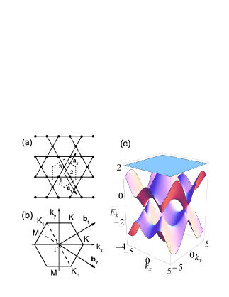
Figure 1: (color online) (a) Lattice structure of the Kagom$\acute{e}$ lattice. The region enclosed by the dash lines represents the Wigner-Seitz unit cell. $\mathbf{a}_{1}$ and $\mathbf{a}_{2}$ are the lattice unit vectors. The lattice sites in each unit cell are labeled by 1, 2, and 3. (b) The first Brillouin zone. $\mathbf{b}_{1}$ and $\mathbf{b}_{2}$ are the reciprocal-lattice vectors. (c) The electronic dispersion for $t_{12}=t_{23}=t_{31}=1.0$. The Dirac cones are located at $K$($K_{1}$) and $K^{\prime}$($K^{\prime}_{1}$) points as labeled in Fig.(b).

We start from the tight-binding model on a 2D metallic Kagom$\acute{e}$ lattice,

$$\hat{H}=-\sum_{\langle ij\rangle,\sigma}(t_{ij}\hat{c}^{{\dagger}}_{i\sigma}\hat{c}_{j\sigma}+\mathrm{H}.\mathrm{C}.),$$ (1)

where $\hat{c}_{i\sigma}$($\hat{c}^{{\dagger}}_{i\sigma}$) annihilates(creates) an electron with spin $\sigma$($\sigma=\uparrow,\downarrow$) on site $i$ and $t_{ij}$ is the hopping integral between the nearest neighbors. Considering that there are three sites in each unit cell [see Fig. 1(a)], we can write Eq.( 1) in the momentum space as $\hat{H}=\sum_{\mathbf{k}\sigma}\hat{\Psi}^{{\dagger}}_{\mathbf{k}\sigma}M(\mathbf{k})\hat{\Psi}_{\mathbf{k}\sigma}$. Where $\hat{\Psi}_{\sigma}(\mathbf{k})=(\hat{c}_{\mathbf{k}1\sigma},\hat{c}_{\mathbf{k}2\sigma},\hat{c}_{\mathbf{k}3\sigma})$, and $M(\mathbf{k})$ is a $3\times 3$ matrix

$$M(\mathbf{k})=\left(\begin{array}[]{ccc}0&\varepsilon_{12}(\mathbf{k})&\varepsilon_{13}(\mathbf{k})\\ \varepsilon_{21}(\mathbf{k})&0&\varepsilon_{23}(\mathbf{k})\\ \varepsilon_{31}(\mathbf{k})&\varepsilon_{32}(\mathbf{k})&0\end{array}\right),$$ (5)

with $\varepsilon_{12}(\mathbf{k})=\varepsilon_{21}(\mathbf{k})=-2t_{12}\cos(\mathbf{k}\cdot\mathbf{\delta}_{1})$, $\varepsilon_{13}(\mathbf{k})=\varepsilon_{31}(\mathbf{k})=-2t_{31}\cos(\mathbf{k}\cdot\mathbf{\delta}_{3})$ and $\varepsilon_{23}(\mathbf{k})=\varepsilon_{32}(\mathbf{k})=-2t_{23}\cos(\mathbf{k}\cdot\mathbf{\delta}_{2})$. $\mathbf{\delta}_{1}$, $\mathbf{\delta}_{2}$ and $\mathbf{\delta}_{3}$ are the nearest-neighbor vectors, $\mathbf{\delta}_{1}=(1/2)\hat{x}$, $\mathbf{\delta}_{2}=(1/4)\hat{x}+(\sqrt{3}/4)\hat{y}$, $\mathbf{\delta}_{3}=-(1/4)\hat{x}+(\sqrt{3}/4)\hat{y}$. For the isotropic case ($t_{12}=t_{23}=t_{31}=t$), the energy bands are,

$$E_{\pm}(\mathbf{k})=-t\pm t\sqrt{1+f(\mathbf{k})},\ \ E_{3}(\mathbf{k})=2t,$$ (6)

where $f(\mathbf{k})=8\cos(k_{x}/2)\cos(k_{x}/4+\sqrt{3}k_{y}/4)\cos(k_{x}/4-\sqrt{3}k_{y}/4)$, and the energy band structure is shown in Fig. 1(c). The two dispersive bands $E^{+}$ and $E^{-}$ contact at the Dirac point $K=(4\pi/3,0)$[or $K^{\prime}=(2\pi/3,2\pi/\sqrt{3})$]. Near the Dirac point $\mathbf{q}=\mathbf{k}-\mathbf{K}$, the electrons behave as Dirac fermions with the approximated dispersion,

$$E_{\pm}=-t\pm v_{F}|\mathbf{q}|+O[(q/K)^{2}],$$ (7)

$v_{F}=3\sqrt{2}t/4$ is the Fermi velocity. Thus, except for an additional flat band $E_{3}$, the two dispersive energy bands are similar to those in graphene. As a result, an unconventional QHE as that found in graphene is expected on the isotropic Kagom$\acute{e}$ lattice around the Fermi level $\mu=-t$ (corresponding to the electron filling $1/3$).

In an uniform magnetic field applied perpendicular to the sample plane, the tight-binding Hamiltonian is,

$$\hat{H}=-\sum_{\langle ij\rangle,\sigma}(t_{ij}e^{i\alpha_{ij}}\hat{c}^{{\dagger}}_{i\sigma}\hat{c}_{j\sigma}+\mathrm{H}.\mathrm{C}.).$$ (8)

The Hamiltonian Eq.(5) will be diagonalized numerically on a finite lattice with size $N=3\times L_{1}\times L_{2}$(factor three counts the three sites in each unit cell). The magnetic flux per triangular is chosen to be $\phi=\sum_{\triangle}\alpha_{ij}=\frac{2\pi}{M}$, with $M$ an integer, then the total flux $\Phi=\frac{16\pi N}{3M}$ through the lattice is taken to be an integer to satisfy the periodic boundary condition. Typically, $N=3\times 320\times 320$ and $\phi=\frac{2\pi}{2560}$ are used in numerical calculations. After the diagonalization, the Hall conductivity $\sigma_{xy}$ is calculated with the Kubo formula

$$\sigma_{xy}=A\sum_{\varepsilon_{\alpha}<E_{F}}\sum_{\varepsilon_{\beta}>E_{F}}\frac{\langle\alpha|v_{x}|\beta\rangle\langle\beta|v_{y}|\alpha\rangle-\langle\alpha|v_{y}|\beta\rangle\langle\beta|v_{x}|\alpha\rangle}{(\varepsilon_{\alpha}-\varepsilon_{\beta})^{2}},$$ (9)

where $A=i2e^{2}/S\hbar$ with $S$ the area of the system, $v$ is the velocity, $\varepsilon_{\alpha}$ and $\varepsilon_{\beta}$ are the corresponding eigenvalues of the eigenstates $|\alpha\rangle$ and $|\beta\rangle$. In the following, the hopping integrals $t_{12}=t_{31}=1.0$ are used as the energy unit and $t_{23}$ to acount for the anisotropy.

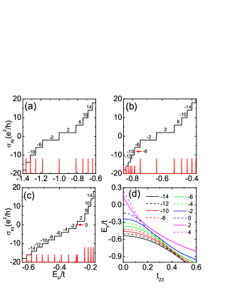
Figure 2: (color online) (a)-(c) Hall conductivities for different $t_{23}$ as a function of the Fermi energy and the corresponding density of states which is denoted by red vertical lines [(a) $t_{23}=1.0$. (b) $t_{23}=0.4$. (c) $t_{23}=0.15$]. The numbers on each plateau denote $\nu$ in $\sigma_{xy}=\nu e^{2}/h$. The red arrows in (b) and (c) indicate the transition point from $g_{s}=4$ to $g_{s}=2$. (d) Phase diagram showing the gradual splitting of the Hall plateaus with the decrease of $t_{23}$. The solid lines denote the original plateaus and the dashed lines the new plateaus induced by the anisotropy.

In Fig. 2, the Hall conductivity $\sigma_{xy}=\nu\frac{e^{2}}{h}$ and the electron density of states(DOS) are plotted for the different $t_{23}$. For the isotropic case with $t_{23}=1.0$, the Hall plateaus satisfy the unconventional quantization rule $\nu=(n+1/2)g_{s}$ with a degeneracy factor $g_{s}=4$ for each Landau level(LL) to count two spin components and two Dirac points. The $1/2$ shift of the Hall plateaus is due to a nonzero Berry phase at the Dirac points Mikitik , or can be simply explained as arising from the existence of a zero mode as seen from the DOS shown in Fig.2(a). This numerical result is consistent with the above analytical calculation, showing that the QHE on the isotropic Kagom$\acute{e}$ lattice exhibits the same behavior as that in graphene.

Decreasing $t_{23}$ to introduce the anisotropy in the hopping integral, one will find that the steps in Hall conductivity split at the mid-point gradually, as shown in Fig.2(b) and Fig.2(c). Concomitant with the splitting, a new Hall plateau emerges between every two Hall plateaus and the degeneracy factor $g_{s}$ changes from $4$ to $2$. Basically, one may expect that, upon the introduction of the anisotropy, the rotational symmetry of the isotropic Kagom$\acute{e}$ lattice will be broken, and consequently the degenerate energy levels will be separated. Indeed, at the energy levels where the step splitting in Hall conductivity occurs, the peak of DOS (denoted as red vertical lines in Fig.2) is split into two adjacent peaks with half a previous height. However, two nontrivial characters exhibit here. One is that the splitting does not happen as a whole simultaneously, but gradually from low energies to high energies with the decrease of $t_{23}$ (corresponding to the enhancement of the anisotropy). Moreover, whenever a splitting occurs, a new Hall plateau emerges. But, the next splitting does not happen in succession with the further decrease of $t_{23}$, instead the emerging plateau will grow firstly until it satisfies the new quantization rules for the Landau Level which will be addressed in the following. This process can also be clearly seen from the peak splitting in DOS. In this way, the QHE on the anisotropic Kagom$\acute{e}$ lattice exhibits a sequent quantum phase transition from low to high energies, as shown in the phase diagram presented in Fig.2(d). Secondly, in the case of $t_{23}>1$ (see Fig. 3(a)), the peaks in DOS does not split at any energy level in the reasonable parameter regime. As a result, at least for the largest anisotropy $t_{23}=2$ considered here, the QHE shows the same behavior to the isotropic case.

The quantum phase transition demonstrated above is in stark contrast to that on the honeycomb lattice(graphene) Sato ; Hasegawa ; Dietl ; Kohmoto , where the unconventional QHE changes into the conventional QHE with $\sigma_{xy}=2ne^{2}/h$ in the strong $t_{23}$ ($t_{23}>1$) regime, while no phase transition occurs for the weak $t_{23}$ ($t_{23}<1$) regime. In addition, the phase transition on the anisotropic honeycomb lattice occurs symmetrically starting from both the low and high energies, and gradually approaches to the zero-energy level, so that it exhibits a particle-hole symmetry.

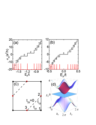
Figure 3: (color online) (a) and (b) are the Hall conductivity together with the DOS for $t_{23}=1$ and $t_{23}=0$, respectively. (c) The square lattice which is equivalent topologically to the Kagom$\acute{e}$ lattice for $t_{23}=0$. (d) The energy bands for the lattice in (c).

Next, let us study the character manifested by the new phase emerging in the quantum phase transition. This is accessible easily in the limit $t_{23}=0$, where the Kagom$\acute{e}$ lattice is topologically equivalent to the lattice in Fig. 3(c) with only the nearest neighbor hoppings. The three energy bands on this lattice can be found as, $E_{\pm}=\pm 2t\sqrt{\cos^{2}(k_{x}/2)+\cos^{2}(k_{y}/2)}$ and $E_{3}=0$, as shown in Fig. 3(d). Around $\mathbf{K}_{0}=(\pi,\pi)$, the bands $E_{\pm}$ have the linear dispersion $E_{\pm}(\mathbf{q})=\pm v_{F}|\mathbf{q}|$ with $v_{F}=\sqrt{2}t$. Because the flat band $E_{3}$ crosses the $\mathbf{K}_{0}$ point, the electrons do not behave as massless Dirac fermions. In this respect, the Hall conductivity shows a conventional behavior $\sigma_{xy}=2ne^{2}/h$. However, the energy of the LL follows a new quantization rule(Fig.3(b)). This can be obtained analytically by solving the low-energy Hamiltonian of the system, as given by

$$\hat{H}=\frac{v_{F}}{\sqrt{2}}\left(\begin{array}[]{ccc}0&\hat{p}_{x}&\hat{p}_{y}\\ \hat{p}_{x}^{{\dagger}}&0&0\\ \hat{p}_{y}^{{\dagger}}&0&0\end{array}\right),$$ (13)

under a uniform magnetic field $\mathbf{B}$ by replacing the momentum operator $\hat{\mathbf{p}}$ by $\hat{\mathbf{p}}+e\mathbf{A}$ with $\mathbf{A}=B(-y,0)$. The result turns out to be,

$$E(n)=\pm v_{F}\sqrt{(n+1/2)\hbar Be},\ n=1,2,3,\cdots.$$ (14)

This kind of distribution of the LL leads to a corresponding distribution of the Hall plateaus, which is different from that in conventional semiconductors $(n+1/2)\hbar\omega_{c}$, graphenes $v_{F}\sqrt{2n\hbar Be}$ and bilayer graphenes$\sqrt{n(n-1)}\hbar\omega_{c}$.

To understand the property of the quantum phase transition demonstrated above, we show in Fig.4 the evolution of the energy band with the hopping integral $t_{23}$ along the high symmetrical directions. First, we point out that the unconventional QHE is found numerically to be limited to a finite energy range (not shown here), which is the region from $A$ to $A^{\prime}$ (points of the van Hove singularity) in the dispersions shown in Fig.4. Outside this region, the QHE will exhibit a conventional behavior in Hall conductivity. For $t_{23}<1$ [Fig.4(a)], the two Dirac points, which are at $K$ and $K^{\prime}$ points in the isotropic case, approach each other along the $K-K^{\prime}$ direction with the decrease of $t_{23}$. Interestingly, in this process, the energy band around the $A$ point is suppressed and lifted upwards gradually, while that around the $A^{\prime}$ point is not changed. As a result, the low energy part will be excluded out of the unconventional regime. Therefore, the conventional Hall conductivity emerges at these energy levels.

On the other hand, for $t_{23}>1$ [Fig.4(b)] the two Dirac points approach each other along the $K_{1}-\Gamma-K^{\prime}_{1}$ direction [see Fig.1(b) for illustration]. Different from the case of $t_{23}<1$, the energy band around $A$ now is shifted downwards with the increase of $t_{23}$, so that the energy region exhibiting the unconventional Hall conductivity is enlarged. Therefore, no quantum phase transition is observed in the energy region considered.

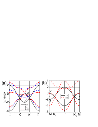
Figure 4: (color online) The energy bands for different $t_{23}$. (a) The energy bands for weak $t_{23}$ regime. Two typical energy bands are plotted along $\Gamma-K-K^{\prime}-\Gamma$ direction. The blue dash, and red dash-dot lines are corresponding to $t_{23}=0.4$ and $t_{23}=0.15$ respectively. (b) The energy bands for strong $t_{23}$ regime. The typical energy bands for $t_{23}=2$(the red dash lines) are plotted along $M-K_{1}-\Gamma-K_{2}-M^{\prime}$ direction. In the two figures, the black solid lines are the energy bands for the isotropic case($t_{23}=1$).

Finally, let us give a few comments on the possible experimental realization of the theoretical prediction elaborated here. The anisotropy of the hopping integral can be realized by the distortion of the lattice due to the monoclinic distortion, such as in $\mathrm{Cu_{(}3)V_{2}O_{7}(OH)_{2}\cdot 2H_{2}O}$ Bert , or by the difference in orbital characters on the atomic sites in each unit cell due to the Jahn-Teller effect, such as in $\mathrm{Cs_{2}Cu_{3}CeF_{12}}$ Amemiya . On the other hand, the Kagom$\acute{e}$ lattice has been proposed to be realized by implementing an optical lattice for ultra-cold atoms Santos ; Ruostekoski . In this regard, the ability to conveniently control the physical parameters in the system facilitates the realization of the anisotropy. It also worthwhile to point out that the 2D lattice in the limit $t_{23}=0$ as shown in Fig.3(c) is different from the Kagom$\acute{e}$ lattice, and may provide an interesting model system for experimental investigation on the special quantum dynamics demonstrated above.

In summary, we have study the quantum Hall effect on the anisotropic Kagom$\acute{e}$ lattice. The anisotropy is introduced by assuming one of the hopping integrals $t_{23}$ taking a different value. In the weak $t_{23}$ ($t_{23}<t_{12}$) regime, we find a new type of QHE characterized by the quantization rules for Hall conductivity $\sigma_{xy}=2ne^{2}/h$ and Landau Levels $E(n)=\pm v_{F}\sqrt{(n+1/2)\hbar Be}$, which is different from the known types. This phase evolves from the unconventional QHE with $\sigma_{xy}=4(n+1/2)e^{2}/h$ via a quantum phase transition, which occurs successively from low to high energies with the decrease of the hopping integral. This quantum phase transition is absent in the strong $t_{23}$ regime. Possible experimental realization of the theoretical prediction is also discussed.

- (1) R. E. Prange, S. M. Girvin, The Quantum Hall Effect(Springer, New York, 1990).
- (2) K. S. Novoselov, A. K. Geim, S. V. Morozov, D. Jiang, M. I. Katsnelson, I. V. Grigorieva, S. V. Dubonos, and A. A. Firsov, Nature(London) 438, 197 (2005).
- (3) Y. Zhang, Y. -W. Tan, H. L. Stormer, and P. Kim, Nature(London) 438, 201 (2005).
- (4) F. D. M. Haldane, Phys. Rev. Lett. 61, 2015 (1988).
- (5) Y. Zheng, and T. Ando, Phys. Rev. B 65, 245420 (2002).
- (6) V. P. Gusynin, and S. G. Sharapov, Phys. Rev. Lett. 95, 146801 (1999).
- (7) D. N. Sheng, L. Sheng, and Z. Y. Weng, Phys. Rev. B 73, 233406 (2006).
- (8) A. H. Castro Neto, F. Guinea, N. M. R. Peres, K. S. Novoselov and A. K. Geim, Rev. Mod. Phys. 81, 109 (2009).
- (9) K. S. Novoselov, E. Mccann, S. V. Morozov, V. I. Fal ko, M. I. Katsnelson, U. Zeitler, D. Jiang, F. Schedin, and A. K. Geim, Nat. Phys. 2, 177 (2006).
- (10) E. McCann and V. I. Fal ko, Phys. Rev. Lett. 96, 086805 (2006).
- (11) A. Mielke, J. Phys. A 24, L73 (1991).
- (12) M. Sato, D. Tobe, and M. Kohmoto, Phys. Rev. B 78, 235322 (2008).
- (13) Y. Hasegawa, R. Konno, H. Nakano, and M. Kohmoto, Phys. Rev. B 74, 033413 (2006).
- (14) P. Dietl, F. Pichon, and G. Montambaux, Phys. Rev. Lett. 100, 236405 (2008).
- (15) M. Kohmoto and Y. Hasegawa, Phys. Rev. B 76, 205402 (2007).
- (16) G. P. Mikitik and Yu. V. Sharlai, Phys. Rev. Lett. 82, 2147 (1999).
- (17) F. Bert, D. Bono, P. Mendels, F. Ladieu, F. Duc, J.-C. Trombe, and P. Millet, Phys. Rev. Lett. 95, 087203 (2005).
- (18) T. Amemiya, M. Yano, K. Morita, I. Umegaki, T. Ono, H. Tanaka, K. Fujii, and H. Uekusa, arXiv: 0906.1628 (2009).
- (19) L. Santos, M. A. Baranov, J. I. Cirac, H.-U. Everts, H. Fehrmann, and M. Lewenstein, Phys. Rev. Lett. 93, 030601 (1999).
- (20) J. Ruostekoski, arXiv: 0906.3042 (2009).