Critical exponents from cluster coefficients

Abstract

For a large class of repulsive interaction models, the Mayer cluster integrals can be transformed into a tridiagonal real symmetric matrix $R_{mn}$, whose elements converge to two constants. This allows for an effective extrapolation of the equation of state for these models. Due to a nearby (nonphysical) singularity on the negative real $z$ axis, standard methods (e.g. Padè approximants based on the cluster integrals expansion) fail to capture the behavior of these models near the ordering transition, and, in particular, do not detect the critical point. A recent work (Eisenberg and Baram, PNAS 104, 5755 (2007)) has shown that the critical exponents $\sigma$ and $\sigma^{\prime}$, characterizing the singularity of the density as a function of the activity, can be exactly calculated if the decay of the $R$ matrix elements to their asymptotic constant follows a $1/n^{2}$ law. Here we employ renormalization arguments to extend this result and analyze cases for which the asymptotic approach of the $R$ matrix elements towards their limiting value is of a more general form. The relevant asymptotic correction terms (in RG sense) are identified and we then provide a corrected exact formula for the critical exponents. We identify the limits of usage of the formula, and demonstrate one physical model which is beyond its range of validity. The new formula is validated numerically and then applied to analyze a number of concrete physical models.

I INTRODUCTION

It is often said that the mechanism underlying phase transitions is the decrease of internal energy in the ordered phase. However, it has been shown long ago that melting is dominated by the strong short ranged repulsive forces, and the related solid-fluid transitions are entropy-driven. Accordingly, purely repulsive models have been often used to study the fluid equation of state towards the structural ordering transition. The most striking demonstration of these observations is given by the family of hard-core models, which have long played a central role in this field. In these models, particles interact exclusively through an extended hard core, and there is no temperature scale associated with the potential (interaction energy is either infinite inside the exclusion region or zero outside). Thus, temperature and energy play no role, and the dynamics is completely determined by entropy considerations. Yet, these models exhibit various types of ordering transitions. They include, for example, the famous isotropic-nematic transition in a three dimensional system of thin hard rods onsager ; zwanzig , as well as the extensively studied hard spheres models wood ; alder ; alderdisks ; hoover ; michels , undergoing a first order fluid-solid transition for $d\geq 3$ and, presumably, a second order transition from a fluid to the hexatic phase hexatic1 ; hexatic2 . These models are purely entropy-driven, yet they capture the essential molecular mechanism that drives freezing transitions.

A complete description of the fluid phase is provided by the Mayer cluster series in terms of the activity, $z=\exp(\beta\mu)$, where $\mu$ is the chemical potential. For purely repulsive potentials, the radius of convergence of the cluster series is known to be determined by a singularity on the negative real axis, $z=-z_{0}$, typically very close to the origin Groeneveld . Near this point, the singular part of the density is characterized by the critical exponent $\sigma$:

$$\rho_{\rm sing}(z)\simeq(z+z_{0})^{\sigma}.$$

As a result of this singularity, the radius of convergence of the Mayer series includes only the extremely low density regime, and the fluid-solid transition is way beyond it. It is therefore desirable to find a way to extend the information contained in the cluster integrals series to provide information about the behavior of the system close to the ordering transition region. In particular, one is interested in the critical exponent $\sigma^{\prime}$ characterizing the density near the physical termination point of the fluid $z_{t}$:

$$\rho_{\rm sing}(z)\simeq(z-z_{t})^{\sigma^{\prime}}.$$

It has been shown that this goal may be achieved by transforming the cluster integral series into a tridiagonal symmetric matrix form baramr . The matrix elements $R_{nm}$ adopt a clear asymptotic form, and converge extremely fast to two different constants: $A$ (off-diagonal) and $B$ (diagonal). This fact can then be utilized to obtain good approximants for the fluid density far outside of the convergence circle of the power series baramf ; baramr2 ; eb06 . Like Padè methods, these approximants are consistent with the known elements to all available orders. However, the $R$ matrix scheme seems to fit much better purely repulsive systems, as it incorporates the existence of two singular points on the real axis baraml ; laifisher ; parkfisher . Yet, a major shortcoming of this approach was its failure at the critical regime. It is easy to prove (see below) that tridiagonal $R$ matrices described at the asymptote by two constant values lead to universal critical exponents $\sigma=\sigma^{\prime}=1/2$ at both singularities, which are obviously wrong. Thus, the above approach fails when one is in close vicinity to the transition region.

	N4	N5	Triangular N2
$n$	$nb_{n}$	$nb_{n}$	$nb_{n}$
1	1	1	1
2	-21	-25	-13
3	529	757	205
4	-14457	-24925	-3513
5	413916	860526	63116
6	-12213795	-30632263	-1169197
7	368115798	1114013874	22128177
8	-11270182473	-41160109013	-425493585
9	349244255338	1539411287905	8282214430
10	-10926999690716	-58134505912850	-162784518218
11	344563541226829	2212737992414500	3224828597398
12	-10935950490228951	-84773398978877767	-64304659129557
13	348996298644804045	3265709152114882760	1289359180917536
14	-11189659831729226400	-126396751968240912540	-25974798852799663
15	360221541077745515049	4911995555642255534862	525411435083794040
16	-11637415720384495480425	-191566536035975787182277	-10665744051246882913
17	377133138423022266192030	7494404630272576450625728	217191426304757630038
18	-12255532866263525229229458	-294007038999894901106531809

Table 1: Mayer cluster coefficients $nb_{n}$ for various models

A partial solution for this problem was recently found, noticing that for many of the studied models not only the matrix element approach a constant but also the asymptotic correction to the constant takes a universal form, following a $1/n^{2}$ decay of the elements to their constant asymptotic value eli :

$$B_{n}\equiv R_{n,n} = B+b/n^{2}$$

$$A_{n+1/2}\equiv R_{n,n+1} = A+a/(n+1/2)^{2}.$$ (1)

Under these circumstances, one is able to analytically calculate the critical exponents at both fluid termination point (the physical one, at the ordering transition or at the termination of the super-cooled fluid, and the nonphysical one on the negative real z-axis). These exponents depend on the amplitudes of the $1/n^{2}$ corrections, and generally deviate from $1/2$. This approach works satisfactorily for many models and tests well against the known result for the nonphysical singularity that predicts universal critical exponents depending on dimensionality alone.

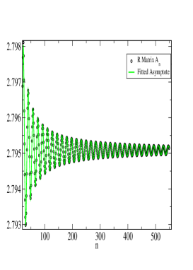
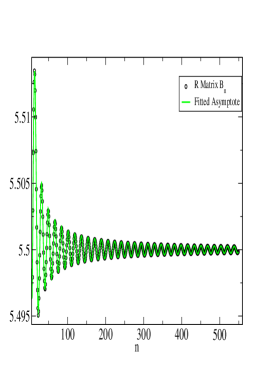
Figure 1: Hard hexagons matrix elements, fitted to the form (2), with $A=\sqrt{125}/4$ $a=0.0027$ $a^{\prime}=-0.063$ $B=5.5$ $b=0.627$ $b^{\prime}=0.129$ $q=0.36$

Yet, while many models indeed show this simple $1/n^{2}$ decay, we have found out that some other models exhibit different asymptotic behavior. For example, the $R$ matrix elements of the hard hexagons model baxter are presented in fig 1. As this is an exactly solvable model, one is able to produce a large number of cluster integrals. Doing so, we note that while the first few elements seem to follow the $1/n^{2}$ rule, the asymptotic behavior is quite different. The matrix elements do converge to two constants as expected, but their leading asymptotic behavior follows an oscillatory $1/n$ decay rather than the above mentioned $1/n^{2}$. This finding raises the question of how to deal with $R$ matrices whose correction deviates from the (1) form. Moreover, it sheds doubt on the applicability of former results to other models where only a few cluster integrals are known: one may argue that the hard hexagons example shows that the $1/n^{2}$ behavior is only a transient one, and the true asymptotics of all these models is different. Indeed, extension of the available series to higher coefficients of the Mayer expansion allowed us to see in a number of additional models that the seeming $1/n^{2}$ behavior is accompanied by additional corrections, including an oscillatory $\cos(qn)/n$ term that becomes dominant in the asymptote. We observed such oscillations, for example, for hard-core two-dimensional square lattice gas with exclusion shell up to second (N2 model), third (N3 model) and fourth (N4 model) nearest neighbors.

As this oscillatory term dominates for large $n$, the validity of the results of eli is put in question. Therefore, we set out to study the effect of this additional correction term on the critical behavior of the equation of state. Here we extend the previous result and explore the case of matrix elements taking the asymptotic form

$$R_{n,n} = B+\frac{b}{n^{2}}+b^{\prime}\frac{\cos(qn)}{n}$$

$$R_{n,n+1} = A+\frac{a}{(n+1/2)^{2}}+a^{\prime}\frac{\cos[q(n+1/2)]}{n+1/2}$$ (2)

Using an analytical RG-like decimation scheme, we show that in this case the critical exponents are given by

$$\sigma=\frac{1}{2}\sqrt{1-\frac{4(2a+b)}{A}-\frac{[2a^{\prime}\cos(q/2)+b^{\prime}]^{2}}{[1-\cos(q)]A^{2}}}$$

$$\sigma^{\prime}=\frac{1}{2}\sqrt{1-\frac{4(2a-b)}{A}-\frac{[2a^{\prime}\cos(q/2)-b^{\prime}]^{2}}{[1-\cos(q)]A^{2}}}$$ (3)

thus generalizing the results of eli . We also discuss the possible effect of other kinds of corrections, and conclude that they do not affect the critical exponent as long as the spectrum of the matrix remains intact. We verify the result by extensive numerical study of artificial models and by analysis of the exactly solvable hard-hexagons model. The next-nearest neighbor exclusion model on a triangular lattice is discussed as an example in which the spectrum does not remain intact and our approach breaks down. Finally, we apply our formula to the two models that have been recently studied by means of Monte-Carlo (MC) simulations levin : the hard-core two-dimensional square lattice gas with exclusion shell up to fourth (N4 model) and fifth (N5 model) nearest neighbors.

II Analysis

For the sake of completeness, we start with a brief review of the approach presented in eli . The Mayer cluster integrals provide a low-$z$ expansion for the density of a fluid:

$$\rho(z)=\sum\limits_{n=1}^{\infty}nb_{n}z^{n},$$ (4)

where $b_{n}$ is the $n^{\rm th}$ Mayer cluster integral. It is always possible (see appendix A for an explicit construction) to define a tridiagonal symmetric $R$ matrix which satisfies the condition ($n\geq 1$)

$$(R^{n})_{11}=(-1)^{n}(n+1)b_{n+1}.$$ (5)

The density may then be expressed in terms of $R$:

$$\rho(z)=\sum\limits_{n=1}^{\infty}{nb_{n}z^{n}=\sum\limits_{n=0}^{\infty}{({-1})^{n}z^{n+1}({R^{n}})_{11}=z({I+zR})_{11}^{-1}}}.$$ (6)

Alternatively, the matrix inversion in the previous equation may be expressed in terms of the spectrum $\lambda$ of the $R$ matrix, and the corresponding eigenvectors $\psi(\lambda)$:

$$\rho(z)=\sum\limits_{\lambda}\frac{\psi_{1}(\lambda)^{2}}{z^{-1}+\lambda},$$ (7)

where $\psi_{1}(\lambda)$ is the first component of the $\psi(\lambda)$ vector.

The reciprocals of the eigenvalues of this matrix are the Yang-Lee zeroes of the grand-canonical partition function. For all purely repulsive models studied to date, the R matrices are real-valued, and thus their eigenvalues are also real ($R$ is symmetric by construction). There is yet no proof that this is indeed the case for all such models, but construction of $R$ matrices for dozens of different lattice and continuum purely repulsive models (see, e.g., eb06 ; baraml ; eli and this work) provides strong evidence for it: in all cases studied the matrix elements were real to all orders calculated. Furthermore, as mentioned above, the matrix elements in all models studied adopt a clear asymptotic pattern, converging quickly to a (real) constant. Therefore the possibility that some higher order element may become complex seems improbable.

For these real $R$ matrices the spectrum of the matrix lies on the real axis in an interval $(-z_{t}^{-1},z_{0}^{-1})$ (and the Yang-Lee zeroes lie on two intervals along the real activity axis: $z<-z_{0}$ and $z>z_{t}$). It follows from (7) that the density $\rho(z)$ has two singular points at $z$ values for which $-z^{-1}$ coincides with the spectrum edges of the $R$ matrix, leading to vanishing of the denominator on the right-hand side. The critical behavior of the density $\rho(z)$ near the physical and non-physical singularities is therefore determined by the structure of the residue $\psi_{1}(\lambda)$ at the spectrum edges.

For example, we look at a matrix with two constants along the three main diagonals, $B$ (diagonal) and $A$ (off-diagonal). The eigenvalues are $\lambda(k)=B+2A\cos(k)\,\,\,\,(0<k<\pi)$ and the eigenvectors are $\psi_{n}[\lambda(k)]=\sin(nk)$. The critical points are then

$$-z_{0}^{-1}=-(B+2A)$$

(corresponding to $k=0$), and

$$z_{t}^{-1}=2A-B$$

($k=\pi$), where $\psi_{1}(k)\equiv\psi_{1}[\lambda(k)]\sim k$ and $\psi_{1}(k)\equiv\psi_{1}[\lambda(k)]\sim(k-\pi)$ respectively. Expanding the integral in (7) for $z\sim-z_{0}$ and $z\sim z_{t}$ one finds that the density terminates at both ends with a square-root singularity.

We now consider a general $R$ matrix taking the form

$$B_{n}\equiv R_{n,n} = B+\delta B_{n}$$

$$A_{n+1/2}\equiv R_{n,n+1} = A+\delta A_{n+1/2}.$$ (8)

The critical behavior is determined by the long-wavelength, slowly-varying, eigenvectors and therefore the eigenvalue equation (we treat the nonphysical critical point only, analysis of physical point is essentially identical)

$$A_{n-1/2}\psi_{n-1}+B_{n}\psi_{n}+A_{n+1/2}\psi_{n+1}=\lambda\psi_{n}$$ (9)

may be studied in the continuum limit, taking the form of a differential equation in the variable $x=kn$. For the general case (8), the discrete equations (9) transform into

$$f^{\prime\prime}(x)+f(x)+\frac{[\delta B_{n}+\delta A_{n-1/2}+\delta A_{n+1/2}]n^{2}}{Ax^{2}}f(x)=0.$$ (10)

As long as the corrections $\delta B$ and $\delta A$ are small enough (see below) the spectrum does not change. The eigenvectors, nevertheless, are modified. In eli the $R$ matrix was assumed to take the form (1), and then the differential equation (10) is reduced into a Bessel equation. A closed form for the eigenvectors is available, and one obtains the critical behavior of the density near the two branch points $\rho(z_{c})-\rho(z)=(z_{c}-z)^{\sigma}$ (or $\rho(z)=(z_{c}-z)^{-\sigma}$ if the density diverges at criticality, such as the case of the non-physical singularity in $d\leq 2$). The critical exponents are given by

$$\sigma=\frac{1}{2}\sqrt{1-4\frac{{2a-b}}{A}},\,\,\,\,\,\,\,\,\sigma^{\prime}=\frac{1}{2}\sqrt{1-4\frac{{2a+b}}{A}}$$ (11)

where $\sigma(\sigma^{\prime})$ is the exponent of the non-physical (physical) branch point.

This approach, however, cannot be extended straight-forwardly to study a general correction to the matrix elements: while for $1/n^{2}$ corrections (10) can be written in terms of $x=kn$ alone, independently of $k$, a general correction term results in a $k$-dependent differential equation. More importantly, considering terms $O(1/n^{3})$ in the differential equation approach leads to an essential singularity at the origin, resulting in transition layer solutions and complicated behavior at the origin. These terms indeed show up when one analyzes real $R$ matrices (see below for the N4 and N5 models). Third, the mapping to a differential equation relies on the slow variation of the eigenvectors and is bound to fail for correction terms of the form (2) that induce an intrinsic “length”-scale (on the $n$ axis) into the problem.

We thus present here a complementary approach to study the general correction term, which is based on the idea of renormalization. In their discrete form, the eigenvalue equations (9) form an infinite linear system of equations. Since the system is tridiagonal, it is quite easy to eliminate half of the variables, e.g. all variables $\psi_{n}$ for $n$ even. This effectively removes half of the rows and half of the columns in the matrix, “tracing out” half of the degrees of freedom in the problem. One obtains a new tridiagonal system of equations, or a renormalized $R$ matrix, with the same eigenvalues and new vectors $\tilde{\psi}(k)$ that are simply related to the former ones $\tilde{\psi}_{n}(k)=\psi_{2n-1}(k)$. In particular, $\tilde{\psi}_{1}(k)=\psi_{1}(k)$. The density as a function of $z$ is fully determined by the spectrum and $\psi_{1}(\lambda)$ through (7). Thus, the renormalized $R$ matrix may be utilized to generate the same equation of state and the same critical behavior as the original one. Explicitly, the reduced eigenvalue equation after one such decimation process takes the form (n odd; $A_{n+1/2}=B_{n}=0$ for $n\leq 0$)

$$\frac{A_{n-3/2}A_{n-1/2}}{\lambda-B_{n-1}}\psi_{n-2}+(\frac{A_{n-1/2}^{2}}{\lambda-B_{n-1}}+\frac{A_{n+1/2}^{2}}{\lambda-B_{n+1}}+B_{n})\psi_{n}+\frac{A_{n+1/2}A_{n+3/2}}{\lambda-B_{n+1}}\psi_{n+2}=\lambda\psi_{n}.$$ (12)

Accordingly, the $R$ matrix elements transform, under such decimation, according to

$$B_{n}^{\prime} = \frac{A_{2n-3/2}^{2}}{\lambda-B_{2n-2}}+\frac{A_{2n-1/2}^{2}}{\lambda-B_{2n}}+B_{2n-1}$$ (13)

$$A_{n+1/2}^{\prime} = \frac{A_{2n-1/2}A_{2n+1/2}}{\lambda-B_{2n}}.$$ (14)

In the transformed linear system $\tilde{\psi}_{n}$ is in fact $\psi_{2n-1}$, so for a given functional form for $A_{n}$ and $B_{n}$ one should change variables $n^{\prime}\to 2n-1$. Note that the renormalization transformation is $\lambda$-dependent. Since the density in the vicinity of the critical points is determined by the spectrum edges only, this poses no difficulty.

As a first demonstration of this RG scheme, one may look at the solvable case of $1/n^{2}$ correction. Substituting $A_{n}=A+a/n^{2}$, $B_{n}=B+b/n^{2}$ and $\lambda=2A+B$ into (12), one obtains

$$A_{n+1/2} \to A/2+\frac{1}{8n^{2}}(4a+b)+O(\frac{1}{n^{3}})$$ (15)

$$B_{n} \to (A+B)+\frac{1}{n^{2}}(a/2+3b/8)+O(\frac{1}{n^{3}}).$$

Clearly, the spectrum edge, defined by the asymptotic value of $A_{n-1/2}+A_{n+1/2}+B_{n}$ to be $-z_{0}=-(2A+B)^{-1}$ is conserved under the decimation. Moreover, the correction term $(\delta A_{n-1/2}+\delta A_{n+1/2}+\delta B_{n})/A$ which appears in the differential equation and determines the critical exponent by (11), is also stable under the transformation and remains equal to $(2a+b)/An^{2}$, as expected.

Applying the same transformation for corrections of the form $1/n^{\alpha}$ i.e. $A_{n}=A+a^{\prime\prime}/n^{\alpha}$,$B_{n}=B+b^{\prime\prime}/n^{\alpha}$, results in

$$\frac{1}{A}(\delta A_{n-1/2}+\delta A_{n+1/2}+\delta B_{n})\to\frac{1}{2^{\alpha-2}}\frac{2a^{\prime\prime}+b^{\prime\prime}}{A}\frac{1}{n^{\alpha}}.$$ (16)

Therefore, one may conclude that for $\alpha>2$ the correction term in the differential equation (10) is suppressed by successive applications of the RG decimation transformations. Therefore, these correction terms are irrelevant in determining the critical exponents.

We now employ the RG scheme to study the case of main interest: $1/n$-modulated oscillations, as observed for the hard hexagons model

$$A_{n+1/2} = A+a^{\prime}\cos[q(n+1/2)]/(n+1/2)$$

$$B_{n} = B+b^{\prime}\cos(qn)/n.$$ (17)

The transformation of the differential equation correction term $(\delta A_{n-1/2}+\delta A_{n+1/2}+\delta B_{n})/A$ upon one decimation step is given by

$$\frac{1}{A}(\delta A_{n-1/2}+\delta A_{n+1/2}+\delta B_{n}) = \frac{2a^{\prime}\cos(q/2)+b^{\prime}}{A}$$

$$\to\frac{[2a^{\prime}\cos(q/2)+b^{\prime}][1+\cos(q)]\cos(2qn)}{An} + \frac{[2a^{\prime}\cos(q/2)+b^{\prime}]^{2}}{2A^{2}}\frac{1}{n^{2}}+O(\cos(2q)/n^{2},1/n^{3})$$ (18)

Obviously, the real-space renormalization process induces a change in the frequencies $q\to 2q$. In addition, (i) the $\cos(qn)/n$ term is multiplied by a factor of $[1+\cos(q)]$, and three more terms emerge: (ii) a new $1/n^{2}$ term, (iii) terms $O(\cos(2qn)/n^{2})$ and (iv) terms $O(1/n^{3})$. Iterating this procedure $N$ times, one obtains from (i) $(2a+b)\to(2a^{\prime}+b^{\prime})\prod\limits_{n=1}^{N}[1+\cos(2^{n-1}q)]$. The newly emerging $1/n^{2}$ terms (ii) combine to take the form $\frac{(2a^{\prime}+b^{\prime})^{2}}{16A}\sum\limits_{n=0}^{N}\prod\limits_{m=1}^{n}[1+\cos(2^{m-1}q)]^{2}$. The first term gets exponentially small for large $N$: $\prod\limits_{n=1}^{N}[1+\cos(2^{n-1}q)]\simeq 4^{-N}$ (see Appendix B), and thus could be neglected. The sum over the products in the second term converges to $[1-\cos(q)]^{-1}$ (see Appendix B). This second term does affects the critical behavior as it adds up to the $1/n^{2}$ terms in the $R$ matrix. The $1/n^{3}$ terms (iii) may be neglected as their amplitude decreases: each existing $1/n^{3}$ term decreases by factor $2$ upon an RG step, according to (16). While a new term is being added from the transformation (12), the sum of all contributions still decreases exponentially with the number $N$of RG steps. The $\cos(qn)/n^{2}$ terms (iv) transform under decimation in an analogous way to the original $\cos(qn)/n$ term: they get multiplied by a factor $1+\cos(q)$ resulting in an exponential decay, and give rise to new $O(1/n^{4})$ terms (analogous to the $O(1/n^{2})$ terms generated from decimation of the $\cos(qn)/n$), as well as faster decreasing terms. Again, the $1/n^{4}$ exponentially decrease through decimation by (16) and are therefore neglected. In summary, the net effect of the $\cos(qn)/n$ term after a large number of RG steps is the creation of a new $1/n^{2}$ term. These terms, emerging from the decimation process, can then be analyzed using the mapping to the Bessel differential equation as described in eli .

Up to this point we treated the pure $\cos(qn)/n$ case. Similar analysis may be done for the mixed case, where both $\cos(qn)/n$ and $1/n^{2}$ terms are present (as happens for the physical models to be discussed). It turns out that the transformation equation (12) does mix the correction terms, as the numerator of $(A_{n}A_{m})/(\lambda-B_{l})$ is quadratic in the off-diagonal elements. However, the mixed terms will follow the form $\cos(qn)/n^{3}$ which can be ignored based on arguments similar to those presented above for the $\cos(qn)/n^{2}$ terms. Multiplicative cross-terms could be relevant (in RG sense) only if they decay $O(1/n^{2})$ or slower. Thus, one may simply add the original $1/n^{2}$ terms to those emerging from RG. Collecting the $O(1/n^{2})$ terms originating from both the functional form of the matrix elements and the decimation process for oscillatory terms, one obtains the closed form (I) for the critical exponents in the general case (having both $\cos(qn)/n$ terms and $1/n^{2}$ terms).

We note that the critical exponents in (I) do not depend on $B$. This can be readily understood looking at equation (7). A change in $B$ results in a constant addition to the whole spectrum of $R$, without modifying its eigenvectors. Looking at the expression (7) for the density, it becomes clear that the effect of a constant added to the eigenvalues of $R$ on the density is equivalent to a constant shift in $z^{-1}$. That is, if the density of the $B=0$ matrix is $\rho_{0}(z)$, the density for finite $B$, $\rho(z;B)$, is simply

$$\rho(z;B)=\rho_{0}(\frac{1}{z^{-1}+B}).$$

Therefore, the value of $B$ affects the location of the critical points, but do not change the critical exponents.

Finally, we note that if the amplitude of the correction to a constant matrix is strong enough, one obtains from (I) an imaginary value for $\sigma$. When this happens, both solutions of the differential equation (10) diverge at the origin bessel . Consequently, there are no solutions to the eigenvalue problem (9) for $k\sim 0$, or $\lambda\sim 2A+B$. In other words, a perturbation of the constant matrix which is strong enough to make $\sigma$ imaginary modifies the spectrum of the matrix, such that the spectrum edge shifts from $2A+B$. In these cases the critical point is not given by $-z_{0}=-(2A+B)^{-1}$. Similarly, whenever $\sigma^{\prime}$ becomes imaginary, the physical singularity shifts from $z_{t}=(2A-B)^{-1}$. In both cases, the corresponding critical exponents are not given by (I). This scenario is realized for the next-nearest neighbor exclusion model on the triangular lattice (see below).

III Numerical Study

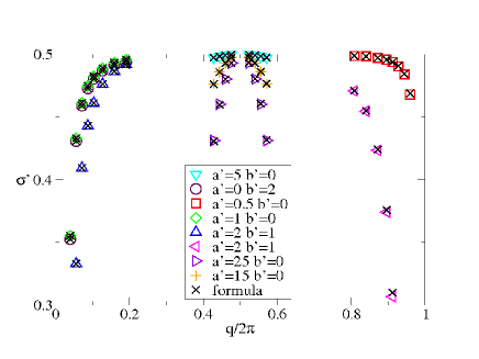
Figure 2: Critical exponents as measured from equation of state (19), compared with the exact prediction (I) for various choices of $\cos(qn)/n$ corrections.

In order to test our results, we have constructed various tridiagonal symmetric $R$ matrices with prescribed matrix-elements asymptotic form, and compared the prediction (I) with the critical behavior as measured from the equations of state calculated by (6) for these models. First, we looked at matrices obeying (17), with the parameters $A=16$ and $B=31$ ($z_{t}=1$), and various combinations of $a^{\prime}$,$b^{\prime}$ and $q$. We have also modified $A$ while keeping the other parameters fixed to check the $A$ dependence. For these $R$ matrices, one is able to consider as many coefficients as desired. Thus, the size of the sub-matrices studied is considerable, and the matrix inversion of (6) is costly. Instead, the density $\rho$ can be equivalently calculated using the continued fraction representation

$$\rho(z)=\cfrac{1}{R_{1,1}+1/z-R_{1,2}^{2}\cfrac{1}{R_{2,2}+1/z-R_{2,3}^{2}\cfrac{1}{R_{3,3}+1/z-R_{3,4}^{2}\cdots}}}$$ (19)

which typically converges rather quickly (except for the immediate vicinity of the transition point). Figure  2 compares the critical exponent $\sigma^{\prime}$ obtained by fitting the density as given by (19) for $z$ close to the termination point $z_{t}$ with the theoretical prediction of (I). The results are in excellent agreement, except for a few points where the numerical calculation of the density was difficult due to slow convergence of the continued fraction in the immediate vicinity of the critical point. We also calculated the density for $R$ matrices with both $1/n^{2}$ and $\cos(n)/n$ corrections, i.e. following (2). The agreement between the theoretical prediction of (I) and the measured critical exponent was again excellent. Another special case we checked was that of a $1/n^{3}$ correction. This is the most dominant correction for which we predict no change to the critical exponent of the const matrix. Using the same constants $A$ and $B$, we looked at correction amplitudes up to $a^{\prime\prime}=30$, and verified that the critical exponent indeed does not change: $\sigma^{\prime}=0.5$ as expected.

	N4		N5		Triangular N2
$n$	$B_{n}$	$A_{n}$	$B_{n}$	$A_{n}$	$B_{n}$	$A_{n}$
1	21	9.3808315196	25	11.489125293	13	6
2	17.045454545	8.7248457800	20.454545455	10.570731201	10.555555556	5.5674871873
3	17.024781724	8.6098449927	20.518434015	10.405877593	10.550189740	5.4798922624
4	17.018848337	8.5688057487	20.535452306	10.348827163	10.576974307	5.4386602176
5	17.017061106	8.5493273256	20.540912637	10.322722326	10.600981921	5.4160504788
6	17.016534640	8.5385152615	20.543142266	10.308577639	10.615727211	5.4037594351
7	17.016426427	8.5318795598	20.544349327	10.299999108	10.622716309	5.3973336220
8	17.016464632	8.5275092336	20.545165481	10.294371298	10.625196191	5.3938592930
9	17.016552228		20.545790085

Table 2: R matrix elements for various models

IV Applications to physical models

Analysis of the R matrix as detailed above may be used to predict the critical behavior of all models with purely repulsive interactions. Our results apply equally to continuum and lattice models in all dimensions. Here we demonstrate applications to a number of 2D hard-core lattice gas models.

For all the models to follow, we have calculated the cluster integrals to a high order (in order to calculate the $R$ matrix). It is natural to compare standard series analysis methods guttmann to the results to be obtained from the $R$-matrix. We have applied the ratio method, Dlog Padè and differential approximants to the models to follow. In general, ratio analysis of the series provide a rather exact estimate of the non-physical singularity location $z_{0}$ and the related $\sigma=1/6$, but says nothing about the physically relevant $z_{t}$ and $\sigma^{\prime}$. Dlog Padè approximants again converge nicely to predict a singularity at $-z_{0}$ but show no consistent pole anywhere on the positive real z-axis. Similar results were obtained using the differential approximants. Overall, these methods do better then the $R$ matrix for the nonphysical singularity. The reason for these failures is the existence of a branch-cut singularity located so close to the origin, which makes the physical singularity, typically much further away, undetectable by these methods. The $R$ matrix, which incorporates the branch-cut naturally, is more successful.

Even though standard series analysis methods are often superior to the $R$ matrix as a means to analyze the non-physical singularity, we still include in the following the $R$-matrix results for both singularities. The reason is that unlike standard methods, $R$ matrix is expected to work equally well for both termination points. The accuracy of both exponents $\sigma$ and $\sigma^{\prime}$ depends roughly equally on the quality of the fitting parameters describing the asymptotic behavior of the matrix elements. Thus, our $R$ matrix results for $\sigma$ should not be taken as the yardstick for measuring $R$ matrix vs. Dlog Padè, but rather as a measure of the accuracy of the $R$ matrix itself, as one expects the same degree of accuracy for both exponents calculated.

IV.1 Hard hexagons model

The hard hexagons model (lattice gas on on a triangular lattice with nearest-neighbors exclusion) was solved exactly by Baxter baxter . This allows us to calculate many cluster coefficients and matrix elements. The density in this model is given exactly by the relation joyce

$$\rho^{11}(\rho-1)z^{4}-\rho^{5}(22\rho^{7}-77\rho^{6}+165\rho^{5}-220\rho^{4}+165\rho^{3}-66\rho^{2}+13\rho-1)z^{3}$$ (20)

$$+ \rho^{2}(\rho-1)^{2}(119\rho^{8}-476\rho^{7}+689\rho^{6}-401\rho^{5}-6\rho^{4}+125\rho^{3}-63\rho^{2}+13\rho-1)z^{2}$$

$$+ (\rho-1)^{5}(22\rho^{7}-77\rho^{6}+165\rho^{5}-220\rho^{4}+165\rho^{3}-66\rho^{2}+13\rho-1)z+\rho(\rho-1)^{11}=0.$$

Using this relation, one is able to expand the density in power series of the activity $z$ and extract the cluster integrals $nb_{n}$. Employing infinite-precision integer computation we extended the 24 elements calculated in joyce to 1100 elements, enabling the construction of the first 550 diagonal and off-diagonal elements of the R matrix website . These allowed unambiguous determination of the asymptotic form of these elements. One can observe in figure 1 clear oscillations of the matrix elements. Therefore application of the formula presented in eli , which is based on a $O(n^{-2})$ correction term, was doubtful. Based on the analysis above and the extended formula (I), one may calculate the critical exponent from fitting the matrix elements of the hard hexagons model. This results in $\sigma^{\prime}=0.6662$ where the exact result is $\sigma^{\prime}=2/3$. Note that the early version of (I) as presented in eli gives in this case $\sigma^{\prime}=0.6902$. The result for the nonphysical critical exponent calculated based on our $R$ matrix analysis and (I) is $\sigma=0.1655$, which compares well to the exact universal result $\sigma=1/6$ baraml ; laifisher ; parkfisher .

IV.2 Triangular lattice N2 model

Next, we study the triangular lattice N2 model (exclusion up to the next-nearest-neighbor). This model was long ago investigated, and early studies suggested that the phase transition is first order orban ; runnels ; nisbet . However, later transfer matrix analysis bartelt , and recent exhaustive MC results zhang concluded that the model undergoes a second order phase transition at $\mu_{c}=1.75682(2)$ and critical density $\rho_{c}=0.180(4)$, and is believed to be part of the $q=4$ Potts universality class, with $\sigma^{\prime}=1/3$.

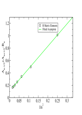
Figure 3: Triangular N2 Matrix elements. The difference $A_{n+1/2}-B_{n}+A_{n+1/2}$ extrapolates to 0.107(1), much lower than $1/z_{t}=0.1726$. The slope with respect to $n^{-2}$ is 3.61(1), much larger than $A/4$. These two observations are consistent with a spectrum edge shift.

We used the transfer matrix method to obtain an exact expansion of the partition function in powers of the activity. We have constructed transfer matrices for strips with width up to $M=26$ (number of symmetry reduced states in the $M=26$ matrix is 730100). We then constructed the exact low-$z$ power series expansion for the density $\rho(z)$, the first 17 coefficients of which are identical with their bulk values (the cluster integrals for the models considered henceforth and the resulting $R$ matrices are given in tables 1, 2). The difference $A_{n-1/2}+A_{n+1/2}-B_{n}$ should converge to $2A-B=z_{t}^{-1}$. In the absence of oscillatory terms, the slope of this difference against $1/n^{2}$ determines the critical exponent by (I). As seen in figure 3 the matrix elements are well fitted, with $2A-B=0.107(1)$ and $2a-b=3.61(1)$, and extrapolation of $A_{n}$ alone gives $A=5.382$. Therefore, in this case analysis of the R matrix shows clearly that $4(2a-b)/A\simeq 2.7>1$ which means that (11) will lead to an imaginary $\sigma^{\prime}$. As discussed above, in such cases the above analysis breaks down as the spectrum edge shifts from $2A\pm B$. Indeed, for this model the critical activity as determined by MC studies, $z_{t}=5.794$ zhang , deviates significantly from $(2A-B)^{-1}=9.35$, clearly demonstrating the spectrum edge shift.

IV.3 Square lattice N4 model

Having tested the limits of the method, we move on to apply it and examine models in which the critical behavior is not known. The N4 model on a square lattice (hard-core exclusion of all neighbors up to the $4^{th}$ order) was first studied using transfer matrix methods orbanphd ; nisbet . Recently, it was revisited, employing MC simulations levin . It is believed to undergo a second order fluid-solid transition of the Ising universality class. The critical chemical potential was found to be $\mu_{c}=4.705$ with a critical density $\rho_{c}=0.110$ levin , where the closest packing density is $\rho_{cp}=0.125$.

Here too, we used the transfer matrix method to obtain an exact expansion of the partition function and expand the density in powers of the activity. We have constructed transfer matrices for strips with width up to $M=37$. Employing translational and inversion symmetries, the number of symmetry reduced states in the $M=37$ matrix is 4137859. Using this matrix, we obtained the first 18 coefficients that are identical with the bulk values. The diagonal matrix elements take the form $B+b/n^{2}+b^{\prime}\cos(qn+\phi)/n$, while the off-diagonal ones exhibit no visible oscillations, and are well fitted by the cubic form $A+a/n^{2}+a^{\prime\prime}/n^{3}$ (see figure 4). Based on the fit parameters, one is able to predict the non-physical singularity location $-z_{0}=-0.0294$, which compares well with the value we obtained from direct ratio analysis of the series $-z_{0}=-0.029374(1)$. The critical exponent at this singularity is calculated by I to be $\sigma=0.1891$, close to the exact universal value $\sigma=1/6$.

Looking at the physical singularity, one observes $2A-B=0.015(5)$, i.e., $\mu_{c}=4.2(4)$, barely consistent with the result of levin . While the accuracy in determining the critical activity is low, the critical density can be determined to much better accuracy $\rho_{c}=0.112(1)$, in good agreement with the MC results. It is remarkable that we are able to determine to such accuracy the critical density at the fluid-solid transition based on the low-density behavior of the fluid alone. The critical exponent may be found by (I) to be $\sigma^{\prime}=0.28(6)$. Thus, based on our analysis of the cluster integrals we can quite safely exclude the possibility of the Ising universality class, where $\sigma^{\prime}=1$. The latter result contradicts the numerical observations of levin . Detailed numerical studies of this model aimed at an accurate calculation of the critical exponents are required to settle this discrepancy.

IV.4 Square lattice N5 model

Finally, we look at the N5 model on a square lattice (hard-core exclusion of all neighbors up to the $5^{th}$ order). This model was also recently studied using MC simulations levin and found to undergo a weak first order transition at $\mu_{c}=5.554$. Again, we calculated 18 cluster coefficients using the transfer matrix method up to $M=37$. In this case, one observes no oscillations, but the $R$ matrix elements exhibit a strong third-order correction term: $A_{n}=A+a/n^{2}+a^{\prime\prime}/n^{3}$ and $B_{n}=B+b/n^{2}+b^{\prime\prime}/n^{3}$ (see figure 5). While the third order term is stronger than the second-order one in the regime studied, our RG analysis allows us to conclude that the $1/n^{3}$ correction does not change the critical exponents and we can use (11). The non-physical exponent $\sigma$ calculated from the above parameters, $\sigma=0.1718$ is in reasonable agreement with the exact universal result $1/6$. Similar calculation for the physical singularity yields $\sigma=0.1621$. The accuracy of the latter result might suffer from the lack of insufficient cluster integrals. However, one can safely say that the diagonal $1/n^{2}$ amplitude $b$ is small, and thus the physical exponent $\sigma^{\prime}$ would not deviate much from $\sigma$, and should satisfy $\sigma^{\prime}\simeq 1/6$. The critical activity $z_{t}=(2A-B)^{-1}$ is estimated to be $z_{t}=166$, but is highly sensitive to small errors in $A$ and $B$ and might be very well equal or higher than the one reported in levin ($z_{c}=258$). If $z_{t}>z_{c}$ then the critical point we found corresponds to the termination of the super-cooled fluid phase. This scenario is discussed in eliasher and was suggested to be related to a glass transition eliasher ; eli .

V Conclusion

The $R$ matrix representation of the Mayer cluster integrals converges very quickly to its asymptotic form. It therefore provides a powerful tool for extrapolating the low-$z$ expansion of the fluid equation of state to cover the full fluid regime. In this work we analyze the analytic properties of this equation of state in the vicinity of the critical points. It is shown that not only the location of the critical points, but also the critical exponents can be determined if one identifies correctly the asymptotic behavior of the $R$ matrix elements. A number of correction forms are analyzed, most of which are shown by RG arguments to be irrelevant for the critical behavior. Thus, we provide an exact formula for the critical exponents, depending on a relatively few parameters characterizing the functional dependence of the matrix elements. Application of this method to a number of lattice-gas models results in partial agreement with recent MC studies. Analysis of the discrepancies through an extensive MC study is left for future work.

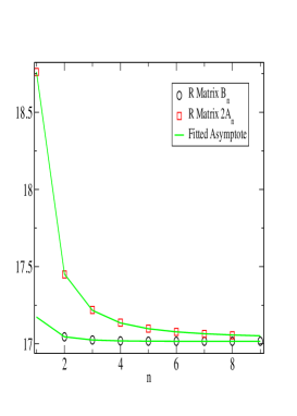
Figure 4: N4 Matrix elements. The diagonal terms are fitted to the functional form (2): $B=17.0121$, $b=0.19$, $b^{\prime}=0.029$, $q=0.295$. The off diagonal term fit well (1) with an added cubic correction $a^{\prime\prime}/n^{3}$: $2A=17.0316$, $2a=1.634$, $2a^{\prime}=0$, $2a^{\prime\prime}=0.0957$.

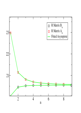
Figure 5: N5 Matrix elements. Diagonal and off-diagonal terms fit well (1) with an added cubic correction $b^{\prime\prime}/n^{3}$ ($a^{\prime\prime}/n^{3}$) : $B=20.547$, $b=-0.0166$, $b^{\prime\prime}=-0.706$. $2A=20.553$, $2a=2.28$, $2a^{\prime\prime}=0.143$.

VI Appendix A: Construction of the $R$-matrix

Here we give an explicit recursive construction of a tridiagonal symmetric $R$ matrix that satisfies (5). First, assign

$$R_{11}=-2b_{2}.$$

Assuming all elements $R_{ij}$ are known for $1\leq i,j\leq m$ (and (5) is satisfied for $n\leq 2m$), we construct $R_{m,m+1}$ and $R_{m+1,m+1}$ as follows:

Define $P$ to be the $m\times m$ leading submatrix of $R$, i.e., the first $m$ rows and first $m$ columns of $R$. The next off-diagonal element is given by

$$R_{m,m+1}^{2}=R_{m+1,m}^{2}=\frac{(2m+1)b_{2m+1}-(P^{2m})_{11}}{(P^{m-1})_{1m}^{2}}.$$

Now define $Q$ to be the $(m+1)\times(m+1)$ leading submatrix of $R$, with zero as its $m+1,m+1$ element. The next diagonal element is then given by

$$R_{m+1,m+1}=\frac{-(2m+2)b_{2m+2}-(Q^{2m+1})_{11}}{(Q^{m})_{1,m+1}^{2}}.$$

It is easy to see by explicit multiplication that the submatrix up to row and column $m$ satisfy (5) up to $n=2m$. Further matrix elements do not affect $(R^{j})_{11}$ for $j\leq n$. Therefore, each additional cluster integral allows for one additional $R$ matrix elements. It should be pointed out that the above process is exponentially sensitive to errors. This means that if one is interested in matrices with $m>5$ or so, the cluster integrals used should be exact or at least known to high accuracy. In addition, the actual construction of $R$ matrices should generally be done using high-accuracy arithmetics to avoid build-up of round-off errors.

VII Appendix B

We first show that

$$\prod\limits_{j=1}^{N}[1+\cos(2^{j-1}q)]^{2}\simeq 4^{-N},\quad\quad(N\to\infty).$$ (21)

Taking the logarithm of the product, one obtains $2\sum\limits_{j=1}^{N}\ln[1+\cos(2^{j-1}q)]$. It is easy to see that for $q/(2\pi)$ irrational, the sequence $2^{j}q(\mod 2\pi)$ is uniformly dense in $(0,2\pi)$. Thus, in the limit $N\to\infty$ the sum may be replaced by an integral

$$2\sum\limits_{j=1}^{N}\ln[1+\cos(2^{j-1}q)]=2N\int\limits_{0}^{2\pi}\ln[1+\cos(x)]dx=-2N\ln(2).$$

Exponentiating the result, one reveals (21).

Secondly, we show that

$$f(q)=1+\sum\limits_{i=1}^{\infty}\prod\limits_{j=1}^{i}[1+\cos(2^{j-1}q)]^{2}=\frac{2}{1-\cos(q)}.$$ (22)

It follows from the definition that $f(q)$ satisfies $f(q)-1=[1+\cos(q)]^{2}f(2q)$. This recursion rule is indeed satisfied by $f(q)=2/[1-\cos(q)]$. All left to be shown is that there is no other (continuous) solution. Assume there exist two different solutions $f_{1}(q)$ and $f_{2}(q)$. Their difference $\delta f(q)=f_{1}(q)-f_{2}(q)$ then satisfies

$$\delta f(q)=[1+\cos(q)]^{2}\delta f(2q)=\delta f(2^{n}q)\prod\limits_{j=1}^{n}[1+\cos(2^{j-1}q)]^{2}$$ (23)

Let $q/(2\pi)$ be irrational. $\delta f$ is continuous, thus for each $\epsilon$ there exists $\delta$ such that $|q_{1}-q|<\delta\to|f(q_{1})-f(q)|<\epsilon$. Again we use the fact that the sequence $2^{j}q(\mod 2\pi)$ is uniformly dense in $(0,2\pi)$ to deduce that there exists also $N$ such that $|2^{N}q(\mod 2\pi)-q|<\delta$ and thus $|\delta f(2^{N}q)-\delta f(q)|<\epsilon$. In fact there are infinitely many such $N$’s, so one may find $N$ as large as required to satisfy the latter inequality, while at the same time satisfying (21). Employing (23) one finds

$$\delta f(q)=\delta f(2^{N}q)\prod\limits_{j=1}^{N}[1+\cos(2^{j-1}q)]^{2}\sim 4^{-N}\delta f(2^{N}q).$$ (24)

That is, $|f(2^{N}q)-f(q)|\simeq(4^{N}-1)|f(q)|>>\epsilon$ in contradiction to the abode, unless $\delta f(q)=0$. Since this is true for all irrational $q/(2\pi)$, the function must vanish identically if continuous. Q.E.D.

References

- (1) L. Onsager, Ann. N.Y. Acad. Sci. 51, 627 (1949).
- (2) R. Zwanzig, J. Chem. Phys. 39, 1714 (1963).
- (3) B.J. Alder and T.E. Wainwright, Phys. Rev. 127, 357 (1962).
- (4) W.W. Wood and J.D. Jacobson, J. Chem. Phys. 27, 1207 (1957).
- (5) B.J. Alder and T.E Wainwright, J. Chem. Phys. 33, 1439 (1960).
- (6) W.G. Hoover and F.H. Ree, J. Chem. Phys. 49, 3609 (1968).
- (7) P.J. Michels and N.J. Trappaniers, Phys. Lett. A 104, 425 (1984).
- (8) D.R. Nelson and B.I. Halperin, Phys. Rev. B 19, 2457 (1979).
- (9) A.P. Young, Phys. Rev. B 19, 1855 (1979).
- (10) J. Groeneveld, Phys. Lett. 3, 50 (1962).
- (11) A. Baram and J.S. Rowlinson, J. Phys. A 23, L399 (1990).
- (12) A. Baram and M.J. Fixman, J. Chem. Phys. 101, 3172 (1994).
- (13) A. Baram and J.S. Rowlinson, Mol. Phys. 74, 707 (1991).
- (14) E. Eisenberg and A. Baram, Phys. Rev. E 73, 025104(R) (2006).
- (15) A. Baram and M. Luban, Phys. Rev. A 36, 760 (1987).
- (16) S.N. Lai and M.E. Fisher, J. Chem. Phys. 103, 8144 (1995).
- (17) Y. Park and M.E. Fisher, Phys. Rev. E 60, 6323 (1999).
- (18) E. Eisenberg and A. Baram, PNAS 104, 5755 (2007).
- (19) R.J. Baxter, J. Phys. A: Math. Gen. 13, L61 (1980).
- (20) H.C.M. Fernandes, J.J. Arenzon and Y. Levin, J. Chem. Phys. 126, 114508 (2007).
- (21) T.M. Dunster, SIAM J. Math. Anal. 21, 995-1018 (1990).
- (22) A.J. Guttmann, Phase Transition and Critical Phenomena, vol. 13, ed. C. Domb and J. Lebowitz (New York: Academic)
- (23) G.S. Joyce, Phil. Trans. Royal Soc. London A 325, 643-702 (1988).
- (24) The exact 1100 cluster integrals , and the first 550 matrix elements are available on-line at http://star.tau.ac.il/eli/Rmat .
- (25) J. Orban and A. Bellemans, J. Chem. Phys. 49, 363 (1968).
- (26) L.K. Runnels, J.R. Craig, and H.R. Stereiffer, J. Chem. Phys. 54, 2004 (1971).
- (27) R.M. Nisbet and I.E. Farquhar, Physica (Amsterdam) 76, 283 (1974).
- (28) N.C. Bartelt and T.L. Einstein, Phys. Rev. B 30, 5339 (1984).
- (29) W. Zhang and Y. Deng, Phys Rev E 78, 031103 (2008).
- (30) J. Orban, Ph.D. thesis, Universite Libre de Bruxelles (1969).
- (31) E. Eisenberg and A. Baram, Europhys. Lett. 71, 900 (2005)