On the role of the curvature drift instability in the dynamics of electrons in active galactic nuclei

Abstract

We study the influence of the centrifugally driven curvature drift instability (CDI) on the dynamics of relativistic electrons in the magnetospheres of active galactic nuclei (AGN). We generalize our previous work by considering relativistic particles with different initial phases. Considering the Euler, continuity, and induction equations, by taking into account the resonant conditions, we derive the growth rate of the CDI. We show that due to the centrifugal effects, the rotational energy is efficiently pumped directly into the drift modes, that leads to the generation of a toroidal component of the magnetic field. As a result, the magnetic field lines transform into such a configuration when particles do not experience any forces and since the instability is centrifugally driven, at this stage the CDI is suspended.

PACS numbers: 95.30.Qd; 98.62.Js; 94.20.wc

1 Introduction

Usually in AGN magnetospheres the magnetic field varies in the following interval $10^{2}-10^{4}$G depending on the distance from the black hole event horizon. Therefore, magnetic field is very strong and leads to the frozen-in condition of plasmas. This means that plasma particles are forced to follow magnetic field lines. On the other hand, AGN magnetospheres are characterized by rotational motion and hence, it is clear that one has to study how the plasma goes through the light cylinder surface (LCS) (a hypothetical zone where the linear velocity of rigid rotation exactly equals the speed of light). It is evident that if the rigid rotation is preserved, sooner or later the physical system will encounter violation of the causality principle. Therefore, in the mentioned zone, a certain twisting process of magnetic field lines must exist, by means of which, the particles will lag behind the rotation avoiding the aforementioned problem. In Ref. r03 authors considered curved trajectories and generalized a work developed by Machabeli & Rogava (see Ref. mr). The authors examined a single particle, sliding along a corotating, curved channel. In this simple mechanical model the channel plays a role of magnetic field lines. It was shown that dynamics of particles asymptotically becomes force-free if a shape of the channel is given by the Archimedes’ spiral and the particles cross the LCS without violating the causality principle.

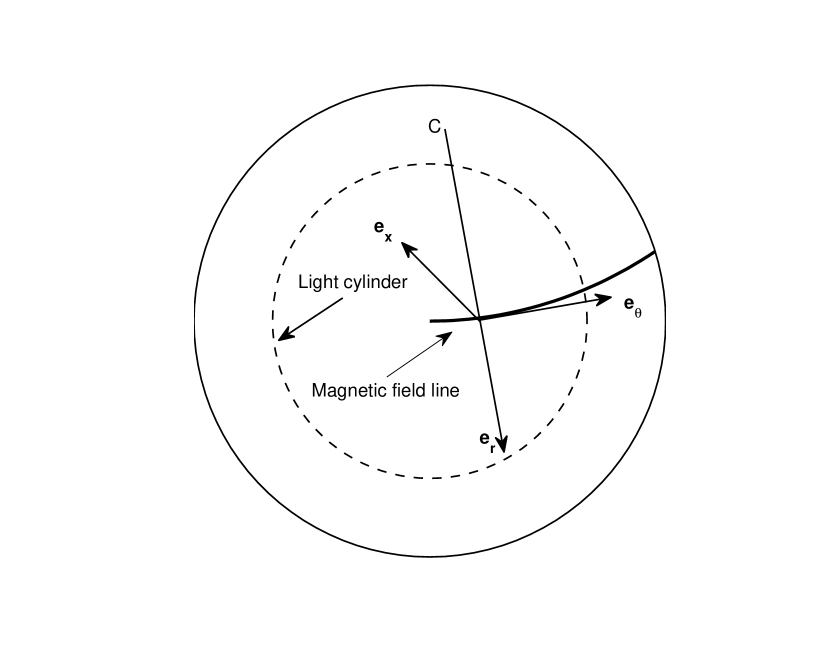
Figure 1: The geometry in which the set of main Eqs. (2-4) is considered; (${\bf e}_{\theta},{\bf e}_{r},{\bf e}_{x}$) denotes orthonormal basis of unit vectors; ${\bf e}_{x}$ is directed perpendicularly to the plane of the figure (equatorial plane); $C$ is the center of the curvature; and ${\bf e}_{\theta}$ and ${\bf e}_{r}$ are the tangential and perpendicular (with respect to the field line) unit vectors respectively.

Generally speaking, if the magnetic field is still robust, one has to twist the field lines in an appropriate way. Therefore, it is necessary to generate the toroidal component of the magnetic field provided by certain current. It is well known that particles moving along curved field lines, also drift perpendicularly to the curvature plane even if the curvature is very small. Such a drift motion creates curvature current, which leads to the development of the CDI (see e.g., Ref. shmmkh03).

As we have already mentioned, the innermost region of AGN magnetospheres is supposed to be rotating, therefore, the centrifugal force (CF) must be essential for studying the magnetospheric plasma motion. Magneto-centrifugal effects have been studied in a series of papers. Blandford and Payne considered the angular momentum and energy pumping process from accretion disks (Ref. bp82). The authors emphasized a special role of CF in dynamical processes governing the acceleration of plasmas. The role of the centrifugal acceleration in producing the non-thermal radiation from rotating AGN winds has been studied in Ref. gl97. This work has been generalized in Ref. osm7 and it has been shown that under certain conditions electrons might reach very high Lorentz factors $10^{5-8}$. The similar investigation performed for non-blazar objects was developed in Ref. ra8 and the high efficiency of centrifugal acceleration was emphasized.

Generally speaking, the centrifugal acceleration may induce plasma instabilities. When the CF acts on a particle and changes in time, it plays a role of a parameter, and drives the so-called parametric instability. Centrifugally excited unstable plasma waves deserve a special interest in different astrophysical scenarios. In Ref. incr1 the authors considered the corotating Crab magnetsphere arguing that the centrifugal force inevitably causes the separation of charges, that in turn leads to the creation of the Langmuir waves. We have shown that due to the centrifugal effects the instability is very efficient. This method was applied to AGN jets in Ref. incr3 and the stability problem of the rotation-induced electrostatic waves has been studied. The CF is significant also for inducing the CDI. Even if the field lines have a very small curvature, it might cause a drifting process of plasma, creating current, which will inevitably produce the toroidal component of the magnetic field. However, a value of the mentioned component is not strong enough to change a field line’s configuration significantly. In this context corotation plays an important role. In particular, as is shown in our model by means of the centrifugal acceleration, the rotational energy can be pumped directly into the toroidal component, amplifying it efficiently. This is the meaning of the curvature drift instability. For examining the role of the corotation in the curvature drift instability for pulsar magnetospheres, in Ref. mnras we studied the two-component relativistic plasma, estimating the increment of the instability. We have found that the growth rate was bigger than pulsar’s spin-down rate by many orders of magnitude, indicating high efficiency of the CDI. This instability is very important since, due to the mentioned drift, current is produced, which, via the parametric mechanism leads to the creation of the amplifying toroidal magnetic field, reconstructing the magnetosphere. By the influence of the toroidal magnetic field, the initial field lines are twisting until they transform into the shape of the Archimedes spiral, when the motion of the particles is described by the so-called force-free regime (see Ref. ff). The similar problem, thus excitation of the CDI in AGN magnetospheres was studied in Ref. agnff and it has been shown that the instability is very efficient and might strongly influence processes in AGN plasmas. The major restriction of this work was that we have studied particles with exactly equal initial phases, and it is clear that most of the electrons have different values of phases. In the present paper is we address two goals: (a) we examine the contribution of electrons with different phases in generation of toroidal magnetic field and (b) study the influence of the induced magnetic field on dynamics of particles.

The paper is arranged as follows. In Sect. 2, we introduce the curvature drift waves and derive the dispersion relation and a corresponding expression of the transition timescale. In Sect. 3, the results for typical parameters of AGN are presented and, in Sect. 4, we summarize our results.

2 Excitation of curvature drift waves

In AGN magnetospheres the relativistic electrons have energies in a broad interval. We consider plasma that consists of relativistic electrons with the following Lorentz factors $\gamma\sim 10^{5-8}$ Ref. osm7,ra8. It is assumed that the field lines initially are almost rectilinear and corotate. As we have already mentioned in the introduction, current providing the twisting of field lines is created due to the curvature drift, characterized by the following (curvature drift) velocity

$$u=\frac{\gamma_{0}v_{{}_{\parallel}}^{2}}{\omega_{B}R_{B}},$$ (1)

where $\omega_{B}=eB_{0}/mc$, $e$ and $m$ are particle’s charge and the rest mass respectively, $B_{0}$ is the unperturbed magnetic induction, $c$ is the speed of light, $R_{B}$ is the curvature radius of magnetic field lines, $\gamma_{0}$ is the initial Lorentz factor of particles and $v_{{}_{\parallel}}$ is the longitudinal velocity. As it is clear from Eq. (1), the drift velocity is proportional to $\gamma_{0}m$, therefore, the corresponding value of the bulk flow (protons) (having the Lorentz factor of the order of $10$), will be by many orders of magnitude less than that of the relativistic electrons (with $\gamma_{0}\sim 10^{5-8}$). This in turn means that the contribution of protons is negligible and we consider one-component plasma composed of relativistic electrons.

In the zeroth approximation, particles move along the magnetic field lines and our aim is to consider the twisting process of these field lines and study a subsequent saturation mechanism.

The CDI is centrifugally driven and therefore, for studying the development of the twisting process of magnetic field lines we consider the Euler equation, which governs the dynamics of corotating plasma particles (see Ref. incr1)

$$\frac{\partial{\bf p}}{\partial t}+({\bf v\cdot\nabla)p}=-c^{2}\gamma\xi{\bf\nabla}\xi+\frac{e}{m}\left({\bf E}+\frac{1}{c}\bf v\times\bf B\right),$$ (2)

where

$$\xi\equiv\sqrt{1-\Omega^{2}R^{2}/c^{2}},$$

and ${\bf p}$ is the momentum, ${\bf v}$ is the velocity, ${\gamma}$ is the Lorentz factor of the relativistic particles, and ${\bf E}$ and ${\bf B}$ are the electric field and the magnetic induction, respectively. $\Omega$ is the angular velocity of rotation and $R$ is the coordinate along the magnetic field lines. We express the equation of motion in the cylindrical coordinates (see Fig. 1). The first term on the right-hand side of the Euler equation $-c^{2}\gamma\xi{\bf\nabla}\xi$ represents the centrifugal force per unit mass. As we see, this force becomes asymptotically infinity on the LCS, therefore, its overall effect is significant in the mentioned zone. For closing the system, we add to Eq. (2) the continuity equation:

$$\frac{\partial\rho}{\partial t}+{\bf\nabla}\cdot{\bf J}=0,$$ (3)

and the induction equation:

$${\bf\nabla\times B}=\frac{1}{c}\frac{\partial{\bf E}}{\partial t}+\frac{4\pi}{c}{\bf J},$$ (4)

respectively. By $\rho\equiv en$ and ${\bf J}\equiv en{\bf v}$ we denote the charge density and the current density, respectively and $n$ represents the electron number density.

If we take into account the frozen-in condition, $\bf E_{0}+\bf v_{0}\times\bf B_{0}/c=0$, describing the leading state of the system, then one can show that Eq. (2) reduces to [2]:

$$\frac{dv}{dt}=\frac{\Omega^{2}R}{1-\frac{\Omega^{2}R^{2}}{c^{2}}}\left[1-\frac{\Omega^{2}R^{2}}{c^{2}}-\frac{2v^{2}}{c^{2}}\right].$$ (5)

Machabeli & Rogava have shown that for the ultra relativistic case ($\gamma>>1$) the radial velocity, $v\equiv dR/dt)$ behaves as follows (see Ref. mr)

$$v(t)\equiv v_{{}_{\parallel}}\approx c\cos(\Omega t+\varphi),$$ (6)

where $\varphi$ denotes the initial phase of a particle. As we have already mentioned in the introduction, one of the goals of the present work is to take into account relativistic electrons with different values of $\varphi$ and see the corresponding net effect.

We assume that the magnetic field lines initially have a small curvature, that drives the particles along the $x$ axis (see Fig. 1). The drift causes current, which in turn creates the toroidal component of the magnetic field.

For studying the development of the CDI following the method described in Reef. mnras,ff,agnff we linearize the system of equations in Eqs. (2-4), by expanding all physical quantities around the leading state

$$\Psi\approx\Psi^{0}+\Psi^{1},$$ (7)

$$\Psi=\{n,{\bf v},{\bf p},{\bf E},{\bf B}\},$$ (8)

where $\Psi^{0}$ and $\Psi^{1}$ denote the zeroth order and the first order quantities respectively. We assume that $n_{0}=const$, $v_{0x}=u$, $v_{0\theta}=v_{{}_{\parallel}}$, ${\bf p_{0}}={\bf v_{0}}/\gamma_{0}$, $B_{0\theta}=B_{0}$, $B_{0r}=B_{0x}=0$, $\bf E_{0}=-\bf v_{0}\times\bf B_{0}/c$. $B_{0}\equiv\sqrt{2L/(R_{c}^{2}c)}$ is the equipartition magnetic field, $L$ is the luminosity of AGN and $R_{c}=c/\Omega$ is the light cylinder radius.

By expressing the perturbed quantities as

$$\Psi^{1}(t,{\bf r})\propto\Psi^{1}(t)\exp\left[i\left({\bf kr}\right)\right]\,,$$ (9)

and taking into account $v^{1}_{r}\approx cE^{1}_{x}/B_{0}$, Eqs. (2-4) reduce to

$$\frac{\partial p^{1}_{x}}{\partial t}-i(k_{x}u+k_{\theta}v_{{}_{\parallel}})p^{1}_{x}=\frac{e}{mc}v_{{}_{\parallel}}B^{1}_{r},$$ (10)

$$\frac{\partial n^{1}}{\partial t}-i(k_{x}u+k_{\theta}v_{{}_{\parallel}})n^{1}=ik_{x}n^{0}v^{1}_{x},$$ (11)

$$-ik_{\theta}cB^{1}_{r}=4\pi e(n^{0}v^{1}_{x}+n^{1}u),$$ (12)

where $k_{x}$ and $k_{\theta}$ are the wave vector components. All vectors are given in terms of the coordinates of the field line (see Fig. 1).

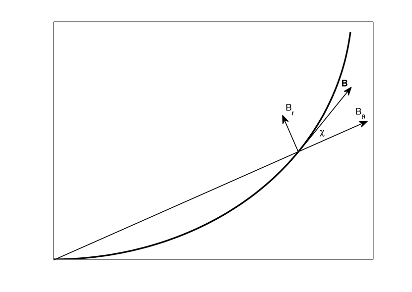
Figure 2: The geometry for deriving Eq. (25): the curved line denotes the twisted magnetic field, ${\bf B}$, generated due to the raising of magnetic perturbation, ${\bf B}_{r}$. Note, that ${\bf B}_{r}$ and ${\bf B}_{\theta}$ are oriented with respect to the initial ‘quasi straight’ magnetic field line.

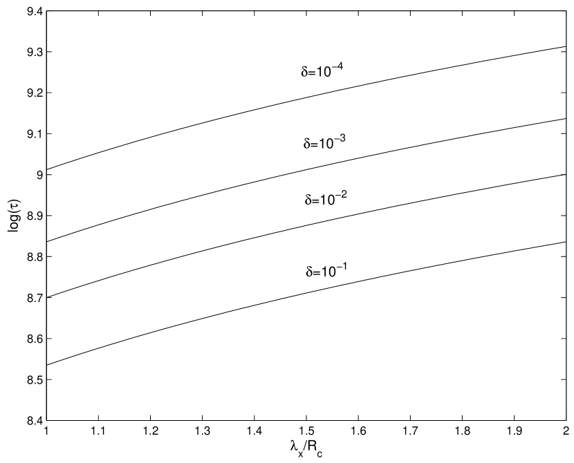
Figure 3: The dependence of logarithm of the transition timescale on the normalized wavelength. The set of parameters is $\Omega=3\times 10^{-5}s^{-1}$, $L/L_{E}=0.01$, $\delta\in\{10^{-1};10^{-2};10^{-3};10^{-4}\}$, $\gamma_{e0}=10^{8}$, $R_{B}\approx R_{c}$, $n_{e0}=0.001cm^{-3}$ and $\lambda_{\theta}\equiv 2\pi/k_{\theta}=100R_{c}$.

Instead of an ansatz used in Ref. agnff, we apply

$$v^{1}_{x}\equiv V_{x}e^{i{\bf kA(t)}},$$ (13)

$$n^{1}\equiv ne^{i{\bf kA}(t)},$$ (14)

$$A_{x}(t)=\frac{ut}{2}+\frac{u}{4\Omega}\sin[2(\Omega t+\varphi)],$$ (15)

$$A_{\phi}(t)=\frac{c}{\Omega}\sin(\Omega t+\varphi),$$ (16)

which differs from that of [12] by considering the nonzero initial phases. By combining Eqs. (13-16) with Eqs. (10-12) one gets an expression describing the development of the toroidal component of the magnetic field

$$-ik_{\phi}cB^{1}_{r}(t)=\frac{\omega^{2}_{e}}{\gamma_{e0}}{\rm e}^{i{\bf kA}(t)}\int^{t}{\rm e}^{-i{\bf kA}(t^{\prime})}v_{{}_{\parallel}}(t^{\prime})B_{r}(t^{\prime})dt^{\prime}+$$

$$i\frac{\omega^{2}_{e}}{\gamma_{e0}}k_{x}u{\rm e}^{i{\bf kA}(t)}\int^{t}dt^{\prime}\int^{t^{\prime\prime}}{\rm e}^{-i{\bf kA}(t^{\prime\prime})}v_{{}_{\parallel}}(t^{\prime\prime})B_{r}(t^{\prime\prime})dt^{\prime\prime}$$

(17)

where $\omega_{e}=e\sqrt{4\pi n_{e0}/m}$ and $n_{e0}$ are the plasma frequency and initial electron number density respectively. The following identity

$${\rm e}^{\pm ix\sin y}=\sum_{s}J_{s}(x){\rm e}^{\pm isy},$$ (18)

where $J_{s}(x)$ ($s=0;\pm 1;\pm 2\ldots$) is the Bessel function of integer order (see Ref. abrsteg) reduces Eq. (17) to

$$B_{r}(\omega,\varphi)=-\frac{\omega_{e}^{2}}{2\gamma_{e0}k_{\theta}c}\sum_{\sigma=\pm 1}\sum_{s,q,l,p}\frac{J_{s}(g)J_{q}(h)J_{l}(g)J_{p}(h)}{\omega+\frac{k_{x}u}{2}+\Omega(2s+q)}\times$$

$$\times B_{r}\left(\omega+\Omega\left(2[s-l]+q-p+\sigma\right)\right)\times$$

$$\times\left[1-\frac{k_{x}u}{\omega+\frac{k_{x}u}{2}+\Omega(2s+q)}\right]\times{\rm e}^{i\varphi\left(2[s-l]+q-p+\sigma\right)}+$$

$$+\frac{\omega_{e}^{2}k_{x}u}{4\gamma_{e0}k_{\theta}c}\sum_{\sigma,\mu=\pm 1}\sum_{s,q,l,p}\frac{J_{s}(g)J_{q}(h)J_{l}(g)J_{p}(h)}{\left(\omega+\frac{k_{x}u}{2}+\Omega(2[s+\mu]+q)\right)^{2}}\times$$

$$\times B_{r}\left(\omega+\Omega\left(2[s-l+\mu]+q-p+\sigma\right)\right)$$

$$\;\;\;\;\;\;\;\;\;\;\;\;\;\;\;\;\;\;\;\;\;\;\;\;\;\;\;\;\times{\rm e}^{i\varphi\left(2[s-l+\mu]+q-p+\sigma\right)},$$ (19)

where

$$g=\frac{k_{x}u}{4\Omega},\;\;\;\;\;\;\;\;\;\;\;\;h=\frac{k_{\theta}c}{\Omega}.$$

For solving Eq. (19) we must examine similar expressions, by rewriting Eq. (19) for the infinite number of components $B_{r}(\omega\pm\Omega,\varphi)$, $B_{r}(\omega\pm 2\Omega,\varphi)$,… etc. Therefore, the system becomes composed of the infinite number of equations, that makes the task unsolvable. On the other hand, by applying physically reasonable cutoff on the-right hand side of the equation, the aforementioned problem disappears. In particular, as we see from the expression the physical system is characterized by the resonance proper frequency

$$\;\;\;\;\;\;\;\;\;\;\;\;\;\;\;\;\;\;\;\;\;\;\;\;\;\;\;\;\;\;\;\;\;\;\;\omega_{0}\approx-\frac{k_{x}u}{2},$$ (20)

$$\frac{k_{x}u}{2}<0,\;2s+q=0,\;2[s+\mu]+q=0.$$

On the other hand, in Ref. agnff it has been shown that AGN magnetospheric parameters satisfy the condition $\omega_{0}/\Omega\ll 1$. This in turn means that all terms with $\Omega(2s+q)$ and $\Omega(2[s+\mu]+q)$ ($2s+q\neq 0$, $2[s+\mu]+q\neq 0$) are rapidly oscillating and do not influence the final result. Therefore, the only contribution comes from $2s+q=0$, $2[s+\mu]+q=0$, which significantly simplifies Eq. (19)

Let us examine an average value of $B_{r}(\omega,\varphi)$ with respect to $\varphi$, which by taking into account

$$\frac{1}{2\pi}\int{\rm e}^{iN\varphi}d\varphi=\delta_{N,0},$$

leads to

$$\left(\omega+\frac{k_{x}u}{2}\right)^{2}\approx$$

$$\approx\sum_{\sigma,\mu=\pm 1}\sum_{s,l}\Xi_{\mu}J_{s}(g)J_{q^{\prime}(s,\mu)}(h)J_{l}(g)J_{p^{\prime}(l,\sigma)}(h),$$ (21)

where

$$\Xi_{0}=2\Xi_{\pm 1}=\frac{\omega^{2}_{e}k_{x}u}{2\gamma_{e0}k_{\theta}c},$$ (22)

$$q^{\prime}=-2(s+\mu),\;\;\;\;\;\;\;p^{\prime}=-2l+\sigma.$$

Expressing $\omega\equiv\omega_{0}+i\Gamma$, one can straightforwardly derive the increment of the CDI

$$\Gamma\approx$$

$$\approx\left[\sum_{\sigma,\mu=\pm 1}\sum_{s,l}\Xi_{\mu}J_{s}(g)J_{-2(s+\mu)}(h)J_{l}(g)J_{-2l+\sigma}(h)\right]^{\frac{1}{2}}.$$ (23)

It is worth noting that this instability is unavoidable for plasma magnetospheric flows, because for the developing of the CDI a) the initial curvature should be nonzero and b) the magnetic field must be robust enough to provide the frozen-in condition. (a)-is a necessary condition for creating the drift waves and (b)-guarantees the parametric mechanism of rotational energy pumping directly into the drift modes.

3 Discussion

Let us consider the Archimedes’ spiral $\Phi=aR$, where $\Phi$ and $R$ are the polar coordinates and $a={\it const}$. As was shown by [1] if the particle slides along the rotating channel that has the shape of the Archimedes’ spiral then, an observer from the laboratory frame of reference will measure the effective angular velocity $\Omega_{ef}=\Omega+d\Phi/dt=\Omega+av$, where $v$ is the radial component of velocity of a particle. In case the motion is force free, thus the particles do not experience any forces, the trajectory in the laboratory frame of reference will be a straight line, characterized by the vanishing effective angular velocity and the following radial velocity, $v=v_{c}\equiv-\Omega/a$. This is an interesting property of the Archimedes’ spiral: if one launches a particle along such a rotating channel (when $a<-\Omega/v_{c}$), then, if the initial radial velocity exactly equals $v_{c}$, the particle will never experience a reaction force, thus, the dynamics of the particle is always force-free. On the other hand, a natural question arises: what happens if the initial velocity differs from $v_{c}$? As is shown in Ref. r03, the radial velocity asymptotically behaves according to the following expression

$$v_{{}_{R}}(R)\rightarrow-\frac{\Omega}{a}+\frac{E\sqrt{a^{2}c^{2}-\Omega^{2}}}{\Omega ca^{2}}\times\frac{1}{R^{2}},$$ (24)

where $E$ is the initial energy of the particle per unit of mass.

Typical AGN outflows are highly relativistic, therefore, let us consider $v_{c}\approx c$ setting $a=-\Omega/c$. Then, as we see from Eq. (24), independently on initial velocity of the the particle, $v_{{}_{R}}$ asymptotically converges to the characteristic velocity, $c$ ($v_{{}_{R}}\rightarrow c$ when $R\rightarrow\infty$). This implies that dynamics of the particle asymptotically becomes force-free. The negative sign of $a$ means that the twisting and rotation have opposite directions and correspondingly electrons moving along such field lines, will lag behind rotation.

Now we can qualitatively analyze how the configuration of magnetic field lines changes with time. After perturbing the magnetic field in the transverse direction, the toroidal component will amplify by means of the energy pumping directly into the waves, caused by the parametric nature of the instability. As a result the field lines will gradually lag behind the rotation. On the other hand, for the twisted field lines, their dynamical influence on particles will decrease due to the vanishing reaction force. In the parallel regime, the efficiency of the CDI will also decrease and when the field lines get a shape of the Archimedes’ spiral the instability completely vanishes. In particular, for this case $\Omega_{ef}\rightarrow 0$ and as a result centrifugal effects are completely damped, the magnetic field lines are saturated, asymptotically providing a relativistic outflow in the force-free regime.

Let us assume that when the particles’ dynamics becomes force-free, the critical value of the toroidal magnetic field is $B_{r}$, then, referring to Fig. 2, by taking into account the property of the Archimedes’ spiral, $\tan\chi=1$ (see Ref. r03), one can show that $\tan\chi=B_{r}/B_{\theta}$. If we apply the exponential temporal behaviour of the toroidal component, $B_{r}\approx B_{r}^{0}\exp(\Gamma\tau)$, then the corresponding transition timescale gets the form

$$\tau\approx-\frac{1}{\Gamma}\ln\left(\frac{B^{0}_{r}}{B_{\theta}}\right).$$ (25)

Generally speaking, the role of the CDI is twofold. On the one hand it guarantees the required twisting of magnetic field lines, and on the other hand, in terms of its feedback on plasma dynamics it provides necessary conditions for the saturation process.

We consider the behaviour of the transition timescale versus the wavelength of the perturbation and the AGN bolometric luminosity respectively. For this purpose let us examine the following parameters: $M_{BH}=10^{8}\times M_{\odot}$, $\Omega=3\times 10^{-5}s^{-1}$ and $L=10^{44}erg/s$, where $M_{BH}$ and $M_{\odot}$ are the AGN mass and the solar mass respectively and $L$ is the bolometric luminosity.

In Fig. 3 we show the logarithm of the saturation timescale versus the wavelength normalized to the light cylinder radius for different values of the initial perturbation $B^{0}_{r}/B_{\theta}\equiv\delta\in\{10^{-1};10^{-2};10^{-3};10^{-4}\}$. The set of parameters is $\Omega=3\times 10^{-5}s^{-1}$, $L/L_{E}=0.01$, $\gamma_{e0}=10^{8}$, $R_{B}\approx R_{c}$, $n_{e0}=0.001cm^{-3}$ and $\lambda_{\theta}\equiv 2\pi/k_{\theta}=100R_{c}$, where $L_{E}=10^{46}erg/s$ is the Eddington luminosity for AGN with the given mass. By different curves we show different cases of initial perturbation. As it is clear from Fig. 3, the transition timescale varies from $\sim 10^{8}s$ ($\lambda_{x}/R_{c}=1$, $\delta=10^{-1}$) to $\sim 10^{9}s$ ($\lambda_{x}/R_{c}=2$, $\delta=10^{-4}$). As we see from the plots, the timescale is a continuously increasing function of $\lambda_{x}(\equiv 2\pi/k_{x})$, which is natural, because by combining Eq. (22) with Eq. (25) one obtains the following behaviour $\tau\propto\sqrt{\lambda_{x}}$.

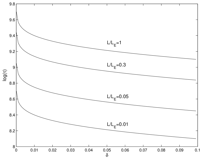
Figure 4: The dependence of logarithm of the transition timescale on the dimensionless perturbation. The set of parameters is $\Omega=3\times 10^{-5}s^{-1}$, $L/L_{E}=\{0.01;0.05;0.3;1\}$, $\gamma_{e0}=10^{8}$, $R_{B}\approx R_{c}$, $n_{e0}=0.001cm^{-3}$, $\lambda_{\theta}\equiv 2\pi/k_{\theta}=100R_{c}$ and $\lambda_{x}=R_{c}$.

In Fig. 4, we display the behaviour of $log(\tau)$ versus the initial perturbation for different values of luminosities. The set of parameters is $\Omega=3\times 10^{-5}s^{-1}$, $L/L_{E}=\{0.01;0.05;0.3;1\}$, $\gamma_{e0}=10^{8}$, $R_{B}\approx R_{c}$, $n_{e0}=0.001cm^{-3}$, $\lambda_{\theta}\equiv 2\pi/k_{\theta}=100R_{c}$ and $\lambda_{x}=R_{c}$. The figure shows the continuously decreasing behaviour of the transition timescale. This is a natural consequence of the fact that for bigger perturbations one needs lower time to reach the critical value $B_{r}$. On the other hand as we see from the plots, the instability is less efficient (bigger timescale) for more luminous AGN. Such a behaviour is clearly seen from an expression of the drift velocity in Eq. (1). In particular, the drift velocity is proportional to the inverse value of the cyclotron frequency, which is bigger for bigger magnetic fields. On the other hand, from an expression of the equipartition magnetic field we have $B_{0}\propto\sqrt{L}$, which means that the curvature drift velocity is proportional to $1/\sqrt{L}$. Since the curvature drift waves are more efficient for bigger curvature drift velocities, by increasing the bolometric luminosity, the increment of the instability will inevitably decrease and the corresponding transition timescale will be larger. For the parameters used for Fig. 4 the transition timescale varies from $\sim 10^{10}s$ ($\delta=10^{-4}$, $L/L_{E}=1$) to $\sim 10^{8}s$ ($\delta=10^{-1}$, $L/L_{E}=0.01$).

Summarizing our results we see that the saturation timescale lies in the range: $\tau\in\{10^{8};10^{10}\}s$. A next step is to specify how efficient is the twisting of field lines. For this purpose it is relevant to examine an accretion process on AGN, estimate the corresponding evolution timescale, and compare it with that of the saturation.

As is shown in Ref. king the accretion timescale is given by

$$t_{evol}=3\times 10^{13}\times\left(\frac{\alpha}{0.3}\right)^{-2/27}\times\left(\frac{\epsilon}{0.1}\right)^{22/27}\times$$

$$\;\;\;\;\;\;\;\;\;\;\times\left(\frac{L}{0.1L_{E}}\right)^{-22/27}\times\left(\frac{M_{BH}}{10^{8}M_{\odot}}\right)^{-4/27}s,$$ (26)

where $\alpha$ is the Shakura-Sunyaev viscosity parameter (see Ref. sak), $\epsilon\equiv L/\dot{M}c^{2}$ is the accretion parameter and $\dot{M}$ denotes the accretion mass rate.

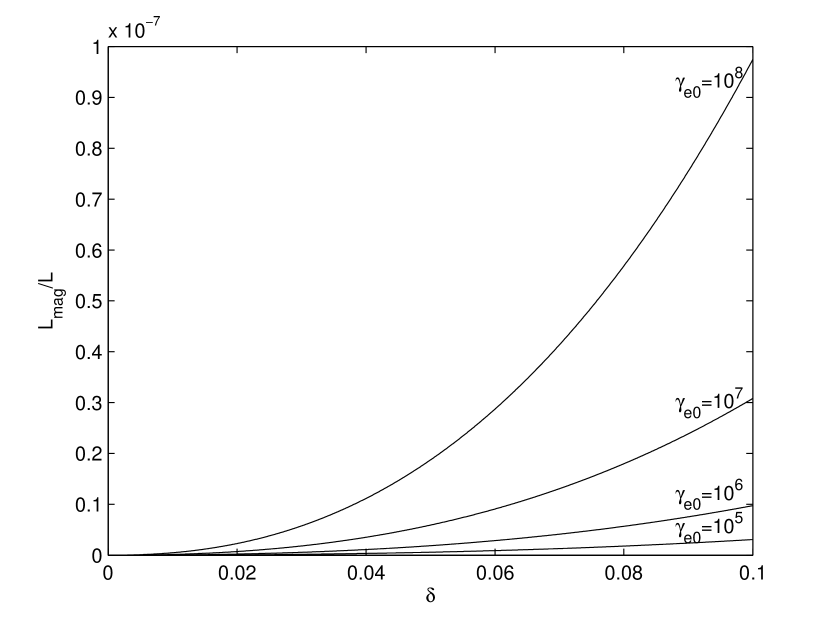
Figure 5: The dependence of $L_{m}/L_{max}$ versus $\delta$. The set of parameters is $\Omega=3\times 10^{-5}s^{-1}$, $L=10^{45}erg/s$, $\gamma_{e0}=\{10^{5};10^{6};10^{7};10^{8}\}$, $R_{B}\approx R_{c}$, $n_{e0}=0.001cm^{-3}$, $\lambda_{\theta}=100R_{c}$ and $\lambda_{x}=R_{c}$.

For typical values, $\alpha=0.3$, $\epsilon=0.1$, one can see that the evolution timescale varies from $\sim 10^{12}s$, ($M_{9}=1$ and $L/L_{E}=1$), to $\sim 10^{14}s$ ($M_{9}=0.001$ and $L/L_{E}=0.01$), where $M_{9}\equiv M_{BH}/(10^{9}\times M_{\odot})$. If one compares these timescales with that of the transition, one finds that $t_{evol}$ exceeds $\tau$ by many orders of magnitude, illustrating the high efficiency of the curvature drift instability.

We have shown that the saturation of the CDI is extremely efficient, however, it is worth noting that the twisting process of magnetic field lines requires a certain amount of energy and a natural question arises: is the energy budget enough to provide the aforementioned process?.

The maximum value of the energy budget per unit of time, being the bolometric luminosity itself, $L_{max}=L$ has to be compared with the ”luminosity” corresponding to the twisting of the magnetic field lines $L_{m}\equiv\Delta E_{m}/\Delta t\approx\Delta E_{m}/\tau$. $\Delta E_{m}$ is the variation in the magnetic energy due to the curvature drift instability.

We consider AGN with $L=10^{45}erg/s$, then, for the reconstruction of the magnetosphere one has to satisfy the condition $L_{m}<L_{max}$. The magnetic ”luminosity” can be estimated straightforwardly

$$L_{m}=\frac{B_{r}^{2}}{4\pi\tau}R_{c}^{3}\kappa,$$ (27)

where $B_{r}$ behaves as

$$B_{r}=B_{r}^{0}e^{t/\tau},$$ (28)

$B_{r}^{0}$ is the initial perturbation of the toroidal component and $\Delta V\approx R_{c}^{2}\Delta R=R_{c}^{3}\kappa$ ($\kappa\equiv\Delta R/R_{c}<<1$) is the volume, where the twisting process takes place.

Let us consider the following set of parameters $\gamma_{e0}=\{10^{5};10^{6};10^{7};10^{8}\}$, $R_{B}\approx R_{c}$, $n_{e0}=0.001cm^{-3}$, $\lambda_{\phi}=100R_{c}$, $\lambda_{x}=R_{c}$ and $L=10^{45}erg/s$. In Fig. 5 we show the dependence $L_{m}/L_{max}$ as a function of the initial perturbation for the moment of the transition ($t\approx\tau$). Different curves correspond to different Lorentz factors. As it is clear from Fig. 5, the total luminosity budget, exceeds, by many orders of magnitude, the magnetic luminosity, indicating that this process is feasible.

4 Summary

We summarize the principal steps and conclusions of our study to be:

1. We have studied the curvature drift instability and its influence on the dynamics of relativistic electrons in AGN magnetospheres.

2. By linearizing the Euler, continuity and induction equations we have derived the dispersion relation of the parametrically excited curvature drift instability and obtained an expression of the growth rate for the light cylinder area. The study was performed by generalizing the previous work and taking into account different initial phases of relativistic particles.

3. As a next step we have estimated the transition timescale of quasi-linear configuration of magnetic field lines into the Archimedes spiral. Such a shape of field lines guarantees the force-free dynamics of particles and necessarily provides the saturation of the instability.

4. We have shown that the transition timescale was lower by many orders of magnitude than the accretion evolution timescale, illustrating extremely high efficiency of the CDI.

5. Analyzing the energy budget, it has been shown that the reconstruction of the magnetic field lines (which in turn provides the force-free regime of electrons) requires only a tiny fraction of the total energy budget, indicating that the CDI is a working process and the corresponding transition to force-free dynamics is the realistic process.

In the framework of the present paper two major restrictions have been considered: (a) a single particle approach and (b) magnetic field lines located in the equatorial plane. Therefore, it is clear that a corresponding generalization of the work is needed and we will investigate it in future studies.

References

- [1] A. D., Rogava, G. Dalakishvili & Z. Osmanov, Gen. Rel. and Grav. 35 (2003) 1133
- [2] G. Machabeli & A. D. Rogava, Phys.Rev. A 50 (1994) 98
- [3] D. Shapakidze, G. Machabeli, G. Melikidze & D. Khechinashvili, Phys.Rev. E 67 (2003) 026407
- [4] R. D. Blandford & D. G. Payne, Mon. Not. R. Astron. Soc. 199 (1982) 883
- [5] R. T. Gangadhara & H. Lesch, Astron. Astrophys. 323 (1997) L45
- [6] Z. Osmanov, A. D. Rogava & G. Bodo, Astro. Astrophys. 470 (2007) 395
- [7] F. M. Rieger & F. A. Aharonian, Astron. Astrophys. 479 (2008) 5
- [8] G. Machabeli, Z. Osmanov & S. Mahajan, Phys. Plasmas 12 (2005) 062901
- [9] Z. Osmanov, Phys. Plasmas 15 (2008) 032901
- [10] Z. Osmanov, G. Dalakishvili & G. Machabeli, Mon. Not. R. Astron. Soc. 383 (2008) 1007
- [11] Z. Osmanov, D. Shapakdze & G. Machabeli, Astron. Astrophys. 503 (2008) 19
- [12] Z. Osmanov, Astron. Astrophys. 490 (2008) 487
- [13] M. Abramovitz & I. Stegan, Handbook of Mathematical Functions, (eds.: Dover Publications Inc.: New York) (1965) 320
- [14] N. I. Shakura & R. A. Sunyaev, Astron. Astrophys. 24 (1973) 337
- [15] A. R. King & J. E. Pringle, Mon. Not. R. Astron. Soc. 377 (2007) 25