Parametric Packing of Selfish Items and the Subset Sum Algorithm

Abstract

The subset sum algorithm is a natural heuristic for the classical Bin Packing problem: In each iteration, the algorithm finds among the unpacked items, a maximum size set of items that fits into a new bin. More than 35 years after its first mention in the literature, establishing the worst-case performance of this heuristic remains, surprisingly, an open problem.

Due to their simplicity and intuitive appeal, greedy algorithms are the heuristics of choice of many practitioners. Therefore, better understanding simple greedy heuristics is, in general, an interesting topic in its own right. Very recently, Epstein and Kleiman (Proc. ESA 2008, pages 368-380) provided another incentive to study the subset sum algorithm by showing that the Strong Price of Anarchy of the game theoretic version of the bin-packing problem is precisely the approximation ratio of this heuristic.

In this paper we establish the exact approximation ratio of the subset sum algorithm, thus settling a long standing open problem. We generalize this result to the parametric variant of the bin packing problem where item sizes lie on the interval $(0,\alpha]$ for some $\alpha\leq 1$, yielding tight bounds for the Strong Price of Anarchy for all $\alpha\leq 1$. Finally, we study the pure Price of Anarchy of the parametric Bin Packing game for which we show nearly tight upper and lower bounds for all $\alpha\leq 1$.

1 Introduction

Motivation and framework. The emergence of the Internet and its rapidly gained status as the predominant communication platform has brought up to the surface new algorithmic challenges that arise from the interaction of the multiple self-interested entities that manage and use the network. Due to the nature of the Internet, these interactions are characterized by the (sometimes complete) lack of coordination between those entities. Algorithm and network designers are interested in analyzing the outcomes of these interactions. An interesting and topical question is how much performance is lost due to the selfishness and unwillingness of network participants to cooperate. A formal framework for studying interactions between multiple rational participants is provided by the discipline of Game Theory. This is achieved by modeling the network problems as strategic games, and considering the quality of the Nash equilibria of these games. In this paper we consider pure Nash equilibria and strong equilibria. These equilibria are the result of the pure strategies of the participants of the game, where they choose to play an action in a deterministic, non-aleatory manner.

The algorithmic problems that are usually studied from a game theoretic point of view are abstractions of real world problems, typically dealing with basic issues in networks. In this paper, we consider game theoretic variants of the well-known Bin Packing problem and its parametric version; see [5, 4, 6] for surveys on these problems.

In the classic Bin Packing problem, we are given a set of items $I=\{1,2,\ldots,n\}$. The $i$th item in $I$ has size $s_{i}\in(0,1]$. The objective is to pack the items into unit capacity bins so as to minimize the number of bins used. In the parametric case, the sizes of items are bounded from above by a given value. More precisely, given a parameter $\alpha\leq 1$ we consider inputs in which the item sizes are taken from the interval $(0,\alpha]$. Setting $\alpha$ to 1 gives us the standard Bin Packing problem.

As discussed in [8], bin packing is met in a great variety of networking problems, such as the problem of packing a given set of packets into a minimum number of time slots for fairness provisioning and the problem of packing data for Internet phone calls into ATM packets, filling fixed-size frames to maximize the amount of data that they carry. This fact motivates the study of Bin Packing from a game theoretic perspective. The Parametric Bin Packing problem also models the problem of efficient routing in networks that consist of parallel links of same bounded bandwidth between two terminal nodes—similar to the ones considered in [14, 2, 8]. As Internet Service Providers often impose a policy which restricts the amount of data that can be downloaded/uploaded by each user, placing a restriction on the size of the items allowed to transfer makes the model more realistic.

The model. In this paper we study the Parametric Bin Packing problem both in cooperative and non-cooperative versions. In each case the problem is specified by a given parameter $\alpha$. The Parametric Bin Packing game is defined by a tuple $BP(\alpha)=\langle N,(B_{i})_{i\in N},(c_{i})_{i\in N}\rangle$. Where $N$ is the set of the items, whose size is at most $\alpha$. Each item is associated with a selfish player—we sometimes consider the items themselves to be the players. The set of strategies $B_{i}$ for each player $i\in N$ is the set of all bins. Each item can be assigned to one bin only. The outcome of the game is a particular assignment $b=(b_{j})_{j\in N}\in\times_{j\in N}B_{j}$ of items to bins. All the bins have unit cost. The cost function $c_{i}$ of player $i\in N$ is defined as follows. A player pays $\infty$ if it requests to be packed in an invalid way, that is, a bin which is occupied by a total size of items which exceeds 1. Otherwise, the set of players whose items are packed into a common bin share its unit cost proportionally to their sizes. That is, if an item $i$ of size $s_{i}$ is packed into a bin which contains the set of items $B$ then $i$’s payment is $c_{i}=s_{i}/\sum_{k\in B}s_{k}$. Notice that since $\sum_{k\in B}s_{k}\leq 1$ the cost $c_{i}$ is always greater or equal than $s_{i}$. The social cost function that we want to minimize is the number of used bins.

Clearly, a selfish item prefers to be packed into a bin which is as full as possible. In the non-cooperative version, an item will perform an improving step if there is a strictly more loaded bin in which it fits. At a Nash equilibrium, no item can unilaterally reduce its cost by moving to a different bin. We call a packing that admits the Nash conditions $NE$ packing. We denote the set of the Nash equilibria of an instance of the Parametric Bin Packing game $G\in BP(\alpha)$ by $NE(G)$.

In the cooperative version of the Parametric Bin Packing game, we consider all (non-empty) subgroups of items from $N$. The cost functions of the players are defined the same as in the non-cooperative case. Each group of items is interested to be packed in a way so as to minimize the costs for all group members. Thus, given a particular assignment, all members of a group will perform a joint improving step (not necessarily into a same bin) if there is an assignment in which, for each member, the new bin will admit a strictly greater load than the bin of origin. The costs of the non-members may be enlarged as a result of this improving step. At a strong Nash equilibrium, no group of items can reduce the costs of all its members by moving to different bins. We denote the set of the strong Nash equilibria of an instance $G$ of the Parametric Bin Packing game by $SNE(G)$. As a group can contain a single item, $SNE(G)\subseteq NE(G)$ holds.

To measure the extent of deterioration in the quality of Nash packing due to the effect of selfish and uncoordinated behavior of the players (items) in the worst-case we use the Price of Anarchy (PoA) and the Price of Stability (PoS). These are the standard measures of the quality of the equilibria reached in uncoordinated selfish setting [14, 17]. The $PoA/PoS$ of an instance $G$ of the Parametric Bin Packing game are defined to be the ratio between the social cost of the worst/best Nash equilibrium and the social optimum, respectively. As packing problems are usually studied via asymptotic measures, we consider asymptotic PoA and PoS of the Parametric Bin Packing game BP$(\alpha)$, that are defined by taking a supremum over the PoA and PoS of all instances of the Parametric Bin Packing game, for large sets $N$.

Recent research [1, 9] initiated a study of measures that separate the effect of the lack of coordination between players from the effect of their selfishness. The measures considered are the Strong Price of Anarchy (SPoA) and the Strong Price of Stability (SPoS). These measures are defined similarly to the PoA and the PoS, but only strong equilibria are considered.

These measures are well defined only when the sets $NE(G)$ and $SNE(G)$ are not empty for any $G\in BP(\alpha)$. Even though pure Nash equilibria are no guaranteed to exist for general games, they always exist for the Bin Packing game: The existence of pure Nash equilibria was proved in [2] and the existence of strong Nash equilibria was proved in [8].

As we study the $SPoA/SPoS$ measures in terms of the worst-case approximation ratio of a greedy algorithm for bin packing, we define here the parametric worst-case ratio $R^{\infty}_{A}(\alpha)$ of algorithm $A$ by

$$R^{\infty}_{A}(\alpha)=\lim_{k\rightarrow\infty}\sup_{I\in V_{\alpha}}\bigg{\langle}\frac{A(I)}{OPT(I)}\ \bigg{|}\ OPT(I)=k\bigg{\rangle},$$

where $A(I)$ denotes the number of bins used by algorithm $A$ to pack the set $I$, $OPT(I)$ denotes the number of bins used in the optimal packing of $I$ and $V_{\alpha}$ is the set of all list $I$ for which the maximum size of the items is bounded from above by $\alpha$. In this paper we use an equivalent definition, where $R^{\infty}_{A}(\alpha)$ is defined as the smallest number such that there exists a constant $K\geq 0$ for which $\displaystyle A(I)\leq R^{\infty}_{A}(\alpha)\cdot OPT(I)+K$, for every list $I\in V_{\alpha}$.

Related work. The first problems that were studied from game theoretic point of view were job scheduling [14, 7, 16] and routing [17, 18] problems. Since then, many other problems have been considered in this setting.

The classic bin packing problem was introduced in the early 70’s [19, 13]. This problem and its variants are often met in various real-life applications, and it has a special place in theoretical computer science, as one of the first problems to which approximation algorithms were suggested and analyzed with comparison to the optimal algorithm. Bilò [2] was the first to study the Bin Packing problem from a game theoretic perspective. He proved that the Bin Packing game admits a pure Nash equilibrium and provided non-tight bounds on the Price of Anarchy. He also proved that the bin packing game converges to a pure Nash equilibrium in a finite sequence of selfish improving steps, starting from any initial configuration of the items; however, the number of steps may be exponential. The quality of pure equilibria was further investigated by Epstein and Kleiman [8]. They proved that the Price of Stability of the Bin Packing game equals to 1, and showed almost tight bounds for the PoA; namely, an upper bound of 1.6428 and a lower bound of 1.6416. Interestingly, this implies that the Price of Anarchy is not equal to the approximation ratio of any natural algorithm for bin packing. Yu and Zhang [20] later designed a polynomial time algorithm to compute a packing that is a pure Nash equilibrium. Finally, the SPoA was analyzed in [8].

A natural algorithm for the Bin Packing problem is the Subset Sum algorithm (or SS algorithm for short). In each iteration, the algorithm finds among the unpacked items, a maximum size set of items that fits into a new bin. The first mention of the Subset Sum algorithm in the literature is by Graham [10] who showed that its worst-case approximation ratio $R^{\infty}_{SS}$ is at least $\sum_{i=1}^{\infty}\frac{1}{2^{i}-1}\approx 1.6067$. He also conjectured that this was indeed the true approximation ratio of this algorithm. The SS algorithm can be regarded as a refinement of the First-Fit algorithm [13], whose approximation ratio is known to be $1.7$. Caprara and Pferschy [3] gave the first non-trivial bound on the worst-case performance of the SS algorithm, by showing that $R_{SS}^{\infty}(1)$ is at most $\frac{4}{3}+\ln\frac{4}{3}\approx 1.6210$. They also generalized their results to the parametric case, giving lower and upper bounds on $R_{SS}^{\infty}(\alpha)$ for $\alpha<1$.

Surprisingly, the approximation ratio of the Subset Sum is deeply related to the Strong Price of Anarchy of the Bin Packing game. Indeed, the two concepts are equivalent [8]: Every output of the SS algorithm is a strong Nash equilibrium, and every strong Nash equilibrium is the output of some execution of the SS algorithm. Epstein and Kleiman [8] used this fact to show the existence of strong equilibria for the Bin Packing game and to characterize the SPoA/SPoS in terms of this approximation ratio.

Our results. In this paper, we fully resolve the long standing open problem of finding the exact approximation ratio of the Subset Sum algorithm, proving Graham’s conjecture to be true. This in turn implies a tight bound on the Strong Price of Anarchy of the Bin-Packing game. Then we extend this result to the parametric variant of bin packing where item sizes are all in an interval $(0,\alpha]$ for some $\alpha<1$. Interestingly, the ratio $R_{SS}^{\infty}(\alpha)$ lies strictly between the upper and lower bounds of Caprara and Pferschy [3] for all $\alpha\leq\frac{1}{2}$. Finally, we study the pure Price of Anarchy for the parametric variant and show nearly tight upper bounds and lower bounds on it for any $\alpha<1$. The tight bound of 1 on the Price of Stability proved in [8] for the general unrestricted Bin Packing game trivially carries over to the parametric case.

The main analytical tool we use to derive the claimed upper bounds is weighting functions—a technique widely used for the analysis of algorithms for various packing problems [19, 13, 15] and other greedy heuristics [11, 12]. The idea of such weights is simple. Each item receives a weight according to its size and its assignment in some fixed NE packing. The weights are assigned in a way that the cost of the packing (the number of the bins used) is close to the total sum of weights. In order to complete the analysis, it is usually necessary to bound the total weight that can be packed into a single bin of an optimal solution.

Due to lack of space some of our proofs appear in the Appendix.

2 Tight worst-case analysis of the Subset Sum algorithm

In this section we prove tight bounds for the worst-case performance ratio of the Subset Sum (SS) algorithm for any $\alpha$. It was proved in [8] that the strong equilibria coincide with the packings produced by the SS algorithm for Bin Packing. The equivalence for the SPoA, SPoS and the worst-case performance ratio of the Subset Sum algorithm which was also proved in [8] still applies for the Parametric Bin Packing game; indeed, it holds for all possible lists of items (players), and in particular to lists where all items have size at most $\alpha$. This allows us to characterize the SPoA/SPoS in terms of $R_{SS}^{\infty}(\alpha)$.

First we focus on the unrestricted case, that is, $\alpha=1$. Let $\mathcal{B}_{I}$ be the set of bins used by our algorithm and $\mathcal{O}_{I}$ be the optimal packing for some instance $I$. We are interested in the asymptotic worst-case performance of SS; namely, we want to identify constants $\rho_{SS}$ and $\delta_{SS}$ such that

$$|\mathcal{B}_{I}|\leq\rho_{SS}\,|\mathcal{O}_{I}|+\delta_{SS}.$$ (1)

Using the weighting functions technique, we charge the “cost” of the packing to individual items and then show for each bin in $\mathcal{O}_{I}$ that the overall charge (weight) to items in the bin is not larger than $\rho_{SS}$.

Let $B\subseteq I$ be a bin in $\mathcal{B}_{I}$. We use the following short-hand notation $s(B)=\sum_{j\in B}s_{j}$ and $\min(B)=\min_{j\in B}s_{j}$. Let $s_{\min}$ be the size of the smallest yet-unpacked item just before opening $B$. For every $i\in B$ we will charge item $i$ a share $w_{i}$ of the cost of opening the bin, where

$$w_{i}=\begin{cases}\frac{s_{i}}{s(B)}&\text{if }1-s_{\min}\leq s(B),\\ \ s_{i}&\text{otherwise.}\end{cases}$$ (2)

These weights are very much related to the payments of selfish players (items) in the Bin Packing game.

Let $w(B)$ denote the total weight of items in a bin $B$. Note that if the size of items packed in $B$ is large enough ($s(B)\geq 1-s_{\min}$) then $w(B)=1$ and thus the charged amount is enough to pay for $B$. Otherwise the charged amount only pays for a $s(B)$ faction of the cost. Let $\hat{B}_{1},\ldots,\hat{B}_{r}$ be the bins that are underpaid listed in the order they are opened by the algorithm and let $s_{\min}^{i}$ be the smallest item available when $\hat{B}_{i}$ was opened. Notice that $s_{\min}^{i}$ must belong to $\hat{B}_{i}$ otherwise we could safely add the item to the bin. Also note that we cannot add $s^{i+1}_{\min}$ to $s(\hat{B}_{i})$, so we get

$$s(\hat{B}_{i})+s^{i+1}_{\min}>1\Longrightarrow s^{i+1}_{\min}>s^{i}_{\min}.$$

Therefore, because of the definition of the SS heuristic, for all $i<r$, it must be case that swapping $s^{i}_{\min}$ with $s^{i+1}_{\min}$ in $\hat{B}_{i}$ must yield a set that cannot be packed into a single bin, so we get

$$s(\hat{B}_{i})-s^{i}_{\min}+s^{i+1}_{\min}>1\Longrightarrow 1-s(\hat{B}_{i})<s^{i+1}_{\min}-s^{i}_{\min}.$$

The total amount that is underpaid by all the $\hat{B}_{i}$ bins can be bounded as follows

$$\sum_{i=1}^{r}(1-s(\hat{B}_{i}))\leq\sum_{i=1}^{r-1}(s^{i+1}_{\min}-s^{i}_{\min})+(1-s_{\min}^{r})\leq 1.$$

This amount will be absorbed by the additive constant term $\delta_{SS}$ in our asymptotic bound (1).

Let $O$ be a set of items that can fit in a single bin, that is $s(O)\leq 1$, and denote with $s_{1},s_{2},\ldots,s_{r}$ the items contained in $O$, listed in reverse order of how our algorithm packs them. Our goal is to show that $\sum_{i\in O}w_{i}$ is not too big. To that end, we first establish some properties that these values must have and then set up a mathematical program to find the sizes $s_{1},\ldots,s_{r}$ obeying these properties and maximizing $w(O)$. Consider the point in time when our algorithm packs $s_{i}$. Let $B$ be the bin the algorithm uses to pack $s_{i}$ and let $O_{i}=\{1,\ldots,i\}$.

Because $O_{i}$ is a candidate bin for our algorithm we get $s(B)\geq s(O_{i})$. Therefore, by (2), we have

$$w_{i}\leq\frac{s_{i}}{s(O_{i})}.$$ (3)

Notice that if $s(B)<1-\min(O_{i})$ then $i$’s share is $s_{i}$. Therefore, we always have

$$w_{i}\leq\frac{s_{i}}{1-\min(O_{i})}.$$ (4)

Our job now is to find sizes $s_{1},\ldots,s_{r}$ maximizing $w(O)$ subject to (3) and (4). Equivalently, we are to determine the value of the following mathematical program

$$\text{maximize}\ \sum_{i=1}^{r}\frac{s_{i}}{\max\left\{\sum_{j=1}^{i}s_{j},1-\min_{1\leq j\leq i}s_{j}\right\}} \mathrm{MP}_{r}$$ ()

subject to

$$\sum_{i=1}^{r}s_{i}\ \leq 1$$

$$s_{i} \geq 0 \forall\ i\in[r]$$

Let $\lambda_{r}$ be the value of ($\mathrm{MP}_{r}$) and let $\lambda=\sup_{r}\lambda_{r}$. The following theorem shows that the worst-case approximation ratio of the SS algorithm is precisely $\lambda$.

Theorem 2.1.

For every instance $I$, we have $|\mathcal{B}_{I}|\leq\lambda\,|\mathcal{O}_{I}|+1$. Furthermore, for every $\delta>0$, there exists an instance $I$ such that $|\mathcal{B}_{I}|\geq\left(\lambda-\delta\right)\,|\mathcal{O}_{I}|$.

The necessary tools for proving the upper bound have been laid out above, we just need to put everything together:

$$\left|\mathcal{B}_{I}\right|\leq\sum_{B\in\mathcal{B}_{I}}\sum_{i\in B}w_{i}+1=\sum_{O\in\mathcal{O}_{I}}\sum_{i\in O}w_{i}+1\leq\sum_{O\in\mathcal{O}_{I}}\lambda_{\left|O\right|}+1\leq\lambda\left|\mathcal{O}_{I}\right|+1.$$

To be able to prove the claimed lower bound, we first need to study some properties of ($\mathrm{MP}_{r}$). The following lemma fully characterizes the optimal solutions of ($\mathrm{MP}_{r}$).

Lemma 2.2.

The optimal solution to ($\mathrm{MP}_{r}$) is

$$s^{*}_{i}=\begin{cases}2^{-i}&\text{if }i<r,\\ 2^{-r+1}&\text{if }i=r.\end{cases}$$

It follows that the optimal value of ($\mathrm{MP}_{r}$) is $\lambda_{r}=\sum_{i=1}^{r-1}\frac{1}{2^{i}-1}+\frac{1}{2^{r-1}}$. This expression increases as $r$ grows. Therefore, the value is always at most

$$\lambda=\sum_{i=1}^{\infty}\frac{1}{2^{i}-1}.$$

To lower bound the performance of the SS algorithm we use a construction based on Graham’s original paper: The instance $I$ has for each $i\in[r-1]$, $N$ items of size $2^{-i}+\varepsilon$, and for $i=r$, $N$ items of size $2^{-r+1}-r\varepsilon$, where $\varepsilon=2^{-2r}$ and $N$ is large enough so that $N/s_{i}$ is integral for all $i$. The SS algorithm first packs the smallest items into $N/2^{r-1}$ bins, then it packs the next smallest items into $N/(2^{r-1}-1)$ bins, the next items into $N/(2^{r-2}-1)$ bins, and so on. On the other hand, the optimal solution uses only $N$ bins. If we choose $r$ to be such that $2^{r}-1\geq\delta^{-1}$ then we get

$$\left|\mathcal{B}_{I}\right|=\lambda_{r}\left|\mathcal{O}_{I}\right|\geq\left(\lambda-\frac{1}{2^{r}-1}\right)\left|\mathcal{O}_{I}\right|\geq(\lambda-\delta)\left|\mathcal{O}_{I}\right|.$$

Note that this lower bound example, for the case where there are $r$ distinct item sizes, gives exactly the upper bound we found for $\mathrm{MP}_{r}$.

Corollary 2.3.

For $\alpha\in(\frac{1}{2},1]$, the approximation ratio of the SS algorithm is $R_{SS}^{\infty}(\alpha)=\sum_{i=1}^{\infty}\frac{1}{2^{i}-1}\approx 1.6067$. Furthermore, the SPoA/SPoS of the $BP(\alpha)$ game has the same value.

Parametric case. To get a better picture of the performance of SS, we generalize Theorem 2.1 to instances where the size of the largest item is bounded by a parameter $\alpha$. Our goal is to establish the worst-case performance of the SS algorithm for instance in $V_{\alpha}$ for all $\alpha<1$.

Let $t$ be the smallest integer such that $\alpha\leq\frac{1}{t}$. We proceed as we did before but with a slightly different weighting function:

$$w_{i}=\begin{cases}\frac{s_{i}}{s(B)}&\text{if }\max\,\{1-s_{\min},\frac{t}{t+1}\}\leq s(B),\\ \ s_{i}&\text{otherwise.}\end{cases}$$ (5)

As before there will be some bins that are underpaid. Let $\hat{B}_{1},\ldots,\hat{B}_{r}$ be these bins and let $s^{i}_{\min}$ be smallest yet-unpacked item when the algorithm opened $\hat{B}_{i}$. These bins only pay for a $s(\hat{B}_{i})$ fraction of their cost. Even though we now have a more restrictive charging rule, the total amount underpaid is still at most 1. For all $i<r$, when $s(\hat{B}_{i})<1-s^{i}_{\min}$, the same argument used above yields

$$1-s(\hat{B}_{i})<s^{i+1}_{\min}-s^{i}_{\min}.$$

Suppose that for some $i$ we have $s(\hat{B}_{i})<\frac{t}{t+1}$ but $s(\hat{B}_{i})>1-s^{i}_{\min}$. Note that this implies $s^{i}_{\min}>1/(t+1)$. Since at this point every item has size in $(\frac{1}{t+1},\frac{1}{t}]$, if there were left at least $t$ items left just before $\hat{B}_{i}$ was opened, we could pack a bin with total size greater than $\frac{t}{t+1}$. Therefore, $\hat{B}_{i}$ must be the last bin packed by the algorithm. Regardless whether such a bin exists or not, we always have $1-s(\hat{B}_{r})\leq 1-s^{r}_{\min}$. Hence, the total amount underpaid is

$$\sum_{i=1}^{r}1-s(\hat{B}_{i})\leq\sum_{i=1}^{r-1}(s^{i+1}_{\min}-s^{i}_{\min})+(1-s_{\min}^{r})\leq 1.$$

The new weighting function (5) leads to the following mathematical program

$$\text{maximize}\hskip 10.00002pt\sum_{i=1}^{r}\frac{s_{i}}{\max\left\{\sum_{j=0}^{i}s_{j},\,1-\min_{1\leq j\leq i}s_{j},\,t/(t+1)\right\}} \mathrm{MP}_{r}^{t}$$ ()

subject to

$$\sum_{i=0}^{r}s_{i}\ \leq 1$$

$$s_{i} \geq 0 \forall\ i\in[r]$$

$$s_{i} \leq 1/t \forall\ i\in[r-1]$$

Notice that $s_{r}$ is allowed to be greater than $1/t$. This relaxation does not affect the value of the optimal solution, but it helps to simplify our analysis. From now on, we assume that $r\geq t$; for otherwise the program become trivial. Define $\lambda_{r}^{t}$ to be the value of ($\mathrm{MP}_{r}^{t}$) and $\lambda^{t}=\sup_{r}\lambda_{r}^{t}$.

Theorem 2.4.

Let $t\geq 2$ be an integer and $\alpha\in(\frac{1}{t+1},\frac{1}{m}]$. For every instance $I\in V_{\alpha}$, we have $|\mathcal{B}_{I}|\leq\lambda^{t}\,|\mathcal{O}_{I}|+1$. Furthermore, for every $\delta>0$, there exist an instance $I\in V_{\alpha}$ such that $|\mathcal{B}_{I}|\geq\left(\lambda^{t}-\delta\right)\,|\mathcal{O}_{I}|$.

The proof of the upper bound is identical to that of Theorem 2.1. We only need to derive the counterpart of Lemma 2.2 for ($\mathrm{MP}_{r}^{t}$). Unlike its predecessor, Lemma 2.5 does not fully characterize the structure of the optimal solution of ($\mathrm{MP}_{r}^{t}$). Rather, we define an optimal solution $s^{*}$ as a function of a free parameter $x$.

Lemma 2.5.

An optimal solution to ($\mathrm{MP}_{r}^{t}$) has the form

$$s^{*}_{i}=\begin{cases}x&\text{if }i<t,\\ \frac{1-x(t-1)}{2^{i-t+1}}&\text{if }t\leq i<r,\\ \frac{1-x(t-1)}{2^{r-t}}&\text{if }i=r,\end{cases}$$

for some $x\in[\frac{1}{t+1},\frac{1}{t}]$.

For any $x\in[\frac{1}{t+1},\frac{1}{t}]$, we can construct a solution $s^{*}$ for ($\mathrm{MP}_{r}^{t}$) as described in Lemma 2.5. Let $\lambda_{r}^{t}(x)$ be the value of the value of this solution, that is,

$$\lambda^{t}_{r}(x)=x\,(t-1)\,\frac{t+1}{t}+\sum_{i=1}^{r-t}\frac{1}{\frac{2^{i}}{1-(t-1)x}-1}+\frac{1}{\frac{2^{r-t}}{1-(t-1)x}}.$$

For any fixed $x$, the quantity $\lambda_{r}^{t}(x)$ increases as $r\rightarrow\infty$. Therefore, it is enough to look at its limit value, which we denote by $\lambda^{t}(x)$:

$$\lambda^{t}(x)=\lim_{r\rightarrow\infty}\lambda^{t}_{r}(x)=x\,(t-1)\,\frac{t+1}{t}+\sum_{i=1}^{\infty}\frac{1}{\frac{2^{i}}{1-(t-1)x}-1}.$$

It only remains to identify the value $x\in[\frac{1}{t+1},\frac{1}{t}]$ maximizing $\lambda^{t}(x)$.

Lemma 2.6.

For every $t\geq 2$, the function $\lambda^{t}(x)$ in the domain $[\frac{1}{t+1},\frac{1}{t}]$ attains its maximum at $x=\frac{1}{t+1}$.

It follows that $\lambda^{t}=\lambda^{t}\big{(}\frac{1}{t+1}\big{)}$, that is,

$$\lambda^{t}=1+\sum_{i=1}^{\infty}\frac{1}{(t+1)\,2^{i}-1}.$$

Note that for a specific value of $r$,

$$\lambda^{t}_{r}\big{(}{\textstyle\frac{1}{t+1}}\big{)}=1+\sum_{i=1}^{r-t-1}\frac{1}{(t+1)\,2^{i}-1}+\frac{1}{(t+1)\,2^{r-t-1}}.$$

For the lower bound on the performance of the SS algorithm, consider the instance $I$ that for each $i\in[t]$ has $N$ items of size $\frac{1}{t+1}+\varepsilon$, for each $i\in(t,r)$, it has $N$ items of size $\frac{1}{(t+1)\,2^{i-t}}+\varepsilon$, and for $i=r$, there are $N$ items of size $\frac{1}{(t+1)\,2^{r-1-t}}-r\varepsilon$, where $\varepsilon=\frac{1}{(t+1)^{2}\,2^{-2r}}$ and $N$ is large enough so that $N/s_{i}$ is integral for all $i$. The SS algorithm first packs the smallest items into $\frac{N}{(t+1)2^{r-t-1}}$ bins, then it packs the next smallest items into $\frac{N}{(t+1)2^{r-1-t}-1}$ bins, and so on until reaching the items of size $\frac{1}{t+1}+\varepsilon$ which are packed into $N$ bins. The optimal solution uses $N$ bins. If we choose $r$ to be such that $(t+1)2^{r-t}-1\geq\delta^{-1}$ then we get

$$\left|\mathcal{B}_{I}\right|=\lambda_{r}^{t}\big{(}{\textstyle\frac{1}{t+1}}\big{)}\,\left|\mathcal{O}_{I}\right|\ \geq\left(\lambda^{t}-\frac{1}{(t\!+\!1)2^{r-t}-1}\right)\left|\mathcal{O}_{I}\right|\geq\big{(}\lambda^{t}-\delta\big{)}\left|\mathcal{O}_{I}\right|.$$

Corollary 2.7.

For each integer $t\geq 1$ and $\alpha\in(\frac{1}{t+1},\frac{1}{t}]$, the SS algorithm has an approximation ratio of $R_{SS}^{\infty}(\alpha)=1+\sum_{i=1}^{\infty}\frac{1}{(t+1)2^{i}-1}$. Furthermore, the SPoA/SPoS of the $BP(\alpha)$ game has the same value.

Figure 1(a) compares our bound with the previously known upper bounds and lower bounds of Caprara and Pferschy [3]. Note that the true ratio lies strictly between previous bounds.

3 Analysis of the Price of Anarchy

We now provide a lower bound for the Price of Anarchy of the parametric bin packing game with bounded size items. In addition we prove a very close upper bound for each value of $\frac{1}{t+1}<\alpha\leq\frac{1}{t}$ for a positive integer $t\geq 2$, that is, for all $0<\alpha\leq\frac{1}{2}$. The case $\frac{1}{2}<\alpha<1$ ($t=1$) was extensively studied in [8].

A construction of lower bound on the PoA of parametric Bin Packing. In this section we give the construction of a lower bound on PoA$(\alpha)$. For each value of $t\geq 2$ we present a set of items which consists of multiple item lists. This construction is somewhat related to the construction we gave in [8] for $\frac{1}{2}<\alpha\leq 1$, though it is not a generalization of the former, which strongly relies on the fact that each item of size larger than $\frac{1}{2}$ can be packed alone in a bin of the $NE$ solution, whereas in the parametric case there are no such items. It is based upon techniques that are often used to design lower bounds on bin packing algorithms (see e.g., [15]). We should note that our construction differs from these constructions in the notion of order in which packed bins are created (which does not exist here) and the demand that each bin satisfies the Nash stability property. Our lower bound is given by the following theorem, whose proof appears in Appendix A.4.

Theorem 3.1.

For each integer $t\geq 2$ and $\alpha\in(\frac{1}{t+1},\frac{1}{t}]$, the PoA of the $BP(\alpha)$ game is at least
$\frac{t^{2}+\sum\limits_{j=1}^{\infty}{(t+1)^{-j}\cdot 2^{-j(j-1)/2}}}{t(t-1)+1}.$

An upper bound on the PoA of parametric Bin Packing. We now provide a close upper bound on PoA($\alpha$) for a positive integer $t\geq 2$. The technique used in [8] can be considered as a refinement of the one we use here, and here we are also required to use additional combinatorial propertiies of the NE packing. To bound the PoA from above, we prove the following theorem.

Theorem 3.2.

For each integer $t\geq 2$, for any instance of the parametric bin packing game $G\in BP(\frac{1}{t})$: Any NE packing uses at most $\big{(}\frac{2t^{3}+t^{2}+2}{(2t+1)(t^{2}-t+1)}\big{)}\cdot OPT(G)+5$ bins, where $OPT(G)$ is the number of bins used in a coordinated optimal packing.

Proof.

Let us consider a packing $b$ of the items in $N_{G}$ which admits NE conditions. We classify the bins according to their loads into four groups-$\mathcal{A}$, $\mathcal{B}$,$\mathcal{C}$ and $\mathcal{D}$. The cases $t=2$ and $t\geq 3$ are treated separately. For $t=2$: group $\mathcal{A}$- contains bins with loads of more than $\frac{5}{6}$; Group $\mathcal{B}$- contains bins with loads in $(\frac{3}{4},\frac{5}{6}]$; Group $\mathcal{C}$- contains bins with loads in $(\frac{17}{24},\frac{3}{4}]$; Group $\mathcal{D}$- contains bins with loads not greater than $\frac{17}{24}$. For $t\geq 3$: group $\mathcal{A}$- contains bins with loads of more than $\frac{2t+1}{2(t+1)}$; Group $\mathcal{B}$- contains bins with loads in $(\frac{t+1}{t+2},\frac{2t+1}{2(t+1)}]$; Group $\mathcal{C}$- contains bins with loads in $(\frac{t^{2}-t+1}{t^{2}},\frac{t+1}{t+2}]$; Group $\mathcal{D}$- contains bins with loads not greater than $\frac{t^{2}-t+1}{t^{2}}$. This partition is well defined, as $\frac{t}{t+1}<\frac{t^{2}-t+1}{t^{2}}$, $\frac{t^{2}-t+1}{t^{2}}<\frac{t+1}{t+2}$ and $\frac{t+1}{t+2}<\frac{2t+1}{2(t+1)}$ for any $t\geq 3$. We denote the cardinality of these groups by $n_{\mathcal{A}},n_{\mathcal{B}},n_{\mathcal{C}}$ and $n_{\mathcal{D}}$, respectively. Hence, $NE=n_{\mathcal{A}}+n_{\mathcal{B}}+n_{\mathcal{C}}+n_{\mathcal{D}}$. We list the bins in each group from left to right in non-increasing order w.r.t. their loads. Our purpose is to find an upper bound on the total number of bins in these four groups.

In the case $n_{\mathcal{D}}<3$, using the fact that $OPT\geq\sum_{i=1}^{n}s_{i}$ we consider two sub-cases:

• For $t=2$, this means that all bins in packing $b$ (except for at most 2) have load of at least $\frac{17}{24}$, thus $OPT\geq\frac{17}{24}NE$, and $PoA\leq\frac{24}{17}<\frac{22}{15}$.

• For $t\geq 3$, this means that all bins in packing $b$ (except for at most 2) have load of at least $\frac{t^{2}-t+1}{t^{2}}$, thus $OPT\geq\frac{t^{2}-t+1}{t^{2}}NE$, and $PoA\leq\frac{t^{2}}{t^{2}-t+1}<\frac{2t^{3}+t^{2}+2}{(2t+1)(t^{2}-t+1)}$.

In the rest of the analysis we assume that $n_{\mathcal{D}}\geq 3$. We start with a simple lower bound on the load of the bins (except possibly at most two bins) in a NE packing.

Claim 3.1.

For a positive integer $t\geq 2$, all the bins in NE packing $b$ (except for maybe a constant number of bins) are at least $\frac{t}{t+1}$ full.

Moreover, the fact that any NE packing can be produced by a run of FF actually implies that the worst-case asymptotic ratio of FF, which is known to be $\frac{t+1}{t}$ for $t\geq 2$, upper-bounds the PoA. But, as we show further, the upper-bound we provide on the PoA is tighter than this trivial bound for any $t\geq 2$.

From Claim 3.1 it is evident that all the bins (except for maybe two) in group $\mathcal{D}$ have loads in $(\frac{2}{3},\frac{17}{24}]$ for $t=2$, or in $(\frac{t}{t+1},\frac{t^{2}-t+1}{t^{2}}]$ for $t\geq 3$.

Claim 3.2.

For a positive integer $t\geq 2$, in a NE packing $b$, all bins that are filled by less than $\frac{2t+1}{2(t+1)}$ (i.e. bins in groups $\mathcal{B}$, $\mathcal{C}$ and $\mathcal{D}$), except for maybe a constant number of bins, contain exactly $t$ items with sizes in $(\frac{t-1}{t^{2}},\frac{1}{t}]$.

Henceforth, we call the bins in groups $\mathcal{B}$, $\mathcal{C}$ and $\mathcal{D}$ that contain exactly $t$ items with sizes in $(\frac{t-1}{t^{2}},\frac{1}{t}]$ for $t\geq 3$, or exactly $2$ items of sizes in $(\frac{7}{24},\frac{1}{2}]$ for $t=2$ regular bins, and refer to each one of those items as $t$-item.

To derive the upper bound on the total number of bins in the NE packing $b$, we use the weighting functions technique.

We define for each value of $t\geq 2$ a weighting function $w_{t}$ on the items, in the following manner. The weight $w_{t}(x)$ of an item of size $x$ which is packed in a bin of group $\mathcal{A}$ in a packing $b$ is: $w_{t}(x)=\frac{2(t+1)}{2t+1}x$. The weight $w_{t}(x)$ of an item of size $x$ which is packed in a regular bin of load $L<\frac{2t+1}{2(t+1)}$ in a packing $b$ is: $w_{t}(x)=\frac{2(t+1)}{2t+1}x+\frac{(1-\frac{2(t+1)}{2t+1}L)}{k}$, where $k$ is the number of items in the bin of $x$. The purpose of the addition term $\frac{(1-\frac{2(t+1)}{2t+1}L)}{k}$ is to complete the weight of any bin in the packing to $1$. Clearly, any bin in group $\mathcal{A}$ (which is full by more than $\frac{2t+1}{2(t+1)}$) will have a total weight of at least 1. Any of the less filled bins from groups $\mathcal{B}$, $\mathcal{C}$ and $\mathcal{D}$ will have a weight of 1 as $\frac{2(t+1)}{2t+1}\cdot L+\frac{(1-\frac{2(t+1)}{2t+1}L)}{t}\cdot t=1$, and each of the $t$ items packed in each one of these bins (except maybe 5 bins) will get an addition of at most $\frac{1-\frac{2(t+1)}{2t+1}\cdot\frac{t}{t+1}}{t}=\frac{1}{t(2t+1)}$.

For the 5 special bins, the first weighting function applies, and the weight of each bin is non-negative.

Now, we need to bound from above the weight observed by a bin in the optimal packing of these items. First, note that in a bin of the optimal packing for $t\geq 2$ there can be at most $t+1$ $t$-items from the regular bins of groups $\mathcal{B}$, $\mathcal{C}$ and $\mathcal{D}$. For $t=2$ the size of these items is greater than $\frac{7}{24}$, and the size of four of these items exceeds 1. For $t\geq 3$ the size of these items is greater than $\frac{t-1}{t^{2}}$, and the size of $t+2$ of these items, which is at least $(t+2)\cdot\frac{t-1}{t^{2}}=1+\frac{t-2}{t^{2}}$, also exceeds 1.

The weight of a bin in an optimal packing that has a load $S$ and contains $t+1$ $t$-items that come from bins of groups $\mathcal{B}$, $\mathcal{C}$ and $\mathcal{D}$ in $b$, is at most:

$$\frac{2(t+1)}{2t+1}\cdot S+(t+1)\cdot\frac{1}{t(2t+1)}\leq\frac{2(t+1)}{2t+1}+\frac{t+1}{t(2t+1)}=\frac{2t^{2}+3t+1}{t(2t+1)}=\frac{t+1}{t}.$$

The weight of a bin in an optimal packing that has a load $S$ and contains at most $t$ $t$-items that came from bins of groups $\mathcal{B}$, $\mathcal{C}$ and $\mathcal{D}$ in $b$, is at most:

$$\frac{2(t+1)}{2t+1}\cdot S+t\cdot\frac{1}{t(2t+1)}\leq\frac{2(t+1)}{2t+1}+\frac{t}{t(2t+1)}=\frac{2t^{2}+3t}{t(2t+1)}.$$

We claim that in any optimal packing, the fraction of the number of bins that contain $t+1$ $t$-items from bins of groups $\mathcal{B}$, $\mathcal{C}$ and $\mathcal{D}$ out of total number of bins is at most $\frac{t(t-1)}{t^{2}-t+1}$.

To establish this, we consider all the bins in the optimal packing that contain exactly $t+1$ $t$-items from groups $\mathcal{B}$, $\mathcal{C}$ and $\mathcal{D}$ (and maybe additional items as well), let the number of such bins be $N_{t}$.

If $N_{t}=0$, we are done as then the total weight of all the items in $N_{G}$ is at most $W(N_{G})\leq\big{(}\frac{2t+3}{2t+1}\big{)}\cdot OPT(G).$ As $n_{\mathcal{A}}+n_{\mathcal{B}}+n_{\mathcal{C}}+n_{\mathcal{D}}-5\leq W(N_{G})$, we get that $NE\leq\big{(}\frac{2t+3}{2t+1}\big{)}\cdot OPT(G)+5<\big{(}\frac{2t^{3}+t^{2}+2}{(2t+1)(t^{2}-t+1)}\big{)}\cdot OPT(G)+5$. Else, we prove the following claim.

Claim 3.3.

Among the $N_{t}\cdot(t+1)$ $t$-items that are packed in $(t+1)$-tuples in the bins of the optimal packing, only at most $(N_{t}-1)\cdot t$ are packed together in $t$-tuples in bins that belong to groups $\mathcal{B}$, $\mathcal{C}$ and $\mathcal{D}$ in the $NE$ packing.

Hence, at most $(N_{t}-1)\cdot t$ $t$-items out of $N_{t}\cdot(t+1)$ are packed together in $t$-tuples in bins from groups $\mathcal{B}$, $\mathcal{C}$ and $\mathcal{D}$ in the $NE$ packing $b$. The remaining $N_{t}+t$ $t$-items are also packed in bins of groups $\mathcal{B}$, $\mathcal{C}$ and $\mathcal{D}$ in $b$, but they share their bin with at most $(t-2)$ other $t$-items from the $N_{t}$ bins from the optimal packing, and at least one $t$-item that is not packed in one of these $N_{t}$ bins. In total, there are at least $\frac{N_{t}+t}{t-1}$ $t$-items that are not packed in one of the $N_{t}$ bins in discussion, and they are packed with at most $t-1$ other such items in the optimal packing.

Thus, in the optimal packing for any $N_{t}$ bins with $t+1$ items of size in $(\frac{t-1}{t^{2}},\frac{1}{t}]$ there are at least $\frac{N_{t}+t}{t(t-1)}$ bins that have at most $t$ such items. Letting $N_{t}$ be very large in comparison to $t$ gives us the claimed proportions. We conclude that in average, the weight of any bin of the optimal packing is at most:

$$\frac{t(t-1)\cdot\frac{t+1}{t}+\frac{2t+3}{2t+1}}{t(t-1)+1}=\frac{2t^{3}+t^{2}+2}{(2t+1)(t^{2}-t+1)}.$$

Hence, the total weight of all the items in $N_{G}$ is at most $W(N_{G})\leq\big{(}\frac{2t^{3}+t^{2}+2}{(2t+1)(t^{2}-t+1)}\big{)}\cdot OPT(G).$ As $n_{\mathcal{A}}+n_{\mathcal{B}}+n_{\mathcal{C}}+n_{\mathcal{D}}-5\leq W(N_{G})$, we get that $NE\leq\big{(}\frac{2t^{3}+t^{2}+2}{(2t+1)(t^{2}-t+1)}\big{)}\cdot OPT(G)+5$ ∎

A more careful consideration of the contents of special bins allows to reduce the additive constant to 2.

Theorem 3.3.

For each integer $t\geq 2$ and $\alpha\in(\frac{1}{t+1},\frac{1}{t}]$, the PoA of the parametric bin packing game $BP(\alpha)$ is at most $\frac{2t^{3}+t^{2}+2}{(2t+1)(t^{2}-t+1)}$.

Proof.

The asserted upper bound on the $PoA$ follows directly from Theorem 3.2. ∎

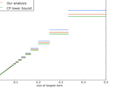
(a) A comparison of our analysis of $R_{SS}^{\infty}(\alpha)$ with Caprara and Pferschy’s (CP). The true ratio lies between the previously known upper and lower bounds.

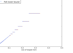
(b) Almost matching upper and lower bounds for the PoA of the parametric bin packing game.

	$R_{\mathit{FFD}}(\alpha)$ [13]	CP lb [3]	$R_{\mathit{SS}}(\alpha)$	CP ub [3]	$PoA(\alpha)$	$R_{\mathit{FF}}(\alpha)$ [13]
$t=1$	1.222222	1.606695 [10]	1.606695	1.621015	[1.641632, 1.642857] [8]	1.700000
$t=2$	1.183333	1.364307	1.376643	1.398793	[1.464571, 1.466667]	1.500000
$t=3$	1.166667	1.263293	1.273361	1.287682	[1.326180, 1.326530]	1.333333
$t=4$	1.150000	1.206935	1.214594	1.223143	[1.247771, 1.247863]	1.250000
$t=5$	1.138095	1.170745	1.176643	1.182321	[1.199102, 1.199134]	1.200000
$t=6$	1.119048	1.145460	1.150106	1.154150	[1.166239, 1.166253]	1.166667
$t=7$	1.109127	1.126763	1.130504	1.133531	[1.142629, 1.142635]	1.142857
$t=8$	1.097222	1.112360	1.115433	1.117783	[1.124867, 1.124871]	1.125000
$t=9$	1.089899	1.100918	1.103483	1.105360	[1.111029, 1.111031]	1.111111
$t=10$	1.081818	1.091603	1.093776	1.095310	[1.099946, 1.099947]	1.100000

(a) Comparison of the worst-case ratio of FFD, SS, FF and PoA as a function of $\alpha$ when $\alpha\leq\frac{1}{t}$, for $t=1,\ldots,10$.

Figure 1: Our results at a glance.

4 Concluding Remarks

In order to illustrate the results in the paper, we report in Figure 1(a) the values for the worst-case ratio of the SS algorithm for various values of $\alpha$ along with previously known upper and lower bounds of Caprara and Pferschy [3], and the worst-case approximation ratios of FF and FFD algorithm Bin Packing. We also include the range of possible values for the PoA for different values of $\alpha$. Figure 1(b) shows our (almost matching) upper and lower bound on the PoA. We conjecture that the true value of the $PoA$ equals our lower bound from Theorem 3.1.

small

Appendix A Omitted proofs

A.1 Proof of Lemma 2.2

Let $s$ be a solution to ($\mathrm{MP}_{r}$) other than $s^{*}$. The plan is to show that $s$ is not optimal by improving its cost. First we argue that without loss of generality $\sum_{i=1}^{r}s_{i}=1$. Indeed, if that was not the case then consider the new solution

$$s^{\prime}_{i}=\begin{cases}s_{i}&\text{if }i<r,\\ 1-\sum_{j=1}^{r-1}s_{j}&\text{if }i=r.\end{cases}$$

The difference between the value of $s^{\prime}$ and the value of $s$ comes from the $r$th term in the objective of ($\mathrm{MP}_{r}$). Since $s^{\prime}_{r}>s_{r}$, this difference is at least

$$s^{\prime}_{r}-\frac{s_{r}}{1-s^{\prime}_{r}+s_{r}}>s^{\prime}_{r}-\frac{s^{\prime}_{r}}{1-s^{\prime}_{r}+s^{\prime}_{r}}=0.$$

Let $i$ be the first index such that $s_{i}\neq s^{*}_{i}$. First, we consider the case $s_{i}<s^{*}_{i}$. Let $h>i$ be the smallest index such that $\sum_{j=1}^{h}s_{j}\geq 1-\min_{1\leq j\leq h}s_{j}$. (Note that such $h$ must exist because the condition is satisfied by $r$ and $i<r$ by our assumption that $\sum_{i}s_{i}=1$.) We construct a new solution $s^{\prime}$ from $s$ by slightly increasing $s_{i}$ and slightly decreasing $s_{h}$ by the same $\varepsilon$ amount (note that $s_{h}$ must be non-zero). We would like to argue that the overall change in value is positive. To that end, we examine how each term in the objective of ($\mathrm{MP}_{r}$) changes with the update.

• For $k\in[1,i)$ the contribution of the $k$th term is not affected by the update since its value does not depend on $s_{i}$ or $s_{h}$.

• For $k\in(i,h)$, the $k$th term can only increase. Indeed, for small enough $\varepsilon$ and for all $s^{\prime}_{i}\in[s_{i},\,s_{i}+\varepsilon]$ we have $\sum_{j=1}^{k}s^{\prime}_{j}<1-\min_{1\leq j\leq h}s^{\prime}_{j}$ and thus the contribution of the $k$th term to the value of $s^{\prime}$ is

  $$\frac{s^{\prime}_{k}}{1-\min_{1\leq j\leq k}s^{\prime}_{j}}\geq\frac{s_{k}}{1-\min_{1\leq j\leq k}s_{j}},$$

  which in turn is its contribution to the value of $s$.

• For $k\in(h,r]$, the $k$th term does not change with the update because, since $\sum_{j=1}^{k}s^{\prime}_{j}=\sum_{j=1}^{k}s_{j}$ and $\sum_{j=1}^{h}s_{j}\geq 1-\min_{1\leq j\leq h}s_{j}$, its contribution is always

  $$\frac{s_{k}}{\max\{\sum_{j=1}^{k}s_{k},\,1-\min_{h<j\leq k}s_{j}\}}.$$

• Regarding the $i$th term, for any $s^{\prime}_{i}\in[s_{i},s^{*}_{i}]$ we have $\sum_{j=1}^{i}s_{j}<1-\min_{1\leq j\leq i}s^{\prime}_{j}=1-s^{\prime}_{i}$. Thus its contribution to the value of $s$ is $\frac{s^{\prime}_{i}}{1-s^{\prime}_{i}}$. Imagine increasing $s^{\prime}_{i}$ continuously from $s_{i}$ to $s_{i}+\varepsilon$. The rate of change of its contribution to the value as a function of $s^{\prime}_{i}$ is

  $$\frac{\partial}{\partial x}\left(\frac{x}{1-x}\right)_{x=s^{\prime}_{i}}=\ \,\frac{1}{(1-s^{\prime}_{i})^{2}}.$$

• Since the $h$th term decreases with the update, we need to show that its rate of change, as we decrease $s^{\prime}_{h}$ from $s_{h}$ to $s_{h}-\varepsilon$, does not cancel out the rate of change of the $i$th term. Suppose $\sum_{j=1}^{h}s_{j}>1-s_{h}$ then its rate of change is

  $$-\,\frac{\partial}{\partial x}\left(\frac{x}{\sum_{j=1}^{h}s_{j}}\right)_{x=s^{\prime}_{h}}=\ -\,\frac{1}{\sum_{j=1}^{h}s_{j}}\geq-\,\frac{1}{1-s_{i}}>-\,\frac{1}{(1-s_{i})^{2}}.$$

  Let us consider what happens when $\sum_{j=1}^{h}s_{j}=1-s_{h}$. In this case $s_{h}\leq s_{i}$ since $1-s_{h}=\sum_{j=1}^{h}s_{j}\geq 1-\min_{1\leq j\leq h}s_{j}\geq 1-s_{i}.$ Thus, the rate of change of the $h$th term is

  $$-\,\frac{\partial}{\partial x}\left(\frac{x}{1-x}\right)_{x=s^{\prime}_{h}}=\ -\,\frac{1}{(1-s^{\prime}_{h})^{2}}\ \geq\ -\frac{1}{(1-s_{i})^{2}}.$$

We claim that for small enough $\varepsilon$, the value of $s^{\prime}$ must be strictly greater than the value of $s$. Indeed, by the discussion above, the overall change in value is at least

$$\int_{s_{i}}^{s_{i}+\varepsilon}\frac{1}{(1-s^{\prime}_{i})^{2}}-\frac{1}{(1-s_{i})^{2}}\ \mathrm{d}s^{\prime}_{i}>0.$$

Now let us see what happens when $s_{i}>s^{*}_{i}$. In this case we build our new solution $s^{\prime}$ by decreasing $s_{i}$ and increasing $s_{r}$ by the same infinitesimally small amount $\varepsilon$. As before, terms before the $i$th do not depend on $s_{i}$ or $s_{r}$ and therefore are not affected by the update. Since $s_{i}>\sum_{j=i+1}^{r}s_{j}>s_{i+1}$ we have $\min_{1\leq j\leq k}s^{\prime}_{j}=\min_{1\leq j\leq k}s_{j}$ for $k\in(i,r)$. Therefore, in this case, the $k$th term can only increase

$$\frac{s^{\prime}_{k}}{\max\{\sum_{j=1}^{k}s^{\prime}_{j},\,1-\min_{1\leq j\leq k}s^{\prime}_{j}\}}\geq\frac{s_{k}}{\max\{\sum_{j=1}^{k}s_{j},\,1-\min_{1\leq j\leq k}s_{j}\}}.$$

The $i$th term decreases and its rate of change is

$$-\,\frac{\partial}{\partial x}\left(\frac{x}{1-2^{-i+1}+x}\right)_{x=s_{i}}=\ -\,\frac{1-2^{-i+1}}{(1-2^{-i+1}+s_{i})^{2}}>-\,\frac{1-2^{-i+1}}{(1-2^{-i})^{2}}>-\,1.$$

On the other hand, the $r$th term increases and its rate of change is 1 due to our assumption that $\sum_{i}s_{i}=1$. Therefore, the overall rate of change of value is strictly positive.

A.2 Proof of Lemma 2.5

The plan is to show that given some solution $s$, either there exists $x\in\left[\frac{1}{t+1},\frac{1}{t}\right]$ such that the solution $s^{*}$ induced by $x$ equals $s$, or we can construct another solution $s^{\prime}$ that is closer to $s^{*}$ and has value at least as large as $s$. This process is repeated until we converge to $s^{*}$.

First, if $\sum_{j=1}^{r}s_{j}<1$ then we can safely increase $s_{r}$ to until the bin is full. Note that we can always do this because there is no upper bound on $s_{r}$. From now on we assume that $\sum_{j=1}^{r}s_{j}=1$.

Suppose there exists $s_{i}<\frac{1}{t+1}$ for some $i<t$ and let $i$ be the smallest such index. Let $h$ be the smallest index such that $\sum_{j=1}^{j}s_{j}\geq\max\{1-\min_{1\leq j\leq h}s_{j},\frac{t}{t+1}\}$. As was done in the proof of Lemma 2.2, we increase $s_{i}$ and decrease $s_{h}$ by the same $\varepsilon$ amount. The same argument used before shows that the value of $s^{\prime}$ is greater than the value of $s$. Therefore, we can assume that $s_{i}\geq\frac{1}{t+1}$ for all $i<t$. Under this assumption, each item contributes $s_{i}\frac{t}{t+1}$ to the objective, since

$$1-\min_{1\leq j\leq i}s_{i}\leq 1-\frac{1}{t+1}=\frac{t}{t+1}\text{ and }\sum_{1\leq j\leq i}s_{j}\leq\frac{t-1}{t}<\frac{t}{t+1}.$$

Setting $s^{\prime}_{i}=\frac{\sum_{1\leq j<t}s_{j}}{t-1}$ for each $i\in[t-1]$ does not affect the contribution of these items and can only increase the contribution of the remaining items since the transformation does not change the total size, but may increase the minimum size of the first $t-1$ items. Therefore, we can assume that $s_{1}=\cdots=s_{t-1}=x$ for some $x\in[\frac{1}{t+1},\frac{1}{t}]$.

At this point, we can apply the exact same argument as the one used in the proof of Lemma 2.2. For $i=t$ we note that if $s_{t}<s^{*}_{t}$ then for any $s^{\prime}_{i}\in[s_{i},s_{i}+\varepsilon]$ we have $1-s^{\prime}_{i}>1-\frac{1-x\,(t-1)}{2}\geq\frac{t}{t+1},$ where the last inequality uses $x\geq\frac{1}{t+1}$, and $1-s^{\prime}_{i}=1-2s^{\prime}_{i}+s^{\prime}_{i}>x\,(t-1)+s^{\prime}_{i}=\sum_{j=1}^{t}s^{\prime}_{i}.$ Therefore, the contribution of the $t$th term is $\frac{s^{\prime}_{t}}{1-s^{\prime}_{t}}$. Similarly, if $s_{t}>s^{*}_{t}$ then the contribution is $\frac{s^{\prime}_{t}}{\sum_{j=1}^{t}s^{\prime}_{j}}$. These are the properties needed to apply the argument used before. The conclusion is that for all $t\leq i<r$ the value of the program is maximized by setting $s_{i}$ to $\frac{1-\sum_{j=1}^{i-1}s_{j}}{2}$.

A.3 Proof of Lemma 2.6

Consider the variable change $y=\frac{1}{1-(t-1)x}$, which for $t\geq 2$ maps the range $[\frac{1}{t+1},\frac{1}{t}]$ for $x$ into the range $[\frac{t+1}{2},t]$ for $y$:

$$\lambda^{t}(x)=g(y)=(1-1/y)\frac{t+1}{t}+\sum_{i=1}^{\infty}\frac{1}{y\,2^{i}-1}.$$

This function and its derivative converge uniformly for $y$ in $[\frac{t+1}{2},t]$. Thus, the first derivative of $g$ can be obtained by term-wise differentiation

$$g^{\prime}(y)=\frac{t+1}{t\,y^{2}}-\sum_{i=1}^{\infty}\frac{2^{i}}{(y\,2^{i}-1)^{2}}=\frac{1}{y^{2}}\left(\frac{t+1}{t}-\sum_{i=1}^{\infty}\frac{2^{i}}{(2^{i}-1/y)^{2}}\right).$$

Notice that each term of the infinite sum, and thus the sum itself, is a decreasing function of $y$ for $y\geq 1$. It follows that either the sign of $g^{\prime}$ is the same throughout the interval $[\frac{t+1}{2},t]$ or it changes from negative to positive. In either case, the maximum must be attained at one of the ends of the interval. Hence, the maximum of $\lambda^{t}(x)$ in the domain $[\frac{1}{t+1},\frac{1}{t}]$ is attained either at $\frac{1}{t+1}$ or at $\frac{1}{t}$.

We claim that $\lambda^{t}(\frac{1}{t+1})>\lambda^{t}(\frac{1}{t})$ for all $t\geq 2$. Indeed, taking the difference of these two values we get

$$\lambda^{t}\left(\frac{1}{t+1}\right)-\lambda^{t}\left(\frac{1}{t}\right)=\frac{1}{t^{2}}-\sum_{i=1}^{\infty}\frac{1}{2^{i}\,t^{2}+(2^{i}-2)\,t-1+2^{-i}}$$

If the denominator of each term of the infinite sum were larger than $2^{i}t^{2}$ then it would immediately follow that the right hand side is always positive. Unfortunately, this is not true for the first term. Nevertheless, it is true for the remaining terms, and the first and second terms together are less than $\frac{3}{4t^{2}}$. Therefore,

$$\lambda^{t}\left(\frac{1}{t+1}\right)-\lambda^{t}\left(\frac{1}{t}\right)>\frac{1}{t^{2}}-\sum_{i=1}^{\infty}\frac{1}{2^{i}\,t^{2}}=0$$

A.4 Proof of Theorem 3.1

Let $s>2$ be an integer. We define a construction with $s+1$ phases of indices $0\leq j\leq s$, where the items of phase $j$ have sizes which are close to $\frac{1}{(t+1)\cdot 2^{j}}$, but can be slightly smaller or slightly larger than this value. We let $OPT=t(t-1)\cdot n+n$, and assume that $n$ is a large enough integer, such that $n>2^{s^{3}}$, $n>>t$. We use a sequence of small values, $\delta_{j}$ such that $\delta_{j}=\frac{1}{(4n)^{3s-2j}}$. Note that this implies $\delta_{j+1}=(4n)^{2}\delta_{j}$ for $0\leq j\leq s-1$. For each $t\geq 2$, $t\in\mathbb{N}$ we use two sequences of positive integers $r^{t}_{j}\leq n$ and $d^{t}_{j}\leq n$, for $2\leq j\leq s$, and in addition, $r^{t}_{0}=n$, $d^{t}_{0}=0$ and $r^{t}_{1}=\frac{n}{t+1}$, $d^{t}_{1}=\frac{t}{t+1}n$ (and thus $r^{t}_{1}+d^{t}_{1}=n$). We define $r^{t}_{j+1}=\frac{r^{t}_{j}-1}{(t+1)\cdot 2^{j-1}}$ and $d^{t}_{j+1}=r^{t}_{j}-r^{t}_{j+1}=\frac{((t+1)\cdot 2^{j-1}-1)r^{t}_{j}+1}{(t+1)\cdot 2^{j-1}}=((t+1)\cdot 2^{j-1}-1)r^{t}_{j+1}+1$, for $1\leq j\leq s-1$.

Observation A.1.

For each $1\leq j\leq s$, $\frac{n}{(t+1)^{j}\cdot 2^{j(j-1)/2}}-1\leq r^{t}_{j}\leq\frac{n}{(t+1)^{j}\cdot 2^{j(j-1)/2}}$.

Proof.

For $j=1$ it holds by definition. We next prove the property for $r^{t}_{j+1}$ using the definition of the sequence $r^{t}_{j}$. We have $r^{t}_{j+1}=\frac{r^{t}_{j}-1}{(t+1)\cdot 2^{j-1}}$ for $j\geq 1$. From this definition, we get (by induction) that

$$r^{t}_{j+1} =r^{t}_{1}\prod_{i=1}^{j}{\frac{1}{(t+1)\cdot 2^{i-1}}}-\sum_{i=1}^{j-1}{\frac{1}{(t+1)\cdot 2^{i}}}$$

$$=\frac{r^{t}_{1}}{(t+1)^{j}}\cdot\frac{1}{2^{j(j-1)/2}}-\frac{1}{t+1}(1-\frac{1}{2^{j-1}})$$

$$<\frac{n}{(t+1)^{j}\cdot 2^{j(j-1)/2}},$$

as $r^{t}_{1}<n$, and for $t\geq 2$ $\frac{1}{t+1}(1-\frac{1}{2^{j-1}})>0$. On the other hand, $\frac{1}{(t+1)^{j-1}\cdot 2^{j(j-1)/2}}\leq 1$ holds, since $(t+1)^{j-1}\cdot 2^{j(j-1)/2}\geq 1$ for $j\geq 1$. So $r^{t}_{j+1}\geq\frac{n}{(t+1)^{j}\cdot 2^{j(j-1)/2}}-1$. ∎

The input set of items for $t\geq 2$ consists of multiple phases. Phase 0 consists of the following sets of items; $nt$ items of size $\sigma_{01}=\frac{1}{t+1}+\Delta nt^{2}(t-1)+\Delta$, $t(t-1)n$ items of size $\sigma_{02}=\frac{1}{t+1}-\Delta nt(t-1)$, and pairs of items of sizes $\sigma^{i}_{03}=\frac{1}{t+1}+\Delta nt(t-1)+i\Delta$ and $\sigma^{i}_{04}=\frac{1}{t+1}-i\Delta$ for $1\leq i\leq t(t-1)n$, such that $\Delta=\frac{2\delta_{0}}{nt(t-1)+1}$. Note that $\sigma^{i}_{03}+\sigma^{i}_{04}=\frac{2}{t+1}+\Delta nt(t-1)$. There are also $(t-2)\cdot t(t-1)n$ items of size $\sigma_{05}=\frac{1}{t+1}$. For $1\leq j\leq s$, phase $j$ consists of the following $2d^{t}_{j}+r^{t}_{j}$ items. There are $r^{t}_{j}$ items of size $\sigma_{j}=\frac{1}{(t+1)\cdot 2^{j}}+2(d^{t}_{j}+1)\delta_{j}$, and for $1\leq i\leq d^{t}_{j}$, there are two items of sizes $\pi^{i}_{j}=\frac{1}{(t+1)\cdot 2^{j}}+(2i-1)\delta_{j}$ and $\theta^{i}_{j}=\frac{1}{(t+1)\cdot 2^{j}}-2i\delta_{j}$. Note that $\pi^{i}_{j}+\theta^{i}_{j}=\frac{1}{(t+1)\cdot 2^{j-1}}-\delta_{j}$. A bin of level $j$ in the optimal packing contains only items of phases $1,\ldots,j$. A bin of level $s+1$ contains items of all phases. The optimal packing contains $t(t-1)n$ bins of level 0, $d^{t}_{j}$ bins of level $j$, for $1\leq j\leq s$, and the remaining bins are of level $s+1$. Note that $\sum\limits_{j=1}^{s}d^{t}_{j}=\frac{t}{t+1}n+\sum\limits_{j=2}^{s}d^{t}_{j}=\frac{t}{t+1}n+r^{t}_{1}-r^{t}_{s}=\frac{t}{t+1}n+\frac{1}{t+1}n-r^{t}_{s}=n-r^{t}_{s}$. Thus, the number of level $s+1$ bins is (at most) $r^{t}_{s}$, and we have $n$ bins of levels $1\leq j\leq s+1$ allocated, in addition to the $t(t-1)n$ bins of level 0. In total, the packing contains of at most $t(t-1)n+n=(t(t-1)+1)n$ bins. The optimal packing of the set of items specified above is defined as follows. A level 0 bin contains $t-2$ items of size $\sigma_{05}$, one item of size $\sigma_{02}$ and, in addition, one pair of items of sizes $\sigma^{i}_{03}$ and $\sigma^{i}_{04}$ for a given value of $i$ such that $1\leq i\leq t(t-1)n$. For $1\leq j\leq s$, a level $j$ bin contains $t$ items of size $\sigma_{01}$ and one item of each size $\sigma_{k}$ for $1\leq k\leq j-1$, and, also, one pair of items of sizes $\pi^{i}_{j}$ and $\theta^{i}_{j}$ for a given value of $i$ such that $1\leq i\leq d^{t}_{j}$. A bin of level $s+1$ contains $t$ items of size $\sigma_{01}$ and one item of each size $\sigma_{k}$ for $1\leq k\leq s$.

Claim A.1.

This set of items can be packed into $n+t(t-1)n$ bins, i.e., $OPT\leq(1+t(t-1))n$

Proof.

First, we show that every item was assigned into some bin. Consider the $nt$ items of size $\sigma_{01}$. Each $t$-tuple of these items is assigned into a bin of level $1\leq j\leq s$ together. Consider items of size $\pi^{i}_{j}$ and $\theta^{i}_{j}$. Such items exist for $1\leq i\leq d^{t}_{j}$, therefore, every such pair is assigned into a bin (of level $1\leq j\leq s$) together. Next, consider items of size $\sigma_{j}$ for some $1\leq j\leq s$. The number of such items is $r^{t}_{j}$. The number of bins which received such items is $\sum\limits_{k=j+1}^{s}d^{t}_{k}+r^{t}_{s}=r^{t}_{j}$. As to the items of size $\sigma_{02}$. There are $t(t-1)n$ such items, each item is assigned into one of the $t(t-1)n$ bins of level 0. The items $\sigma^{i}_{03}$ and $\sigma^{i}_{04}$ that exist for $1\leq i\leq t(t-1)n$. Every such pair is assigned into one of the $t(t-1)n$ level 0 bins together. And, finally consider the $(t-2)\cdot t(t-1)n$ items of size $\sigma_{05}$. Each $(t-2)$ tuple of these items is assigned into one of the $t(t-1)n$ level 0 bins.

We further show that the sum of sizes of items in each bin does not exceed 1. Consider a bin of level 0. The sum of items it contains is: $(t-2)\sigma_{05}+\sigma_{02}+\sigma^{i}_{03}+\sigma^{i}_{04}=(t-2)\cdot\frac{1}{t+1}+\frac{1}{t+1}-\Delta nt(t-1)+\frac{2}{t+1}+\Delta nt(t-1)=1$. Now, consider a bin of level $j$ for some $1\leq j\leq s$. The sum of items packed in it is:

$$t\cdot\sigma_{01}+ \sum\limits_{k=1}^{j-1}\sigma_{k}+\frac{1}{(t+1)\cdot 2^{j-1}}-\delta_{j}$$

$$=t\cdot(\frac{1}{t+1}+\Delta nt^{2}(t-1)+\Delta)+\sum\limits_{k=1}^{j-1}(\frac{1}{(t+1)\cdot 2^{k}}+2(d^{t}_{k}+1)\delta_{k})+\frac{1}{(t+1)\cdot 2^{j-1}}-\delta_{j}$$

$$=\frac{t}{t+1}+t\cdot(\Delta nt^{2}(t-1)+\Delta)+\frac{1}{(t+1)\cdot 2^{j-1}}-\delta_{j}+\frac{1}{t+1}\sum\limits_{k=1}^{j-1}(\frac{1}{2^{k}}+2(d^{t}_{k}+1)\delta_{k})$$

$$=\frac{t}{t+1}+\frac{1}{(t+1)\cdot 2^{j-1}}+\frac{1-(\frac{1}{2})^{j-1}}{t+1}+t^{2}\cdot 2\delta_{0}-\delta_{j}+\sum\limits_{k=1}^{j-1}2(d^{t}_{k}+1)\delta_{k}$$

$$=1+t^{2}\cdot 2\delta_{0}+\sum\limits_{k=1}^{j-1}2(d^{t}_{k}+1)\delta_{k}-\delta_{j}.$$

It is left to show that $t^{2}\cdot 2\delta_{0}+\sum\limits_{k=1}^{j-1}2(d^{t}_{k}+1)\delta_{k}-\delta_{j}\leq 0$ holds. As $d_{k}+1\leq n$ and $\delta_{j}$ is a strictly increasing sequence, we have $2(d_{k}+1)\delta_{k}\leq 2n\delta_{j-1}$, and since $j-1\leq s<n$, $\sum\limits_{k=1}^{j-1}2(d_{k}+1)\delta_{k}<4n^{2}\delta_{j-1}$. Also, as $t<n$, $t^{2}\cdot 2\delta_{0}<2n^{2}\delta_{j-1}$. Using $\delta_{j}=16n^{2}\delta_{j-1}$ we get that the sum $t^{2}\cdot 2\delta_{0}+\sum\limits_{k=1}^{j-1}2(d^{t}_{k}+1)\delta_{k}$ is smaller than $\delta_{j}$.

It is left to consider a bin of level $s+1$. The sum of items in it is:

$$t\cdot\sigma_{01}+\sum\limits_{k=1}^{s}\sigma_{k} =t\cdot(\frac{1}{t+1}+\Delta nt^{2}(t-1)+\Delta)+\sum\limits_{k=1}^{s}(\frac{1}{(t+1)\cdot 2^{k}}+2(d^{t}_{k}+1)\delta_{k})$$

$$=\frac{t}{t+1}+t\cdot(\Delta nt^{2}(t-1)+\Delta)+\frac{1-(\frac{1}{2})^{s}}{(t+1)}+\sum\limits_{k=1}^{s}2(d_{k}+1)\delta_{k}$$

$$=1-\frac{(\frac{1}{2})^{s}}{(t+1)}+t\cdot 2\delta_{0}+\sum\limits_{k=1}^{s}2(d^{t}_{k}+1)\delta_{k}.$$

We have $2(d^{t}_{k}+1)\delta_{k}\leq 2n\delta_{s}=\frac{1}{2^{2s-1}n^{s-1}}$. Since $1<s<n$, $t<n$ and $t\cdot 2\delta_{0}<2n^{2}\delta_{s}$, we get that the quantity above is at most

$$1-\frac{(\frac{1}{2})^{s}}{(t+1)}+\frac{n}{2^{2s-1}n^{s-1}}+2n^{2}\delta_{s} =1-\frac{1}{2^{s}(t+1)}+\frac{1}{2^{2s-1}n^{s-2}}+2n^{2}\delta_{s}$$

$$=1-\frac{1}{2^{s}(t+1)}+\frac{1}{2^{2s-1}n^{s-2}}+\frac{2n^{2}}{(4n)^{s}}$$

$$=1-\frac{1}{2^{s}(t+1)}+\frac{1}{2^{2s-1}n^{s-2}}+\frac{1}{2^{2s-1}n^{s-2}}$$

$$=1-\frac{1}{2^{s}(t+1)}+\frac{1}{2^{2(s-1)}n^{s-2}}<1.$$

∎

Before introducing the NE packing for this set of items, we slightly modify the input by removing a small number of items. Clearly, $OPT\leq(1+t(t-1))n$ would still hold for the modified input. The modification applied to the input is a removal of items $\pi^{1}_{j}$ and $\theta^{d^{t}_{j}}_{j}$ for all $1\leq j\leq s$, the two items $\sigma^{1}_{03}$ and $\sigma^{t(t-1)n}_{04}$ and $(t-2)$ of the $\sigma_{05}$ items from the input. We now define an alternative packing, which is a NE. There are three types of bins in this packing. The bins of the first type are bins with items of phase $j$, $1\leq j\leq s+1$. We construct $r^{t}_{j}$ such bins. A bin of phase $j$ consists of $(t+1)\cdot 2^{j}-1$ items, as follows. One item of size $\sigma_{j}=\frac{1}{(t+1)\cdot 2^{j}}+2(d^{t}_{j}+1)\delta_{j}$, and $(t+1)\cdot 2^{j-1}-1$ pairs of items of phase $j$. A pair of items of phase $j$ is defined to be the items of sizes $\pi^{i+1}_{j}$ and $\theta^{i}_{j}$, for some $1\leq i\leq d^{t}_{j}-1$. The sum of sizes of this pair of items is $\frac{1}{(t+1)\cdot 2^{j}}+(2i+1)\delta_{j}+\frac{1}{(t+1)\cdot 2^{j}}-2i\delta_{j}=\frac{2}{(t+1)\cdot 2^{j}}+\delta_{j}=\frac{1}{(t+1)\cdot 2^{j-1}}+\delta_{j}$.

Using $d^{t}_{j}=((t+1)\cdot 2^{j-1}-1)r^{t}_{j}+1$ we get that all phase $j$ items, for $1\leq j\leq s$ are packed. The sum of items in every such bin is $1-\frac{1}{(t+1)\cdot 2^{j-1}}+((t+1)\cdot 2^{j-1}-1)\delta_{j}+\frac{1}{(t+1)\cdot 2^{j}}+2(d^{t}_{j}+1)\delta_{j}=1-\frac{1}{(t+1)\cdot 2^{j}}+\delta_{j}((t+1)\cdot 2^{j-1}+1+2d^{t}_{j})$.

The $nt$ bins of the second type in the NE packing contain $(t-1)$ items of size $\sigma_{02}=\frac{1}{t+1}-\Delta nt(t-1)$ and one item of size $\sigma_{01}=\frac{1}{t+1}+\Delta nt^{2}(t-1)+\Delta$, from the 0 phase bins. The load of each such bin is

$$(t-1)\left(\frac{1}{t+1}-\Delta nt(t-1)\right)+ \frac{1}{t+1}+\Delta nt^{2}(t-1)+\Delta$$

$$=\frac{t}{t+1}-\Delta nt(t-1)^{2}+\Delta nt^{2}(t-1)+\Delta$$

$$=\frac{t}{t+1}+\Delta nt(t-1)(t-(t-1))+\Delta$$

$$=\frac{t}{t+1}+\Delta nt(t-1)+\Delta$$

$$=\frac{t}{t+1}+\Delta(nt(t-1)+1)$$

$$=\frac{t}{t+1}+2\delta_{0},$$

by definition of $\Delta$. As there are in total $t(t-1)n$ identical items of size $\sigma_{02}$ and $nt$ identical $\sigma_{01}$ items in the input set, we get that all these items are packed in these $nt$ second type bins in the NE packing constructed above.

The $t(t-1)n-1$ bins of third type in the NE packing each contain $(t-2)$ items of size $\sigma_{05}=\frac{1}{t+1}$, and, in addition, one pair of items of sizes $\sigma^{i+1}_{03}$ and $\sigma^{i}_{04}$, for some $1\leq i\leq t(t-1)n$ from the phase 0 bins. The sum of sizes of this pair of items is: $\sigma^{i+1}_{03}+\sigma^{i}_{04}=\frac{1}{t+1}+\Delta nt(t-1)+(i+1)\Delta+\frac{1}{t+1}-i\Delta=\frac{2}{t+1}+\Delta(nt(t-1)+1)=\frac{2}{t+1}+2\delta_{0}$. Thus, the total load of such bin is $(t-2)\cdot\frac{1}{t+1}+\frac{2}{t+1}+2\delta_{0}=\frac{t}{t+1}+2\delta_{0}$, which equals the load of the bins of the second type in the NE packing. As there are in total $((t-2)\cdot t(t-1)n-(t-2))=(t-2)(t(t-1)n-1)$ items of size $\sigma_{05}$ and $t(t-1)n-1$ pairs of $\sigma^{i}_{03}$ and $\sigma^{i}_{04}$ items, we conclude that all the items of size $\sigma_{05}$ and $\sigma^{i}_{03}$, $\sigma^{i}_{04}$ are packed in these $t(t-1)n-1$ NE bins of the third type, as defined above.

We now should verify that the sum of sizes of the items packed in the three types of bins in the defined NE packing does not exceed 1. This holds for the second and the third type bins, as: $\frac{t}{t+1}+2\delta_{0}<\frac{t}{t+1}+2n\delta_{s}=\frac{t}{t+1}+\frac{2n}{(4n)^{s}}=\frac{t}{t+1}+\frac{1}{2^{2s-1}n^{s-1}}<\frac{t}{t+1}+\frac{1}{t+1}=1$. For the bins of the first type, this property directly follows from the inequality proven in the next claim.

Claim A.2.

The loads of the bins in the packing defined above are monotonically increasing as a function of the phase.

Proof.

It is enough to show $1-\frac{1}{(t+1)\cdot 2^{j}}+\delta_{j}((t+1)\cdot 2^{j-1}+1+2d^{t}_{j})<1-\frac{1}{(t+1)\cdot 2^{j+1}}$ for $1\leq j\leq s$, $t\geq 2$ which is equivalent to proving $\delta_{j}((t+1)\cdot 2^{j-1}+1+2d^{t}_{j})2^{j+1}<\frac{1}{t+1}$. Using $d^{t}_{j}<n$, we have: $\delta_{j}((t+1)\cdot 2^{j-1}+1+2d^{t}_{j})2^{j+1}<\delta_{j}((t+1)\cdot 2^{2j}+2^{j+2}n)<(t+1)\cdot 2\delta_{j}n^{2}$, as $n>2^{s^{3}}$. Using $\delta_{j}\leq\delta_{s}=\frac{1}{2^{2s}n^{s}}\leq\frac{1}{16n^{3}(t+1)^{2}}$ we get $2\delta_{j}n^{2}<\frac{1}{t+1}$.

For $j=0$, $\frac{t}{t+1}+2\delta_{0}<1-\frac{1}{(t+1)\cdot 2^{j}}+\delta_{j}((t+1)\cdot 2^{j-1}+1+2d^{t}_{j})$ holds for all $j\geq 1$, as $2\delta_{0}\leq\delta_{j}((t+1)\cdot 2^{j-1}+1+2d^{t}_{j})$, since $t\geq 2$ and $\delta_{j}$ is a strictly increasing sequence. ∎

Claim A.3.

The packing defined above is a valid NE packing.

Proof.

To show that this is a NE packing, we need to show the an item of phase $j>0$ cannot migrate to a bin of a level $k\geq j$, since this would result in a load larger than 1, and that it cannot migrate to a bin of phase $k<j$, since this would result in a load smaller than the load of a phase $j$ bin. Due to the monotonicity we proved in Claim A.2, we only need to consider a possible migration of a phase $j$ item into a phase $j$ bin, and a phase $j-1$ bin, if such bins exist. Moreover, in the first case it is enough to consider the minimum size item and in the second case, the maximum size item of phase $j$.

For phase 0 items, since the smallest phase 0 item has size $\frac{1}{t+1}-\Delta nt(t-1)$, if it migrates to another bin of this phase, we get a total load of $\frac{t}{t+1}+\Delta(nt(t-1)+1)+\frac{1}{t+1}-\Delta nt(t-1)=1+\Delta>1$, as $\Delta>0$.

For items of phase $j\geq 1$: The smallest phase $j$ item has size $\frac{1}{(t+1)\cdot 2^{j}}-\delta_{j}(2(d^{t}_{j}-1))=\frac{1}{(t+1)\cdot 2^{j}}-\delta_{j}(2d^{t}_{j}-2)$. If it migrates to another bin of this phase, we get a total load of

$$1-\frac{1}{(t+1)\cdot 2^{j}}+\delta_{j}( (t+1)\cdot 2^{j-1}+1+2d^{t}_{j})+\frac{1}{(t+1)\cdot 2^{j}}-\delta_{j}(2d^{t}_{j}-2)$$

$$=1+\delta_{j}((t+1)\cdot 2^{j-1}+1+2d^{t}_{j})-2d^{t}_{j}\delta_{j}+2\delta_{j}$$

$$=1+\delta_{j}(3+(t+1)\cdot 2^{j-1})>1.$$

The check for the largest item in the phase should be done separately for cases $j=1$ and $j\geq 2$, because we want to show that the largest item of phase $j=1$ (in first type bin) cannot migrate into a phase 0 bin (a second or third type bin), while for the largest item of phase $j\geq 2$ we need to show that it cannot move into other bin of first type. For phase $j=1$: The largest phase item has size $\frac{1}{2(t+1)}+2(d^{t}_{1}+1)\delta_{1}$. If it migrates to a bin of phase 0, we get a load of $\frac{t}{t+1}+2\delta_{0}+\frac{1}{2(t+1)}+2(d^{t}_{1}+1)\delta_{1}=\frac{2t+1}{2(t+1)}+2\delta_{0}+2(d^{t}_{1}+1)\delta_{1}$. This load is strictly smaller than a load of level $1$ which is $1-\frac{1}{(t+1)\cdot 2}+\delta_{1}((t+1)+1+2d^{t}_{1})=\frac{2t+1}{2(t+1)}+\delta_{1}((t+1)+1+2d^{t}_{1})$, as $t\geq 2$ and $\delta_{1}>\delta_{0}$.

For phase $j\geq 2$: The largest phase $j$ item has size $\frac{1}{(t+1)\cdot 2^{j}}+2(d^{t}_{j}+1)\delta_{j}$. If it migrates to a bin of phase $j-1$, we get a load of

$$1-\frac{1}{(t+1)\cdot 2^{j-1}}+\delta_{j-1} ((t+1)\cdot 2^{j-2}+1+2d^{t}_{j-1})+\frac{1}{(t+1)\cdot 2^{j}}+2(d^{t}_{j}+1)\delta_{j}$$

$$=1-\frac{1}{(t+1)\cdot 2^{j}}+\delta_{j-1}((t+1)\cdot 2^{j-2}+1+2d^{t}_{j-1})+2(d^{t}_{j}+1)\delta_{j}$$

$$=1-\frac{1}{(t+1)\cdot 2^{j}}+\delta_{j-1}((t+1)\cdot 2^{j-2}+1+2d^{t}_{j-1})+2d^{t}_{j}\delta_{j}+2\delta_{j}.$$

We compare this load with $1-\frac{1}{(t+1)\cdot 2^{j}}+\delta_{j}((t+1)\cdot 2^{j-1}+1+2d^{t}_{j})$, and prove that the first load is smaller. Indeed $\delta_{j-1}((t+1)\cdot 2^{j-2}+1+2d^{t}_{j-1})<\delta_{j}((t+1)\cdot 2^{j-1}-1)$ since $\delta_{j}=16n^{2}\delta_{j-1}$, $n>2^{s^{3}}$ and $((t+1)\cdot 2^{j-2}+1+2d^{t}_{j-1})<4n(t+1)<16n^{2}((t+1)\cdot 2^{j-1}-1)$. ∎

Finally, we bound the PoA as follows. The cost of the resulting NE packing is $nt+t(t-1)n-1+\sum\limits_{j=1}^{s}r^{t}_{j}=t^{2}n-1+\sum\limits_{j=1}^{s}r^{t}_{j}$. Using Observation A.1 we get that $\sum\limits_{j=1}^{s}r^{t}_{j}\geq\sum\limits_{j=1}^{s}(\frac{n}{(t+1)^{j}\cdot 2^{j(j-1)/2}}-1)$ and since $OPT=t(t-1)\cdot n+n$ and $n>>s$, we get a ratio of at least

$$\frac{t^{2}+\sum_{j=1}^{s}{(t+1)^{-j}\cdot 2^{-j(j-1)/2}}}{t(t-1)+1}.$$

Letting $s$ tend to infinity as well results in the claimed lower bound.

Note that we assume that all numbers $r^{t}_{j}$ and $d^{t}_{j}$ are integer values for each $t\geq 2$, which is not necessarily the case. To overcome this, we let $r^{t}_{j+1}=\big{\lfloor}\frac{r^{t}_{j}-1}{(t+1)\cdot 2^{j-1}}\big{\rfloor}$, for $0\leq j\leq s-1$, and $d^{t}_{j+1}=((t+1)\cdot 2^{j-1}-1)r^{t}_{j+1}+1$. In this case, it is possible to prove $\frac{n}{(t+1)^{j}\cdot 2^{j(j-1)/2}}-3\leq r^{t}_{j}\leq\frac{n}{(t+1)^{j}\cdot 2^{j(j-1)/2}}$, which leads to the same result.

A.5 Proof of Claim 3.1

Consider the well-known First Fit algorithm (FF for short) for bin packing. FF packs each item in turn into the lowest indexed bin to where it fits. It opens a new bin only in the case where the item does not fit into any existing bin. It was shown in [13] that any bin (accept for maybe two) in the packing produced by FF is more than $\frac{t}{t+1}$ full for any $t\geq 2$. For each $N_{G}$ instance, it is possible to define (modulo reordering the items) an instance for which running the FF algorithm will produce exactly the packing $b$. So, as any NE packing $b$ can be produced by a run of FF, it has all the properties of a FF packing, including the one mentioned above.

A.6 Proof of Claim 3.2

First, consider the bins in group $\mathcal{D}$. For $t\geq 3$, as all bins in $\mathcal{D}$ are filled by no more than $\frac{t^{2}-t+1}{t^{2}}$, no bin in this group (except maybe the leftmost bin) contains an item of size in $(0,\frac{t-1}{t^{2}}]$, as such an item will reduce its cost by moving to the leftmost bin in $\mathcal{D}$ (which is the bin with the largest load in $\mathcal{D}$), contradicting the fact that $b$ is an NE. Hence, all the items in bins (except for maybe one) in group $\mathcal{D}$ have items of sizes in $(\frac{t-1}{t^{2}},\frac{1}{t}]$. For $t=2$, as all bins in $\mathcal{D}$ are filled by no more than $\frac{17}{24}$, no bin in this group (except maybe the leftmost bin) contains an item of size in $(0,\frac{7}{24}]$, as such an item will reduce its cost by moving to the leftmost bin in $\mathcal{D}$, which contradicts the fact that $b$ is an NE. Hence, all the items in bins (except for maybe one) in group $\mathcal{D}$ have items of sizes in $(\frac{7}{24},\frac{1}{2}]$.

Now, consider the bins in group $\mathcal{C}$. For $t\geq 3$, as all bins in $\mathcal{C}$ are filled by no more than $\frac{t+1}{t+2}$, no bin in this group (except maybe the leftmost bin) contains an item of size in $(0,\frac{1}{t+2}]$, as such an item will reduce its cost by moving to the leftmost bin in $\mathcal{C}$ (which is the bin with the largest load in $\mathcal{C}$), contradicting the fact that $b$ is an NE. Also, no bin in $\mathcal{C}$ contains an item of size $x\in(\frac{1}{t+2},\frac{t-1}{t^{2}}]$, as such an item will benefit from moving to a bin in group $\mathcal{D}$, as $x+\frac{t}{t+1}>\frac{t+1}{t+2}$ for any $x>\frac{1}{(t+2)}$. Hence, all the items in bins in group $\mathcal{C}$ are of sizes in $(\frac{t-1}{t^{2}},\frac{1}{t}]$. For $t=2$, as all bins in $\mathcal{C}$ are filled by no more than $\frac{3}{4}$, no bin in this group (except maybe the leftmost bin) contains an item of size in $(0,\frac{1}{4}]$, as such an item will reduce its cost by moving to the leftmost bin in $\mathcal{D}$, which contradicts the fact that $b$ is an NE. Also, no bin in $\mathcal{C}$ contains an item of size $x\in(\frac{1}{4},\frac{7}{24}]$, as such an item will benefit from moving to a bin in group $\mathcal{D}$, as $x+\frac{2}{3}>\frac{3}{4}$ for any $x>\frac{1}{4}$. Hence, all the items in bins (except for maybe one) in group $\mathcal{C}$ have sizes in $(\frac{7}{24},\frac{1}{2}]$.

Finally, consider the bins in group $\mathcal{B}$. For $t\geq 3$, as all bins in $\mathcal{B}$ are filled by no more than $\frac{2t+1}{2(t+1)}$, no bin in this group (except maybe the leftmost bin) contains an item of size in $(0,\frac{1}{2(t+1)}]$, as such an item will reduce its cost by moving to the leftmost bin in $\mathcal{B}$ (which is the bin with the largest load in $\mathcal{B}$), contradicting the fact that $b$ is an NE. Also, no bin in $\mathcal{B}$ contains an item of size $x\in(\frac{1}{2(t+1)},\frac{t-1}{t^{2}}]$, as such an item will benefit from moving to a bin in group $\mathcal{D}$, as $x+\frac{t}{t+1}>\frac{2t+1}{2(t+1)}$ for any $x>\frac{1}{2(t+1)}$. Hence, all the items in bins (except for maybe one) in group $\mathcal{C}$ have items of sizes in $(\frac{t-1}{t^{2}},\frac{1}{t}]$. For $t=2$, as all bins in $\mathcal{B}$ are filled by no more than $\frac{5}{6}$, no bin in this group (except maybe the leftmost bin) contains an item of size in $(0,\frac{1}{6}]$, as such an item will reduce its cost by moving to the leftmost bin in $\mathcal{B}$, which contradicts the fact that $b$ is an NE. Also, no bin in $\mathcal{B}$ (except maybe the leftmost bin) contains an item of size $x\in(\frac{1}{6},\frac{7}{24}]$, as such an item will benefit from moving to a bin in group $\mathcal{D}$, as $x+\frac{2}{3}>\frac{5}{6}$ for any $x>\frac{1}{6}$. Hence, all the items in bins (except for maybe one) in group $\mathcal{C}$ have sizes in $(\frac{7}{24},\frac{1}{2}]$.

We conclude, that any bin in groups $\mathcal{B}$, $\mathcal{C}$ and $\mathcal{D}$, except for maybe a constant number of bins, contain only items of sizes in $(\frac{t-1}{t^{2}},\frac{1}{t}]$ for $t\geq 3$, and items of sizes in $(\frac{7}{24},\frac{1}{2}]$ for $t=2$.

Now, we show that each one of these bins contains exactly $t$ such items. Note, that by definition of the groups all bins in $\mathcal{B}$, $\mathcal{C}$ and $\mathcal{D}$ (except maybe two) have loads in $(\frac{t}{t+1},\frac{2t+1}{2(t+1)}]$ for $t\geq 3$, or in $(\frac{2}{3},\frac{5}{6}]$ for $t=2$.

If a bin contains at most $t-1$ such items, then it has a load of at most $(t-1)\cdot\frac{1}{t}=\frac{t-1}{t}$ for $t\geq 3$ of at most $\frac{7}{24}$ for $t=2$, which is less than the assumed load in these bins, so they must have more than $(t-1)$ such items.

If a bin contains at least $t+1$ such items, then it has a load of at least $(t+1)\cdot\frac{t-1}{t^{2}}=1-\frac{1}{t^{2}}$, which is greater than $\frac{2t+1}{2(t+1)}$ for $t\geq 3$, or at least $\frac{7}{8}$ which is greater than $\frac{5}{6}$ for $t=2$, so they must have less than $(t+1)$ such items.

We conclude that each bin in groups $\mathcal{B}$, $\mathcal{C}$ and $\mathcal{D}$), except for maybe 5 special bins (the leftmost bins in groups $\mathcal{B}$, $\mathcal{C}$ and $\mathcal{D}$ and the two rightmost bins in $\mathcal{D}$) contain exactly $t$ items with sizes in $(\frac{t-1}{t^{2}},\frac{1}{t}]$ for $t\geq 3$, or exactly $2$ items of sizes in $(\frac{7}{24},\frac{1}{2}]$ for $t=2$.

A.7 Proof of Claim 3.3

Assume by contradiction that $(N_{t}+k)\cdot t$ of these items for $k\geq 0$ are packed together in $t$-tuples in bins of groups $\mathcal{B}$, $\mathcal{C}$ and $\mathcal{D}$ in the $NE$ packing. Consider the first $N_{t}$ such bins. Call them $B_{1},B_{2},\ldots,B_{N_{t}}$. In a slight abuse of notation, we use $B_{i}$ to indicate both the $i$-th bin and its load. Denote the sizes of the remaining $N_{t}$ $t$-items by $t_{1},t_{2},\ldots,t_{N_{t}}$. These items are also packed in bins of groups $\mathcal{B}$, $\mathcal{C}$ and $\mathcal{D}$ in $b$, and share their bin with $t-1$ $t$-items (when at least one of these items is not packed in any of the aforementioned $N_{t}$ bins in the optimal packing). Obviously, as all these $N_{t}\cdot(t+1)$ $t$-items fit into $N_{t}$ unit-capacity bins, $t_{1}+\ldots+t_{N_{t}}+B_{1}+\ldots+B_{N_{t}}\leq N_{t}$ holds. To derive a contradiction, we use the following observation:

Observation A.2.

A $t$-tuple of items with sizes in $(\frac{t-1}{t^{2}},\frac{1}{t}]$ always has a greater total size than any $(t-1)$-tuple of such items.

Proof.

The total size of any $(t-1)$ items with sizes in $(\frac{t-1}{t^{2}},\frac{1}{t}]$ is at most $\frac{t-1}{t}$, while the total size of any $t$ items with sizes in $(\frac{t-1}{t^{2}},\frac{1}{t}]$ is strictly greater than $\frac{t(t-1)}{t^{2}}=\frac{t-1}{t}$. ∎

Thus, any item $t_{i}$, $1\leq i\leq N_{t}$ would be better off sharing a bin with other $t$ items of size in $(\frac{t-1}{t^{2}},\frac{1}{t}]$ instead of just $t-1$ such items as it does in the $NE$ packing $b$. For an item which shares a bin with $t-1$ $t$-items we conclude that the only reason it does not move to another bin with $t$ such items in $b$ is that it does not fit there.

So, we know that no item $t_{1}$, $1\leq i\leq N_{t}$ fits in any of the bins $B_{1},B_{2},\ldots,B_{N_{t}}$ in $b$. We get that for any $1\leq i\leq N_{t}$, for any $1\leq j\leq N_{t}$, the inequality $t_{i}+B_{j}>1$ holds. Summing these inequalities over all $1\leq i\leq N_{t}$ and $1\leq j\leq N_{t}$ we get $t_{1}+\ldots+t_{N_{t}}+B_{1}+\ldots+B_{N_{t}}>N_{t}$, which is a contradiction.

References

- [1] N. Andelman, M. Feldman, and Y. Mansour. Strong price of anarchy. In SODA, pages 189–198, 2007.
- [2] V. Bilò. On the packing of selfish items. In IPDPS. IEEE, 2006.
- [3] A. Caprara and U. Pferschy. Worst-case analysis of the subset sum algorithm for bin packing. Oper. Res. Lett., 32(2):159–166, 2004.
- [4] E. G. Coffman Jr. and J. Csirik. Performance guarantees for one-dimensional bin packing. In T. F. Gonzalez, editor, Handbook of Approximation Algorithms and Metaheuristics, chapter 32. Chapman & Hall/Crc, 2007. 18 pages.
- [5] E. G. Coffman, Jr., M. R. Garey, and D. S. Johnson. Approximation algorithms for bin packing: A survey. In D. S. Hochbaum, editor, Approximation algorithms. PWS Publishing Company, 1997.
- [6] J. Csirik and J. Y.-T. Leung. Variants of classical one-dimensional bin packing. In T. F. Gonzalez, editor, Handbook of Approximation Algorithms and Metaheuristics, chapter 33. Chapman & Hall/Crc, 2007. 13 pages.
- [7] A. Czumaj and B. Vöcking. Tight bounds for worst-case equilibria. ACM Transactions on Algorithms, 3(1), 2007.
- [8] L. Epstein and E. Kleiman. Selfish bin packing. In ESA, pages 368–380, 2008.
- [9] A. Fiat, H. Kaplan, M. Levy, and S. Olonetsky. Strong price of anarchy for machine load balancing. In ICALP2007, pages 583–594, 2007.
- [10] R. L. Graham. Bounds on multiprocessing anomalies and related packing algorithms. In Proceedings of the 1972 Spring Joint Computer Conference, pages 205 –217, 1972.
- [11] N. Immorlica, M. Mahdian, and V. S. Mirrokni. Cycle cover with short cycles. In Proceedings of the 22th Annual Symposium on Theoretical Aspects of Computer Science, pages 641–653, 2005.
- [12] K. Jain, M. Mahdian, E. Markakis, A. Saberi, and V. V. Vazirani. Greedy facility location algorithms analyzed using dual fitting with factor-revealing LP. Journal of the ACM, 50(6):795–824, 2003.
- [13] D. S. Johnson, A. J. Demers, J. D. Ullman, M. R. Garey, and R. L. Graham. Worst-case performance bounds for simple one-dimensional packing algorithms. SIAM J. Comput., 3(4):299–325, 1974.
- [14] E. Koutsoupias and C. H. Papadimitriou. Worst-case equilibria. In STACS’99, pages 404–413, 1999.
- [15] C. C. Lee and D. T. Lee. A simple online bin packing algorithm. J. ACM, 32:562–572, 1985.
- [16] M. Mavronicolas and P. G. Spirakis. The price of selfish routing. In STOC2001, pages 510–519, 2001.
- [17] T. Roughgarden. Selfish routing and the price of anarchy. MIT Press, 2005.
- [18] T.Roughgarden and É. Tardos. How bad is selfish routing? In FOCS, pages 93–102, 2000.
- [19] J. D. Ullman. The performance of a memory allocation algorithm. Technical Report 100, Princeton University, Princeton, NJ, 1971.
- [20] G. Y. and G. Zhang. Bin packing of selfish items. In WINE, pages 446–453, 2008.