Random graph models for directed acyclic networks

Abstract

We study random graph models for directed acyclic graphs, an important class of networks that includes citation networks, food webs, and feed-forward neural networks among others. We propose two specific models, roughly analogous to the fixed edge number and fixed edge probability variants of traditional undirected random graphs. We calculate a number of properties of these models, including particularly the probability of connection between a given pair of vertices, and compare the results with real-world acyclic network data finding that theory and measurements agree surprisingly well—far better than the often poor agreement of other random graph models with their corresponding real-world networks.

I Introduction

A directed acyclic graph is a directed graph with no cycles—closed paths across the graph that start and end at the same vertex and follow edges only in their forward direction. Directed acyclic graphs are a fundamental class of networks that occur widely in natural and man-made settings. The best-studied examples are citation networks, networks in which the vertices represent documents and the directed edges represent citations between them. Citation networks of learned papers have long been an object of study in the information sciences Price (1965); Egghe and Rousseau (1990); Seglen (1992) and more recently in physics Redner (1998); Lehmann et al. (2003), and citation networks of patents Jaffe and Trajtenberg (2002) and legal cases Fowler et al. (in press); Leicht et al. (2007) have also received some attention in the last few years. Directed acyclic graphs occur in many other areas too. In biology, phylogenetic networks representing gene transfer are strictly acyclic and food webs are approximately so. In computer science and engineering acyclic or approximately acyclic graphs occur in data structures, software call graphs, and feed-forward neural networks. In pure mathematics acyclic graphs are studied for their own sake Pittel and Tungol (2001); Barak and Erdős (1984); McKay et al. (2004) and as a representation of partially ordered sets Łuczak (1991) and random graph orders Albert and Frieze (1989); Bollobás and Brightwell (1997), while in statistics the widely used Bayesian networks are an acyclic graph version of probabilistic graphical models Jensen (2001); Ide and Cozman (2002); Mengshoel et al. (2006).

Over the years, the study of networks has been substantially illuminated by the development of random graph models. Such models include the original (Poisson) random graph famously studied by Erdős and Rényi Erdős and Rényi (1959, 1960), the configuration model of Molloy and Reed and others Bollobás (1980); Łuczak (1992); Molloy and Reed (1995, 1998) and its generalizations to directed, bipartite, and other network types Newman et al. (2001); Dorogovtsev et al. (2001), the small-world model of Watts and Strogatz Watts and Strogatz (1998), exponential random graphs Holland and Leinhardt (1981); Strauss (1986), and others. These models, combining simple definitions with complex but still analytically accessible structures, have provided an invaluable window on the expected behavior of large networks, as well as serving as the starting point for many other more sophisticated models and calculations.

To the best of our knowledge, however, no corresponding model has been studied for directed acyclic graphs—no equivalent of the configuration model for networks such as citation networks or food webs. In this paper, we propose such a model and study its properties in detail, giving derivations of a variety of quantities of interest, extensive numerical simulations, and comparisons with the behavior of real-world acyclic graphs, with which, in some cases, the model appears to be in surprisingly good agreement. A brief report of some of the material in this paper has appeared previously as Ref. Karrer and Newman (2009).

II Acyclic graphs and ordered graphs

To correctly specify a random graph model for directed acyclic graphs it is crucial first to understand the reason why such graphs are acyclic in real life. In most practical examples the acyclic nature of the network arises because the vertices are ordered. In citation networks and phylogenetic networks, for example, the vertices are time ordered: academic papers have a date or time of publication; species have a time of origination or speciation. In food webs vertices are ordered according to tropic level. (Trophic level, however, is often only an approximate concept and not precisely defined, which is why some food webs are only approximately acyclic, containing a few violations of the no-loops condition.) In software call graphs, the vertices, representing functions or subroutines, are ordered according to the software abstraction layer they occupy, and so forth.

In each of these cases, it is the ordering of the vertices and not their acyclic structure that is the definitive property of the network. The acyclic structure is merely a corollary of the ordering. In citation networks, for instance, papers can only cite others that came before them in time, and this eliminates closed cycles because all paths in the network must lead backward in time and there are no forward paths available to close the cycle. Similarly in food webs species of higher trophic level prey on those of lower level. In software graphs functions at higher levels of abstraction call those at lower levels. The name “directed acyclic graph” is thus perhaps slightly misleading, focusing our attention, as it does, on the acyclic property rather than the more fundamental ordering. A better name might be “directed ordered graphs,” but unfortunately the literature on this topic has long ago settled on the older name and it seems unwise to try and change it now.

What is important for our purposes, however, is that a sensible random graph model for these networks should mirror the features seen in the real world and incorporate an underlying ordering of the vertices that then drives the acyclic structure. Thus the correct model is really a “random ordered graph” and this is the approach we take in this paper note1 .

III Random directed acyclic graphs with fixed degree sequences

In this paper we propose two related random graph models of directed acyclic graphs. The two models are roughly analogous to the well known $G(n,m)$ and $G(n,p)$ versions of the standard Poisson random graph Erdős and Rényi (1959), one fixing the number of edges in the network exactly and the other fixing only the expected number. We begin by describing the “$G(n,m)$” version, which we introduced previously in Ref. Karrer and Newman (2009). The “$G(n,p)$” version, which is introduced for the first time in this paper, is described in Section IV.

Our first model takes as its input an ordered degree sequence consisting of the in-degree $k^{\mathrm{in}}_{i}$ and out-degree $k^{\mathrm{out}}_{i}$ for each vertex $i=1\ldots n$, where $n$ is the total number of vertices in the network. The directed edges in the model are allowed to run only from vertices with higher indices to vertices with lower, and this constraint enforces the acyclic nature of the network. Thus we can have an edge running to vertex $i$ from vertex $j$ only if $i<j$.

Throughout this paper we describe our networks in the language of time ordering: vertices are “earlier” or “later” in the network, meaning they have lower or higher indices, and the vertices with the lowest and highest indices are referred to as “first” and “last.” The use of these terms is purely for convenience and should not be taken as restricting the model to networks in which the vertices are time ordered. The concepts we introduce can be applied equally to networks such as food webs and call graphs in which the ordering has nothing to do with time.

III.1 Graphical degree sequences

A first important point to notice is that not all degree sequences are realizable as ordered acyclic graphs of the type described here. By analogy with similar issues in other branches of graph theory, we will refer to realizable degree sequences as graphical.

As with all directed graphs, if a degree sequence is to be graphical the sum of the in-degrees of all vertices must equal the sum of the out-degrees, since every edge that starts somewhere ends somewhere. Both sums are also individually equal to the total number $m$ of edges in the network:

$$\sum_{i=1}^{n}k^{\mathrm{in}}_{i}=\sum_{i=1}^{n}k^{\mathrm{out}}_{i}=m.$$ (1)

For a directed acyclic graph, however, there are also additional conditions. For instance, the first ($i=1$) vertex in the graph can never have any outgoing edges, since there are no earlier vertices for such edges to attach to. Thus $k^{\mathrm{out}}_{1}=0$ always in a graphical degree sequence. Similarly $k^{\mathrm{in}}_{n}=0$. More generally, we can derive a condition on the out-degree of every vertex as follows.

It is helpful to visualize in- and out-degrees as sets of “stubs” of edges pointing in and out of each vertex in the appropriate numbers. To create a complete network we need to match the stubs in pairs, out with in, to make whole edges, and a degree sequence is graphical only if all stubs can be matched while respecting the ordering of the vertices.

The number of stubs outgoing from vertices below vertex $i$ is $\sum_{j=1}^{i-1}k^{\mathrm{out}}_{j}$ and each such stub must be matched with an ingoing stub at a vertex below $i$, of which there $\sum_{j=1}^{i-1}k^{\mathrm{in}}_{j}$. The number of ingoing stubs below $i$ that are left over after we do this matching is

$$\mu_{i}=\sum_{j=1}^{i-1}k^{\mathrm{in}}_{j}-\sum_{j=1}^{i-1}k^{\mathrm{out}}_{j}.$$ (2)

This is the number of ingoing stubs below vertex $i$ that are available to attach to outgoing stubs at $i$ and above. Note that this number is determined entirely by the degree sequence—it does not depend on any of the details of which vertices are connected to which others.

Now consider vertex $i$ itself. Its out-degree $k^{\mathrm{out}}_{i}$ is the number of its outgoing stubs, and each of those stubs must be matched with an ingoing one below $i$. That means that $k^{\mathrm{out}}_{i}$ cannot be greater than $\mu_{i}$ above—if it were, then there would not be enough in-stubs available for $i$’s out-stubs to attach to and the degree sequence would not be graphical. Thus a necessary condition for a degree sequence to be graphical is

$$k^{\mathrm{out}}_{i}\leq\sum_{j=1}^{i-1}k^{\mathrm{in}}_{j}-\sum_{j=1}^{i-1}k^{\mathrm{out}}_{j}.$$ (3)

For convenience, we define

$$\lambda_{i}=\sum_{j=1}^{i-1}k^{\mathrm{in}}_{j}-\sum_{j=1}^{i}k^{\mathrm{out}}_{j},$$ (4)

so that (3) can be written as

$$\lambda_{i}\geq 0.$$ (5)

This condition must hold for all $i$ if the degree sequence is to be graphical.

Our earlier condition that $k^{\mathrm{out}}_{1}=0$ trivially implies that $\lambda_{1}=0$, and $k^{\mathrm{in}}_{n}=0$ implies that $\lambda_{n}=0$ because

$$\lambda_{n} =\sum_{j=1}^{n-1}k^{\mathrm{in}}_{j}-\sum_{j=1}^{n}k^{\mathrm{out}}_{j}$$

$$=(m-k^{\mathrm{in}}_{n})-m=0,$$ (6)

where we have made use of Eq. (1). Thus we also have

$$\lambda_{1}=\lambda_{n}=0.$$ (7)

One might imagine that one could now make a similar argument about the in-degrees of each vertex and derive a second condition for graphical sequences of the form:

$$\sum_{j=i+1}^{n}k^{\mathrm{out}}_{j}-\sum_{j=i}^{n}k^{\mathrm{in}}_{j}\geq 0.$$ (8)

This is correct, but in fact it is just another form of the first condition, Eq. (5), as the reader can easily verify by applying Eq. (1).

Equations (5) and (7) are a necessary condition for the degree sequence to be graphical. It’s straightforward to show that they are also sufficient. The proof is a constructive one: we build a network starting from the first vertex and working up. If (5) holds then at each vertex $i$ we know that the number of free in-stubs at lower vertices is at least $k^{\mathrm{out}}_{i}$, and hence there are in-stubs available to attach all of our out-stubs to. If we simply choose between the available stubs in any way we like, create the appropriate edges, and move on to the next vertex, then so long as there are no unused in-stubs left when we get to the last vertex, which is guaranteed by Eq. (7), we will have built a complete graph and hence the sequence is graphical.

Thus Eqs. (5) and (7) are a necessary and sufficient condition for a graphical degree sequence.

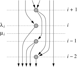
Figure 1: The flux $\mu_{i}$ is equal to the number of edges from vertices $i$ and above that connect to vertices below $i$. The excess flux $\lambda_{i}$ is the number of edges that go around vertex $i$, connecting vertices above to vertices below without passing through $i$. In this example $\mu_{i}=6$ and $\lambda_{i}=5$.

The quantities $\mu_{i}$ and $\lambda_{i}$ have a simple geometric interpretation as shown in Fig. 1. If we make a cut in our graph between vertices $i$ and $i-1$, the quantity $\mu_{i}$ is the number of edges that cross the cut, or the number flowing from higher to lower vertices. For this reason, we call $\mu_{i}$ the flux at vertex $i$. (Technically the flux is a property not of the vertex but of the gap between vertices $i$ and $i-1$, but we have to give it a label so we choose to label it with the upper of the two vertices.)

The quantity $\lambda_{i}$ is equal to the number of edges that flow “around” vertex $i$, meaning the number that run from vertices above $i$ to vertices below. We call this quantity the excess flux at vertex $i$. Using Eq. (2), we can show that the flux and excess flux are related by

$$\mu_{i}=\lambda_{i}+k^{\mathrm{out}}_{i}=\lambda_{i-1}+k^{\mathrm{in}}_{i-1}.$$ (9)

In the limit of large network size, as we will shortly see, the flux and excess flux are equal to one another to within a fraction of order $1/n$, and we will refer to both simply as “flux” in this limit.

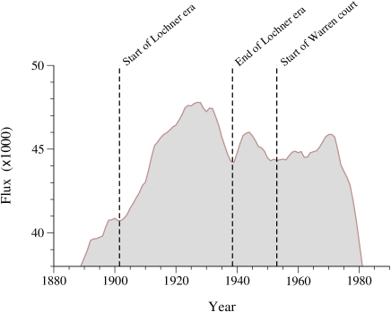
Figure 2: Flux $\mu_{i}$ for the network of citations between legal opinions of the US Supreme Court, plotted as a function of year of publication. The three dotted lines highlight dips in the flux and correspond roughly to three widely acknowledged shifts in the legal philosophy of the court: the start and end of the “Lochner era,” during which the court took a strong anti-regulatory stance, and the start of the Warren court. (Note that the origin is suppressed on the vertical axis.)

The flux is a quantity of interest in its own right in real-world networks. Low values of flux indicate “bottlenecks” in a network—lines across which few edges flow—and high values indicate regions in which there are many edges. Figure 2, for example, shows the measured flux as a function of time for the network of citations between legal decisions of the Supreme Court of the United States Leicht et al. (2007). A number of dips in the flux are visible in the figure (marked with dotted lines). In legal terms, these dips correspond to temporal divisions between sets of opinions such that the earlier set is little cited by the later set. It is a reasonable guess that these divisions reflect changes in legal thought that made older opinions obsolete, and indeed each of the three dips highlighted in the figure corresponds to an acknowledged shift in Supreme Court jurisprudence, as indicated.

III.2 Definition of the model

The definition of our random graph model is now straightforward. In the language of “stubs” introduced above, a graph on a graphical degree sequence is created by matching in- and out-going stubs in pairs to create $m$ complete edges while respecting the ordering of the vertices (meaning that out-stubs can connect only to earlier in-stubs). Our model is defined to be the ensemble of all such matchings in which every matching appears with equal probability.

This definition is the exact equivalent for directed acyclic graphs of the standard configuration model for undirected graphs Molloy and Reed (1995). In the configuration model one matches undirected stubs in pairs to create undirected edges and all matchings appear with equal probability in the ensemble. Note that in our model, as in the configuration model, multiedges are allowed. That is, the same pair of vertices can be connected by more than one edge. (Unlike the configuration model, there are no self-edges in an acyclic network, since this would violate the no-cycles rule.) Multiedges occur in some real-world acyclic networks, but not in others. In the model, however, they typically constitute a small $\mathrm{O}(1/n)$ fraction of all edges, and so are negligible in the large system size limit. At the same time, a model that admits them is far easier to study analytically than a model that does not.

Note also that the model includes random ordered trees—which have been widely studied in the past—as a special case. If every vertex in the network (other than the first) has out-degree 1 then the network is necessarily a tree and the ensemble is uniform over all ordered tree-like matchings with the given degrees.

Although the model is simple and intuitive, there are—just as with the configuration model—some subtleties to its definition. An important point to notice is that matchings of stubs are not in one-to-one correspondence with network topologies. Imagine our stubs to be labeled somehow, with letters or numbers, so that each one is uniquely identifiable. There will then, in general, be many different matchings that correspond to each possible network topology. If we take a matching and simply permute the labels of the out-stubs at a single vertex $i$, we produce a new matching corresponding to the same topology. The number of distinct such permutations is $k^{\mathrm{out}}_{i}!$. We can similarly permute the in-stubs at vertex $i$ for a total of $k^{\mathrm{in}}_{i}!$ permutations, and the number of permutations of all stubs at all vertices is then $\prod_{i}k^{\mathrm{in}}_{i}!k^{\mathrm{out}}_{i}!$. This, in the simplest case, is the number of matchings that correspond to each topology. Since this number is a function solely of the degree sequence, it is the same for all topologies, and hence if all matchings occur with equal probability $p$, then all topologies occur with equal probability $p\prod_{i}k^{\mathrm{in}}_{i}!k^{\mathrm{out}}_{i}!$.

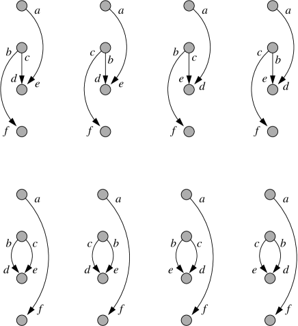
Figure 3: Top: a small directed acyclic network with four vertices and three edges. The stubs at each vertex are labeled with letters, and the four versions of the graph show the matchings of the stubs generated by permuting the stubs at each vertex. Each permutation generates a different matching, so there are in this case four matchings corresponding to the same graph, as we would expect since the product $\prod_{i}k^{\mathrm{in}}_{i}!k^{\mathrm{out}}_{i}!=4$ in this case. Bottom: a second graph with the same degree sequence, but now with a multiedge between the two center vertices. There are again four permutations of the stubs as shown, but now they correspond to only two different matchings—close inspection reveals that the first and fourth matchings are the same, as are the second and third. Thus in this case there are only two matchings for this graph. If all matchings are generated with equal probability, as in our model, then the top graph will be generated twice as often as the bottom one.

Unfortunately, there is a complication: if there are multiedges in the graph then the argument breaks down. Figure 3 shows why. If we identically permute the in-stubs at one end of a multiedge and the out-stubs at the other end, then we do not generate a new matching—we get back the same matching we started with. We see this effect in the lower half of the figure, where the four distinct permutations of stubs generate only two distinct matchings. (The top half of the figure shows another graph with the same degree sequence but no multiedges and in this case each permutation generates a unique matching.)

The net result is that our previous calculation overcounts the number of matchings per topology by a factor of the number of permutations of edges within multiedges. If there are no multiedges, then our previous calculation is correct. If there are multiedges then the number of matchings is reduced by a factor of $\prod_{i<j}A_{ij}!$, where $A_{ij}$ is an element of the adjacency matrix, i.e., the number of edges between vertices $i$ and $j$. Since this factor depends on the number and multiplicity of the multiedges, it follows that in general all topologies are not sampled with exactly equal probability in our model.

In practice, this is not a significant problem. The same issue arises in the configuration model but does not reduce the usefulness of that model. For the sake of precision, however, we note that although our model samples matchings with equal probability, it samples topologies with unequal probabilities that depend on the number and multiplicity of multiedges.

III.3 Computer generation of networks

One attractive feature of the model proposed here is that it is straightforward to generate networks drawn from the model’s ensemble on a computer. Previous methods for generating directed acyclic graphs have relied on Monte Carlo techniques Ide and Cozman (2002); Melancon et al. (2001); Mengshoel et al. (2006) but these methods, while versatile, are quite slow. Our model, by contrast, allows us to generate networks rapidly, in time $\mathrm{O}(m)$, where $m$ again is the total number of edges in the network. The algorithm, described briefly in Karrer and Newman (2009), is based on the scheme outlined in Section III.1 for building a network. Starting with $n$ vertices and an appropriate number of stubs at each, we go through the vertices in order from 1 to $n$. For each vertex we randomly join its outgoing stubs to ingoing ones at lower vertices chosen uniformly from the set of all such in-stubs that are currently unused. When all stubs have been matched in this fashion, the network is complete and the algorithm ends.

It is straightforward to see that indeed this algorithm generates all matchings with equal probability. Consider the step of the algorithm at which out-stubs from vertex $i$ are matched to suitable in-stubs. The number of out-stubs is $k^{\mathrm{out}}_{i}$ and the number of in-stubs available to match them to is, by definition, equal to the flux $\mu_{i}$. Thus the number of different matchings of stubs on this $i$th step is $N_{i}=\mu_{i}!/(\mu_{i}-k^{\mathrm{out}}_{i})!=\mu_{i}!/\lambda_{i}!$, where we have used Eq. (9) in the second equality, and the algorithm chooses between these uniformly at random so that each one occurs with equal probability $1/N_{i}$. Repeating the process for all $n$ vertices generates a unique matching of the entire graph with probability

$$\prod_{i=2}^{n}\frac{1}{N_{i}}=\prod_{i=2}^{n}{\lambda_{i}!\over\mu_{i}!}.$$ (10)

This probability is clearly uniform over all possible matchings since it depends only on the degree distribution and not on any details of the matching itself.

The algorithm can be implemented efficiently by maintaining in an ordinary array a list of currently unclaimed in-stubs from which we choose at random on every step. As soon as it is chosen, each stub is erased from the list by moving the list’s last item into its place. The operations for each stub can be performed in time $\mathrm{O}(1)$, and hence the total running time is simply proportional to the total number of in-stubs, which is $m$.

III.4 Expected number of edges

One of the most fundamental properties of our model is the expected number of directed edges between any two vertices $i$ and $j$. We will denote this quantity $P_{ij}$. In the limit of large network size $P_{ij}$ becomes small and is equal to the probability that there will be an edge between $i$ and $j$. We assume that $i<j$ in the following calculations, so that the edge in question always runs from $j$ to $i$.

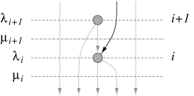
Figure 4: The probability that an edge (shown in bold) leaving vertex $i$ does not connect to vertex $i+1$ is given by $\lambda_{i+1}/\mu_{i+1}$.

Consider Fig. 4 and consider one of the ingoing edges at vertex $i$. That edge forms part of the flux $\mu_{i+1}$ immediately above $i$ and of that flux $k^{\mathrm{out}}_{i+1}$ edges, chosen uniformly at random, originate at vertex $i+1$, while the remaining $\mu_{i+1}-k^{\mathrm{out}}_{i+1}=\lambda_{i+1}$ flow around $i+1$, forming the excess flux at $i+1$. The probability that our particular edge is one of the ones flowing around $i+1$, i.e., that it does not originate at vertex $i+1$, is thus simply $\lambda_{i+1}/\mu_{i+1}$.

If our edge is to originate at vertex $j$, it must flow in this way around every intervening vertex from $i+1$ all the way up to $j-1$, and then finally it must originate at vertex $j$, which it does with probability $k^{\mathrm{out}}_{j}/\mu_{j}$. Multiplying the probabilities together, we find that the total probability of this particular edge originating at vertex $j$ is

$${k^{\mathrm{out}}_{j}\over\mu_{j}}\prod_{l=i+1}^{j-1}{\lambda_{l}\over\mu_{l}}=k^{\mathrm{out}}_{j}{\prod_{i+1}^{j-1}\lambda_{l}\over\prod_{i+1}^{j}\mu_{l}}.$$ (11)

This is just for one of the ingoing edges at vertex $i$. There are $k^{\mathrm{in}}_{i}$ such edges in all, so the total expected number of edges from $j$ to $i$ is

$$P_{ij}=k^{\mathrm{in}}_{i}k^{\mathrm{out}}_{j}{\prod_{i+1}^{j-1}\lambda_{l}\over\prod_{i+1}^{j}\mu_{l}}.$$ (12)

We will find it convenient to write this expression in the form

$$P_{ij}={k^{\mathrm{in}}_{i}k^{\mathrm{out}}_{j}\over m}f_{ij},$$ (13)

where

$$f_{ij}=m{\prod_{i+1}^{j-1}\lambda_{l}\over\prod_{i+1}^{j}\mu_{l}}.$$ (14)

The quantity $k^{\mathrm{in}}_{i}k^{\mathrm{out}}_{j}/m$ is the expected number of edges between $i$ and $j$ in an ordinary (not acyclic) directed random graph with the same degree sequence, so $f_{ij}$ represents the factor by which that expected number is modified in the acyclic graph. Alternatively, $f_{ij}$ is $m$ times the probability that a single in-stub at vertex $i$ is connected to a single out-stub at vertex $j$. (The probability itself vanishes in the limit of large graph size but with the inclusion of the factor of $m$ we get a quantity that tends to a nonzero limit, which will be useful when we come to consider properties of the graph as $n\to\infty$.)

One complication in the expression for $f_{ij}$ occurs if any flux in the denominator is zero. The expression gives the correct answer of zero for $P_{ij}$ if we adopt the convention that $0/0=1$. However, it’s usually better to analyze a graph divided by a zero flux cut as two independent graphs, since no edges cross the cut in such a network and the network forms two separate components. A network with zero excess flux does not necessarily form two separate components—the two parts of the network can by joined by a single common vertex at the top of one part and the bottom of the other—but the two parts can be treated independently anyway, with the shared vertex, if any, participating in both parts. Hence, in the following, we assume that $\mu_{i}\neq 0$ and $\lambda_{i}\neq 0$ except for $i=1$ and $i=n$.

Another useful expression for $f_{ij}$ can be derived by multiplying both sides of Eq. (14) by $f_{i^{\prime}j^{\prime}}$ with the condition that $i$ and $i^{\prime}$ are both less than $j$ and $j^{\prime}$. Then

$$f_{ij}f_{i^{\prime}j^{\prime}} ={\prod_{l=i+1}^{j-1}\lambda_{l}\over\prod_{l=i+1}^{j}\mu_{l}}\,{\prod_{l=i^{\prime}+1}^{j^{\prime}-1}\lambda_{l}\over\prod_{l=i^{\prime}+1}^{j^{\prime}}\mu_{l}}\ ={\prod_{l=i+1}^{j^{\prime}-1}\lambda_{l}\over\prod_{l=i+1}^{j^{\prime}}\mu_{l}}\,{\prod_{l=i^{\prime}+1}^{j-1}\lambda_{l}\over\prod_{l=i^{\prime}+1}^{j}\mu_{l}}$$

$$=f_{ij^{\prime}}f_{i^{\prime}j}.$$ (15)

Thus we can freely swap indices on a product of two overlapping $f$s. In particular, if we set $i^{\prime}=1$ and $j^{\prime}=n$, we find that

$$f_{ij}={f_{in}f_{1j}\over f_{1n}},$$ (16)

and $f_{ij}$ thus factors into a product of independent functions of $i$ and $j$. This result is of some practical use, since it implies that in order to calculate $f_{ij}$ or $P_{ij}$ for any $i$ and $j$ we need only the quantities $f_{in}$ and $f_{1j}$, which are $\mathrm{O}(n)$ in number and take $\mathrm{O}(n)$ time to calculate. Once these are known, we can calculate any $P_{ij}$ in $\mathrm{O}(1)$ time, which is as fast as the corresponding calculation for the configuration model, and far faster than direct application of Eq. (12), which takes $\mathrm{O}(n)$ time on average for each $P_{ij}$.

Perhaps the simplest way to implement this idea in practice is to define the two “dimensionless” quantities

$$a_{i}={f_{in}\over f_{1n}},\qquad b_{j}={f_{1j}\over f_{1n}},$$ (17)

so that

$$f_{ij}=f_{1n}a_{i}b_{j}.$$ (18)

Clearly $a_{1}=b_{n}=1$ and, substituting from Eq. (14) into Eq. (17), we find the values for other $i,j$ to be

$$a_{i} ={\prod_{l=2}^{i}\mu_{l}\over\prod_{l=2}^{i}\lambda_{l}}=\prod_{l=2}^{i}\biggl{(}1+{k^{\mathrm{out}}_{l}\over\lambda_{l}}\biggr{)},$$ (19a)

$$b_{j} ={\prod_{l=j+1}^{n}\mu_{l}\over\prod_{l=j}^{n-1}\lambda_{l}}=\prod_{l=j}^{n-1}\biggl{(}1+{k^{\mathrm{in}}_{l}\over\lambda_{l}}\biggr{)},$$ (19b)

where we have made use of Eq. (9) note2 . We will use these expressions in a number of calculations in the following sections.

III.5 Assortativity

As an example of the application of the calculations in the previous section, consider vertex correlations or “assortativity” in acyclic networks Newman (2003).

Consider a quantity $x$ defined on all vertices $i$ of a network. The network is said to be assortative with respect to $x$ if edges tend to connect vertices with similar values of $x$, high with high and low with low. Conversely, if edges connect dissimilar values, high with low and vice versa, then the network is said to be disassortative. Assortativity can be quantified by calculating a standard Pearson correlation coefficient $r$ over all pairs of values $x_{i},x_{j}$ on vertices $i,j$ connected by an edge. Positive values of $r$ indicate assortative networks, negative values disassortative ones.

In a directed network, such as the acyclic networks considered here, more complex types of correlations are also possible. For instance, one can consider two different quantities, $x$ and $y$, each defined on all vertices, and then ask about the correlations between pairs of values $x_{i},y_{j}$ on vertices $i,j$ connected by a directed edge from $j$ to $i$. (The simpler example above with only one quantity $x$ can be considered as the special case in which $y=x$.) Again one can calculate a correlation coefficient that quantifies the level of assortativity or disassortativity. The correlation coefficient is given explicitly in terms of the standard adjacency matrix by

$$r={1\over\sigma_{X}\sigma_{Y}}\,\biggl{[}{1\over m}\sum_{ij}A_{ij}x_{i}y_{j}-\mu_{\mathrm{in}}\mu_{\mathrm{out}}\biggr{]},$$ (20)

where

$$\mu_{\mathrm{in}}={1\over m}\sum_{i}k^{\mathrm{in}}_{i}x_{i},\qquad\mu_{\mathrm{out}}={1\over m}\sum_{j}k^{\mathrm{out}}_{j}x_{j},$$ (21)

and

$$\sigma_{X}^{2} ={1\over m}\sum_{i}k^{\mathrm{in}}_{i}x_{i}^{2}-\mu_{\mathrm{in}}^{2},$$ (22a)

$$\sigma_{Y}^{2} ={1\over m}\sum_{j}k^{\mathrm{out}}_{j}y_{j}^{2}-\mu_{\mathrm{out}}^{2}.$$ (22b)

Conventional random graph models such as the configuration model show no assortativity with respect to any quantity $x$, but random acyclic graphs can have nonzero assortativity. Consider Eq. (20) for the acyclic case and notice that the only dependence on $A_{ij}$ is in the first term of the numerator. All the other terms depend only on the degree sequence of the network, and hence are constant for our acyclic graph model over all members of the model ensemble. Averaging over the ensemble and noting that the model average of $A_{ij}$ is simply $P_{ij}$ from Eq. (13), we find that within our model

$$r ={1\over\sigma_{X}\sigma_{Y}}\,\biggl{[}{1\over m}\sum_{ij}P_{ij}x_{i}y_{j}-\mu_{\mathrm{in}}\mu_{\mathrm{out}}\biggr{]}$$

$$={1\over\sigma_{X}\sigma_{Y}}\,\biggl{[}{f_{1n}\over m^{2}}\sum_{i<j}a_{i}b_{j}k^{\mathrm{in}}_{i}k^{\mathrm{out}}_{j}x_{i}y_{j}-\mu_{\mathrm{in}}\mu_{\mathrm{out}}\biggr{]},$$ (23)

where we have used Eq. (18). In general, this expression can give nonzero values of $r$. We will see some examples in Section V for the particular case of assortativity with respect to vertex degree Pastor-Satorras et al. (2001); Newman (2002); Maslov et al. (2004), such as the case in which $x_{i}=k^{\mathrm{in}}_{i}$ and $y_{j}=k^{\mathrm{out}}_{j}$.

III.6 Large system-size limit

The developments so far are for a network of finite size with a specified degree sequence. Like other random graph models, however, random acyclic graphs become significantly simpler in a number of ways in the limit of large graph size. We examine that limit in this section.

Let the number of vertices in our network be $n$ as previously. In the limit of large $n$ we can no longer specify the complete degree sequence, since there are an infinite number of vertices, so, as with other random graphs, we specify instead a degree distribution, which is a joint probability distribution over in- and out-degrees as a function of vertex order. We define a “time” variable $t=i/n$ for the $i$th vertex, which falls in the range $0<t\leq 1$, then let $p_{t}(k^{\mathrm{in}},k^{\mathrm{out}})$ be the probability that a vertex at time $t$ has in- and out-degrees $k^{\mathrm{in}}$ and $k^{\mathrm{out}}$. Since vertices are uniformly distributed in time, this distribution is related to the overall (joint) degree distribution of the network by a simple integral:

$$p(k^{\mathrm{in}},k^{\mathrm{out}})=\int_{0}^{1}p_{t}(k^{\mathrm{in}},k^{\mathrm{out}})\>\mathrm{d}t.$$ (24)

Unfortunately the full distribution $p_{t}(k^{\mathrm{in}},k^{\mathrm{out}})$ is usually impossible to measure for an observed network: measuring it would require us to build a double histogram of $k^{\mathrm{in}}$ and $k^{\mathrm{out}}$ for many small intervals of $t$ and none of the real-world networks we have examined are large enough to give acceptable statistics for such a histogram. Luckily, however, it turns out that many interesting characteristics of the network can be calculated with a knowledge only of the moments of the degree distribution, and in most cases only the first moment, i.e., the mean degree.

The mean in- and out-degrees at time $t$ are given by

$$\bar{k}^{\mathrm{in}}(t) =\sum_{k^{\mathrm{in}}=0}^{\infty}\,\sum_{k^{\mathrm{out}}=0}^{\infty}k^{\mathrm{in}}p_{t}(k^{\mathrm{in}},k^{\mathrm{out}}),$$

$$\bar{k}^{\mathrm{out}}(t) =\sum_{k^{\mathrm{in}}=0}^{\infty}\,\sum_{k^{\mathrm{out}}=0}^{\infty}k^{\mathrm{out}}p_{t}(k^{\mathrm{in}},k^{\mathrm{out}}),$$ (25)

and the overall average degree $c$ of the network is

$$c=\int_{0}^{1}\bar{k}^{\mathrm{in}}(t)\>\mathrm{d}t=\int_{0}^{1}\bar{k}^{\mathrm{out}}(t)\>\mathrm{d}t.$$ (26)

Both $\bar{k}^{\mathrm{in}}(t)$ and $\bar{k}^{\mathrm{out}}(t)$ are easily measured in practice (at least approximately) by performing running averages of the observed degrees over suitably chosen time intervals.

For many of the calculations presented here we will use the rescaled quantities

$$\kappa^{\mathrm{in}}(t)={\bar{k}^{\mathrm{in}}(t)\over c},\qquad\kappa^{\mathrm{out}}(t)={\bar{k}^{\mathrm{out}}(t)\over c},$$ (27)

which satisfy the normalization conditions

$$\int_{0}^{1}\kappa^{\mathrm{in}}(t)\>\mathrm{d}t=\int_{0}^{1}\kappa^{\mathrm{out}}(t)\>\mathrm{d}t=1.$$ (28)

The quantity $\kappa^{\mathrm{in}}(t)\>\mathrm{d}t$ is the fraction of all in-stubs that are attached to vertices in the range $t$ to $t+\mathrm{d}t$, and similarly for $\kappa^{\mathrm{out}}(t)\>\mathrm{d}t$. The numbers of stubs are given by $m\kappa^{\mathrm{in}}(t)\>\mathrm{d}t$ and $m\kappa^{\mathrm{out}}(t)\>\mathrm{d}t$, since $m$ is the total number of stubs of each kind in the whole network.

The flux below vertex $i$ in the network is given by integrating these quantities up to a given vertex thus:

$$\mu_{i}=m\int_{0}^{t}\bigl{[}\kappa^{\mathrm{in}}(t^{\prime})-\kappa^{\mathrm{out}}(t^{\prime})\bigr{]}\mathrm{d}t^{\prime}.$$ (29)

where $t=i/n$ as before. Note that, assuming the degree distribution remains constant as the network becomes large, the integral for given $t$ also remains constant, but $m=nc$ grows with network size. Thus the flux becomes arbitrarily large as $n\to\infty$. For our purposes it is better to use a quantity that remains constant as $n$ varies and so we define a rescaled flux

$$\mu(t)={\mu_{i}\over m}=\int_{0}^{t}\bigl{[}\kappa^{\mathrm{in}}(t^{\prime})-\kappa^{\mathrm{out}}(t^{\prime})\bigr{]}\mathrm{d}t^{\prime}.$$ (30)

In the large system size limit, there is no difference between the flux $\mu$ and the excess flux $\lambda$: the two differ only by the number of stubs at a single vertex, which is a vanishing fraction of $m$ in the limit of large network size, and hence $\lambda_{i}$ also varies as $m$ and the rescaled excess flux $\lambda(t)=\lambda_{i}/m$ is given by

$$\lambda(t)=\int_{0}^{t}\bigl{[}\kappa^{\mathrm{in}}(t^{\prime})-\kappa^{\mathrm{out}}(t^{\prime})\bigr{]}\mathrm{d}t^{\prime}.$$ (31)

Physically $\mu(t)$ and $\lambda(t)$ are both equal to the fraction of edges that run from vertices after $t$ to vertices before.

Applying these definitions, we can now calculate a variety of quantities in the $n\to\infty$ limit. To calculate the probability of connection between two vertices, we start with Eq. (19a):

$$a_{i}=\prod_{l=2}^{i}\biggl{(}1+{k^{\mathrm{out}}_{l}\over\lambda_{l}}\biggr{)}=\exp\Biggl{[}\sum_{l=2}^{i}\ln\biggl{(}1+{k^{\mathrm{out}}_{l}\over\lambda_{l}}\biggr{)}\Biggr{]}.$$ (32)

Observing, as above, that $\lambda_{l}$ goes as $m$ in the large system size limit while $k^{\mathrm{out}}_{l}$ remains constant and keeping terms to leading order, this becomes

$$a_{i}=\exp\Biggl{[}\sum_{l=2}^{i}{k^{\mathrm{out}}_{l}\over\lambda_{l}}\Biggr{]}.$$ (33)

And in the limit of large $n$, the sum becomes an integral:

$$a(t)=\exp\biggl{[}\int_{0}^{t}{\kappa^{\mathrm{out}}(t^{\prime})\over\lambda(t^{\prime})}\>\mathrm{d}t^{\prime}\biggr{]}.$$ (34)

Similarly, defining $u=j/n$, Eq. (19b) becomes

$$b(u)=\exp\biggl{[}\int_{u}^{1}{\kappa^{\mathrm{in}}(u^{\prime})\over\lambda(u^{\prime})}\>\mathrm{d}u^{\prime}\biggr{]},$$ (35)

and substituting both into Eq. (18) we get

$$f(t,u)=f(0,1)\,a(t)\,b(u),$$ (36)

where $f_{ij}=f(i/n,j/n)$. Physically, $f(t,u)$ is $m$ times the probability that an in-stub at time $t$ is connected to an out-stub at time $u$. The normalizing constant $f(0,1)$ can be calculated by noting that every in-stub must be connected to some out-stub, which means that

$$\int_{t}^{1}f(t,u)\,\kappa^{\mathrm{out}}(u)\>\mathrm{d}u=1.$$ (37)

Substituting for $f(t,u)$ from Eq. (36) and setting $t=0$ then gives

$$f(0,1)=\biggl{[}\int_{0}^{1}b(u)\kappa^{\mathrm{out}}(u)\>\mathrm{d}u\biggr{]}^{-1},$$ (38)

where we have made use of $a(0)=1$. If we instead normalize by integrating over $t$ we get the alternative form

$$f(0,1)=\biggl{[}\int_{0}^{1}a(t)\kappa^{\mathrm{in}}(t)\>\mathrm{d}t\biggr{]}^{-1},$$ (39)

which gives the same answer but may be more convenient in some cases, depending on the forms of $\kappa^{\mathrm{in}}$ and $\kappa^{\mathrm{out}}$.

Armed with a value for $f(t,u)$ we can now calculate the expected number of edges between two vertices in the network from Eq. (13):

$$P_{ij}={k^{\mathrm{in}}_{i}k^{\mathrm{out}}_{j}\over m}f(i/n,j/n).$$ (40)

Alternatively, we can average this expression over the distributions of $k^{\mathrm{in}}$ and $k^{\mathrm{out}}$ to get the average number of edges between a vertex at $t$ and another at $u$:

$$P(t,u)={\bar{k}^{\mathrm{in}}(t)\bar{k}^{\mathrm{out}}(u)\over m}f(t,u)={c\over n}\kappa^{\mathrm{in}}(t)\kappa^{\mathrm{out}}(u)f(t,u).$$ (41)

Since $f(t,u)$ is independent of $n$ for given $\kappa^{\mathrm{in}}(t)$ and $\kappa^{\mathrm{out}}(u)$, $P_{ij}$ [and $P(t,u)$] goes as $1/n$ in a sparse graph as graph size becomes large and hence vanishes in the limit. This allows us to interpret $P_{ij}$ as a probability of connection between vertices in the $n\to\infty$ limit—the expected number of edges and the probability of connection are the same when both become small.

We also note in passing the following useful relation between $\lambda(t)$ and $f(t,u)$. From Eq. (12) we have

$$P_{i-1,i}={k^{\mathrm{in}}_{i-1}k^{\mathrm{out}}_{i}\over\mu_{i}},$$ (42)

so that $f_{i-1,i}=m/\mu_{i}$. Setting $t=i/n$ as before and $\mu_{i}/m=\lambda(t)$, this implies that

$$\lambda(t)={1\over f(t,t)}.$$ (43)

III.7 Examples

To illustrate the application of these results let us look at some concrete examples. Consider a network with average degrees $\bar{k}^{\mathrm{in}}(t)=2c(1-t)$ and $\bar{k}^{\mathrm{out}}(t)=2ct$, where $c$ is now a free parameter controlling the overall mean degree. Then

$$\kappa^{\mathrm{in}}(t)=2(1-t),\qquad\kappa^{\mathrm{out}}(u)=2u,$$ (44)

and we find that

$$f(t,u)=\frac{1}{2(1-t)u}$$ (45)

and

$$P(t,u)=\frac{2c(1-t)\times 2cu}{2m(1-t)u}=\frac{2c}{n},$$ (46)

where we have used $m=nc$ in the second equality.

Thus the expected number of edges between every pair of vertices in this case is the same, and indeed one could exploit this fact to create a network with the degree sequence above by taking an initially empty graph and placing a directed edge between each vertex pair with uniform probability $2c/n$, oriented to point from the “later” vertex to the “earlier” one. Such a model has been studied previously as a model of food webs, in which context it is known as the cascade model Cohen and Newman (1985). It’s easy to see that the cascade model produces networks with a given degree sequence uniformly at random and thus is approximately equivalent to an acyclic random graph with the same degree sequence as described in this paper. The equivalence is only approximate: the cascade model has a Bernoulli distribution of edges between any two vertices while our model has a Poisson distribution. This difference, however, vanishes in the limit of large graph size, where the edge probability becomes small, and thus in this limit the two models are the same.

More generally, consider a model where a Poisson distributed number of directed edges is placed between all pairs of vertices $i,j$ with $i<j$. If the mean of the Poisson distribution for each vertex pair can be written as a product of a quantity $r_{i}$ that depends on $i$ but not on $j$ and a quantity $s_{j}$ that depends on $j$ but not on $i$, then the model produces acyclic random graphs conditioned on the degree sequence. To prove this we write the probability $P$ of generating a particular graph thus:

$$P=\prod_{i<j}\mathrm{e}^{-s_{i}r_{j}}\frac{(s_{i}r_{j})^{A_{ij}}}{A_{ij}!}=\frac{\prod_{i<j}\mathrm{e}^{-s_{i}r_{j}}}{\prod_{i<j}A_{ij}!}\prod_{i}s_{i}^{k^{\mathrm{in}}_{i}}r_{i}^{k^{\mathrm{out}}_{i}}.$$ (47)

The factor $\prod_{i<j}\mathrm{e}^{-s_{i}r_{j}}$ is a constant for all graphs and the factor $\prod_{i}s_{i}^{k^{\mathrm{in}}_{i}}r_{i}^{k^{\mathrm{out}}_{i}}$ is constant for a given degree sequence. Thus the only variation in the probability $P$ for graphs of given degree sequence comes from the factor $\prod_{i<j}A_{ij}!$. But this is the same factor by which the probability of such graphs varies in the random acyclic graph model—see Section III.2—and thus, for a given degree sequence, the model above produces graphs with the same probabilities as the random acyclic graph and the two models have identical ensembles. The cascade model is a particularly simple instance of this situation in which $r_{i}$ and $s_{j}$ are both constant.

As another example, we consider networks with power-law degree distributions, which have received a lot of attention in the recent networks literature. In particular, for reasons that will shortly become clear, we consider networks generated by linear preferential attachment processes Barabási and Albert (1999), which naturally generate directed acyclic graphs and have long been used as models of citation networks Price (1976). We consider the general model in which vertices added continually to a growing network make $c$ directed connections each to previously existing vertices chosen at random in proportion to the current in-degrees of those vertices plus a constant $r$. This process produces networks with overall in-degree distributions having a power-law tail $p(k)\sim k^{-\alpha}$ where $\alpha=2+r/c$ Price (1976); Dorogovtsev et al. (2000). In the notation used in this paper the average in-degree as a function of time is given by Dorogovtsev et al. (2000):

$$\kappa^{\mathrm{in}}(t)=(\alpha-2)(t^{-1/(\alpha-1)}-1),$$ (48)

and $\kappa^{\mathrm{out}}(u)=1$.

Let us consider a random directed acyclic graph built on degree sequences generated by the linear preferential attachment model and let us calculate the probability of connection between vertices. Feeding the expressions above for $\kappa^{\mathrm{in}}(t)$ and $\kappa^{\mathrm{out}}(u)$ into our earlier formulas, we find that

$$f(t,u)=\frac{1}{(\alpha-1)(1-t^{1/(\alpha-1)})u^{(\alpha-2)/(\alpha-1)}}$$ (49)

and

$$P(t,u)=c(\alpha-2)i^{-1/(\alpha-1)}j^{-(\alpha-2)/(\alpha-1)},$$ (50)

where again $t=i/n$ and $u=j/n$. Remarkably, this is precisely the average probability of an edge between vertices in the preferential attachment model itself Dorogovtsev and Mendes (2002). Indeed, as we will shortly show, the linear preferential attachment ensemble and the ensemble of the random acyclic graph with the same degree sequence are actually identical, because linear preferential attachment, conditioned on the degree sequence, produces matchings uniformly at random, which is precisely the condition for the random acyclic graph. Thus, not only is $P(t,u)$ the same for the two models, but all properties of the models are identical and one can properly say that the linear preferential attachment model is a special case of the random directed acyclic graph.

This is an important point. It is often claimed that networks produced by the linear preferential attachment process are, in some sense, not really random, being nonuniform in their ensemble properties because they are grown according to a nonequilibrium growth process. In fact, however, this is not the case. Once the acyclic nature of the networks is taken into account, the ensemble of the linear preferential attachment model is perfectly uniform for a given degree sequence.

To prove this we compute the probability of a particular matching being produced by the linear preferential attachment model as a function of in-degree sequence. An outgoing edge at a newly added vertex $j$ in the growing preferential attachment network attaches to a previous vertex $i$ with probability proportional to $i$’s current in-degree $k^{\mathrm{in}}_{i}$ plus the constant $r$. The correctly normalized probability of attachment is

$${k^{\mathrm{in}}_{i}+r\over\sum_{i=1}^{j-1}(k^{\mathrm{in}}_{i}+r)}={k^{\mathrm{in}}_{i}+r\over m+(j-1)r},$$ (51)

where $m=\sum_{i}k^{\mathrm{in}}_{i}$ is the current number of edges in the network. The probability of the entire matching is given by the product of this expression over all edges. Let us consider the numerator and denominator of the product separately, starting with the numerator.

The current in-degree of vertex $i$ is 0 when the first edge attaches to it, 1 when the second edge attaches, and so forth. Hence the factors for vertex $i$ in the numerator are

$$r(1+r)\ldots(k^{\mathrm{in}}_{i}-1+r)={\Gamma(k^{\mathrm{in}}_{i}+r)\over\Gamma(r)},$$ (52)

where $k^{\mathrm{in}}_{i}$ now represents the final in-degree of $i$ at the end of the growth process and $\Gamma(x)$ is the standard gamma function. Taking the product over all vertices, the complete numerator is $\prod_{i=1}^{n-1}\Gamma(k^{\mathrm{in}}_{i}+r)/\Gamma(r)$. (There is no term for the last vertex since it necessarily has no ingoing edges.)

For the denominator, we note that the number of edges $m$ in the network increases by one for each edge added and takes the value $(j-2)c$ for the first edge added with vertex $j$ and $(j-1)c-1$ for the last. Thus the factors in the denominator corresponding to the edges added with vertex $j$ give

$$[(j-2)c+(j-1)r]\ldots[(j-1)c-1+(j-1)r]$$

$$\hskip 100.00015pt{}={\Gamma((j-1)(c+r))\over\Gamma((j-1)(c+r)-c)},$$ (53)

and the complete denominator is

$$\prod_{j=2}^{n}{\Gamma((j-1)(c+r))\over\Gamma((j-1)(c+r)-c)}=\prod_{i=1}^{n-1}{\Gamma(i(c+r))\over\Gamma(i(c+r)-c)}.$$ (54)

Dividing numerator by denominator, the complete probability for the matching is then

$$P=\prod_{i=1}^{n-1}{\Gamma(k^{\mathrm{in}}_{i}+r)\over\Gamma(r)}\,{\Gamma(i(c+r)-c)\over\Gamma(i(c+r))}.$$ (55)

Since this probability depends only on the degree sequence and not on any details of which vertices attach to which others, it follows that the preferential attachment process generates all matchings with a given degree sequence with the same probability, and hence that the set of networks with that degree sequence constitutes a random directed acyclic graph of the type considered in this paper.

Note that a calculation similar to the one above can be performed for a model in which out-degree is not the same for every vertex, but varies from one vertex to another, or a network in which the parameter $r$ varies between vertices. The probability of a particular matching for such a model is still a function only of the degrees and other parameters and not of the pattern of connections in the network and hence the network is still a random graph of the type considered here.

IV Random directed acyclic graphs with independent edge probabilities

In this section we define the second of our two random graph models for acyclic graphs. In this model rather than fixing the degree of each vertex we fix only the expected degree. As discussed in the introduction the model is in some ways analogous to the $G(n,p)$ model of Erdős and Rényi Erdős and Rényi (1959) for ordinary (Poisson) random graphs, while the previous model is the equivalent of $G(n,m)$.

We have seen that it is possible in our previous model to calculate the probability of an edge between any pair of vertices. However, in that model edges are not independent because the presence of one edge connecting to a given vertex $i$ reduces the number of stubs available for other edges and hence reduces the probability of edges from other vertices. In the limit of large network size, the probabilities for edges to and from intervals $\mathrm{d}t$ and $\mathrm{d}u$ become independent, but even in this limit edges that share the same exact vertex, either as source or target, remain correlated.

The same phenomenon is also seen in other random graph models, such as the configuration model, in which degrees are also fixed and the presence of one edge to a vertex reduces the probability of others. In that case, researchers have found it useful to study a slightly different model in which edges are placed with the same probability as in the configuration model, but independently Chung and Lu (2002a, b); Bollobás et al. (2007). The same strategy turns out also to work well in the case of acyclic graphs. The resulting model is described in this section.

IV.1 Definition of the model

Our second model is defined as follows: starting with an empty graph of $n$ vertices we generate for each pair of vertices $i,j$, with $i<j$, a Poisson distributed number with mean $P_{ij}$ and place that number of edges between $i$ and $j$, pointing from $j$ to $i$. The values of $P_{ij}$ are typically calculated from a desired degree sequence using Eq. (13), and the resulting network trivially has the same expected number of edges between every vertex pair as the network generated by our first model with the same degree sequence, but the edges are now, by construction, independent.

Since the number of edges between every vertex pair is Poisson distributed, so also is the total number of edges $m$. Thus an equivalent way to create networks drawn from this model is to generate a Poisson distributed random number $m$ with mean equal to the desired expected number of edges, then distribute those edges at random over the graph in proportion to $P_{ij}$. This second method for generating networks is a more efficient one for numerical work but the first is more convenient for analytic treatment of the model.

The principal disadvantage of this model is that it does not allow us to fix the exact degrees of each vertex. Instead we can only fix the expected degrees $\bar{k}^{\mathrm{in}}_{i}$ and $\bar{k}^{\mathrm{out}}_{i}$. The expected in-degree, for instance, is given by $\sum_{j=i+1}^{n}P_{ij}$, which is by definition equal to the value of $k^{\mathrm{in}}_{i}$ used to calculate $P_{ij}$ in the first place. In other words, the network has expected degrees equal to the chosen degree sequence, but the actual degrees may be different.

In fact, since the numbers of edges are Poisson independent variables, the in-degree will also be Poisson distributed with mean $k^{\mathrm{in}}_{i}$ (and similarly for the out-degree). Note however that this does not mean that the overall distribution of the degrees at any time has to be Poisson, since the distribution from which the means themselves are drawn can be anything we like and the overall distribution of degrees is a convolution of this distribution and the Poisson distribution.

The expected degrees also need not be integers, so this model allows a slight generalization of the previous one in that the values of $k^{\mathrm{in}}_{i}$ and $k^{\mathrm{out}}_{i}$ we use to calculate $P_{ij}$ need not be integers. Indeed we could generalize the model considerably further, since in principle we can choose the values of the $P_{ij}$ to be anything we want, including values that cannot be generated from Eq. (13) by any choice of degrees. Any values, for example, that do not take the product form of Eq. (13) fall in this category. In this paper, however, we will mostly be concerned with choices of $P_{ij}$ that correspond to an underlying choice of expected degrees.

IV.2 Computer generation of networks

It is less straightforward to numerically generate networks drawn from the ensemble of our second model than of our first. The basic approach is as outlined above: given the expected degrees, we calculate the expected number of edges by summing $\overline{m}=\sum_{i=1}^{n}k^{\mathrm{in}}_{i}$ and then generate a Poisson distributed number with this mean, which will be the actual number of edges $m$.

To place these $m$ edges with the appropriate probabilities we need to be able to randomly generate vertex pairs with probabilities proportional to $P_{ij}$. This can conveniently be achieved by making use of the product form (13) of $P_{ij}$. We draw a value for $i$ from the marginal probability distribution, which goes as $\sum_{j=i+1}^{n}P_{ij}=k^{\mathrm{in}}_{i}$, using a standard transformation method, which takes $\mathrm{O}(\log n)$ time. Then we draw a value for $j$ between $i+1$ and $n$ in proportion to $k^{\mathrm{out}}_{j}b_{j}$, again using the transformation method. Then we place an edge between $i$ and $j$ and repeat for the next edge. When all $m$ edges have been placed the graph is complete. The whole process takes $\mathrm{O}(n)$ time for set-up and $\mathrm{O}(m\log n)$ for selection and placing of edges, or $\mathrm{O}(n+m\log n)$ time in total, which is $\mathrm{O}(n\log n)$ on a graph with fixed degree distribution so that $m\propto n$.

V Comparison with empirical data

Our expressions for edge probabilities allow us to make a comparison between our model networks and their counterparts in the real world. We focus on citation networks, which are the largest and best documented examples of acyclic networks.

The simplest comparison we could make would be a direct comparison of edge probabilities $P_{ij}$. However, the value of $P_{ij}$ is strongly influenced by the degrees of vertices—the initial factor of $k^{\mathrm{in}}_{i}k^{\mathrm{out}}_{j}$ in Eq. (13)—which makes comparison plots noisy and difficult to interpret by eye. A cleaner comparison is of the stub probability $f_{ij}$, Eq. (14), which is $m$ times the probability that a stub at vertex $i$ is connected to a stub at vertex $j$.

We can make an estimate of $f_{ij}$ for an observed network by taking a window of vertices around $i$ and another around $j$, counting the number of edges between vertices in the two windows, and then dividing in turn by the number of in-stubs in the first window and out-stubs in the second and multiplying by $m$ note3 . If the windows are large enough to provide good statistics but small enough to span only a relatively narrow range of $i$ and $j$ then one can get good estimates of the mean stub probability this way.

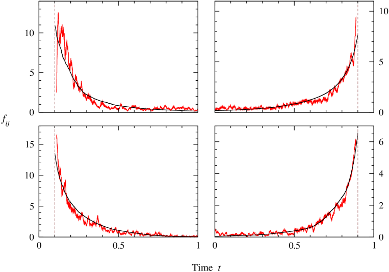
Figure 5: Comparison of empirical measurements (red) and analytic predictions (black) of $f_{ij}$ for the two citation networks described in the text: preprints on high-energy physics (top) and cases of the United States Supreme Court (bottom). The left panel in each case shows $f_{ij}$ for citations from times $t$ to time $0.1$ (indicated by dashed line). The right panel shows $f_{ij}$ for citations to times $t$ from time $0.9$. Empirical measurements were averaged over windows of size $300$ vertices.

In Fig. 5 we show the results of such measurements for two citation networks. The first is a network of citations between academic papers in the area of theoretical high-energy physics, which we studied previously in Ref. Karrer and Newman (2009). This data set comprises $27\,221$ papers posted in the “hep-th” section of the Physics E-print Archive at arxiv.org between January 1992 and February 2003. The data set was compiled by the organizers of the KDD Cup challenge, a data analysis competition run as part of the annual ACM SIGKDD conference, and incorporates citations extracted from data held in the SPIRES database at the Stanford Linear Accelerator Center.

The second data set is a network of citations between $26\,084$ legal decisions handed down by the United States Supreme Court, from the time of the court’s inception in 1789 until 2006, as compiled by Leicht et al. Leicht et al. (2007).

From these data we extracted values for $f_{ij}$ as described and also calculated the full in- and out-degree sequences and used them to evaluate the analytic expression (14) for the same quantity.

Figure 5 shows separately the value of $f_{ij}$ for fixed $i$ and varying $j$ (left panels) and for fixed $j$ and varying $i$ (right panels) for the two networks. As we can see, in all cases the analytic solution for the random graph model agrees surprisingly well with the measurements. The agreement is not perfect—there are visible differences between measurement and theory—but the level of agreement is far better than for most other random graph models. Certainly the predictions of the configuration model rarely agree this well with the behavior of real-world networks. Thus it appears that, in this case at least, the twin inputs of degree sequence and vertex order are enough to capture a large part of the variation in edge placement in the true citation networks.

There are other aspects of network structure, however, that are not so well captured by our model. An example is correlations between the degrees of adjacent vertices, or degree assortativity in the nomenclature of Section III.5. We consider two kinds of possible degree correlations over directed edges: correlations between in- and out-degrees at the start and end of directed edges, and correlations between in-degrees at either end. In the language of paper citations, the former is a measure of the extent to which highly cited papers are cited more often by prolific citers. The latter is a measure of the extent to which highly cited papers are more likely to be cited by other highly cited papers. We have computed correlation coefficients of the form (20) for both networks described above for both of these types of correlations, as well as calculating expected values for random graphs with the same degree sequences from Eq. (20).

The results show mixed levels of agreement. For the high-energy physics citation network the measured and predicted values of the correlation coefficients are in all cases very small, indeed negligible for most practical purposes, so that, although the empirical and theoretical values do not agree closely, one could claim that there is qualitative agreement between them in that there is essentially no correlation present. [For in-degree/out-degree correlations we find $r=0.002$ (empirical) and $-0.003$ (theory) and for in-degree/in-degree we find $r=0.040$ (empirical) and $0.016$ (theory).]

For the Supreme Court, on the other hand, the correlations are more substantial and moreover display significant disparity between observed and predicted values. For in-degree/out-degree correlations we find $r=0.124$ (empirical) and $0.007$ (theory), and for in-degree/in-degree we find $r=0.184$ (empirical) and $0.022$ (theory). This appears to indicate the presence of significant phenomena in the real network that are not captured in the model, and illustrates one of the main motivations for the creation of random graph models, which is to provide a null model that can tell us when an observed property of a network differs significantly from what we would expect on the basis of chance, and hence draw our attention to nontrivial network features.

VI Conclusions

In this paper we have introduced two random graph models for directed acyclic graphs, which are analogous to the $G(n,m)$ and $G(n,p)$ models of traditional random graph theory. We have defined and calculated a number of fundamental theoretical quantities for these models, including degree sequences, degree distributions, edge and stub probabilities, and degree correlations. We have also defined the appropriate infinite-size limit of our models and shown that a number of the central quantities of the theory simplify in this limit. We have compared the basic predictions of the models with two example real-world networks, a network of citations between physics papers and another of legal decisions, finding surprisingly good agreement between measurement and theory for some properties, but significant divergence in others.

Starting with the formalism developed in this paper it should be possible to compute many other standard network quantities for random directed acyclic graphs. We believe that the models developed here have the potential to shed a significant amount of light on the effects of vertex ordering, an important defining property in many real-world networks.