Learning Object Location Predictors with Boosting and Grammar-Guided Feature Extraction

Abstract

We present Beamer: a new spatially exploitative approach to learning object detectors which shows excellent results when applied to the task of detecting objects in greyscale aerial imagery in the presence of ambiguous and noisy data. There are four main contributions used to produce these results. First, we introduce a grammar-guided feature extraction system, enabling the exploration of a richer feature space while constraining the features to a useful subset. This is specified with a rule-based generative grammar crafted by a human expert. Second, we learn a classifier on this data using a newly proposed variant of AdaBoost which takes into account the spatially correlated nature of the data. Third, we perform another round of training to optimize the method of converting the pixel classifications generated by boosting into a high quality set of $(x,y)$ locations. Lastly, we carefully define three common problems in object detection and define two evaluation criteria that are tightly matched to these problems. Major strengths of this approach are: (1) a way of randomly searching a broad feature space, (2) its performance when evaluated on well-matched evaluation criteria, and (3) its use of the location prediction domain to learn object detectors as well as to generate detections that perform well on several tasks: object counting, tracking, and target detection. We demonstrate the efficacy of Beamer with a comprehensive experimental evaluation on a challenging data set.

1 Introduction

Learning to detect objects is a subfield of computer vision that is broad and useful with many applications. This paper is concerned with the task of unstructured object detection: the input to the object detector is an image with an unknown number of objects present, and the output is the locations of the objects found in the form of $(x,y)$ pairs, and perhaps delineating them as well. A typical application is detection of cars in aerial imagery for purposes such as car counting for traffic analysis, tracking, or target detection. Figure 1 shows (a) an example image from the data set used in the experiments, (b) its mark-up, (c) an example of an initial confidence-rated weak hypothesis learned on it, and subfigures (d-i) show some of the trickier examples in the data set.

Section 2 reviews common approaches to object detection. Section 3.2 describes a new variant of AdaBoost that takes into account the spatially correlated nature of the data to reduce the effects of label noise, simplify solutions, and achieve good accuracy with fewer features. Section 3.1 describes our technique for generating features randomly but guided by a stochastic grammar crafted by a domain expert to make useful features more likely, and unhelpful features, less likely. A second round of training involves learning detectors which predict $(x,y)$ locations of objects from pixel classifications, described in Section 3.3. Since the quality of detections greatly depends on the problem at hand, two different evaluation criteria are carefully formulated to closely match three common problems: tracking, target detection, and object counting. Lastly, in our evaluation Section 4, each component in the detection pipeline is isolated and compared against alternatives through an extensive validation step involving a grid search over many parameters on the two different metrics. The results are used to gain insights into what leads to a good object detector. We have found our contributions give better results.

2 Background

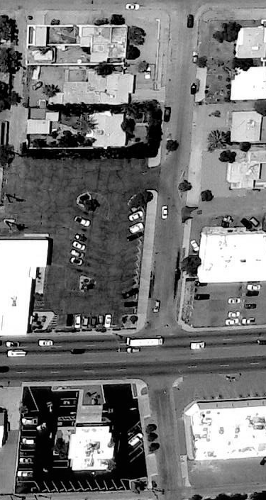
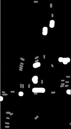
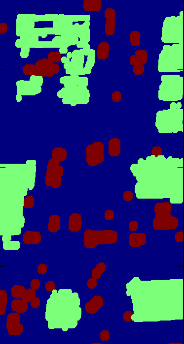
			(d) (e) (f)
(a)	(b)	(c)	(g)	(h)	(i)

Figure 1: An aerial photo of Phoenix, AZ was divided into 11 slices. An example slice is shown in subfigure (a). Its mark-up is shown in subfigure (b); background pixels are black, object pixels are grey, and confuser pixels, white. Subfigure (c) shows an example of a post processing applied to a weak hypothesis, which helps disambiguate between similar car and building patches by abstaining on building pixels. Cars are indicated by red, background by blue and abstention by green. Examples of ambiguous objects include (d) a roof-mounted air-conditioner, (e) an overhead street sign, (f) vegetation, (g) closely packed cars, (h) a dark car, and (i) a car on a roof carpark in partial shadow.

Localizing objects in an image is a prevalent problem in computer vision known as object detection. Object recognition, on the other hand, aims to identify the presence or absence of an object in an image. Many object detection approaches reduce object detection to object recognition by employing a sliding window [Viola and Jones(2001), Ferrari et al.(2008)Ferrari, Fevrier, Jurie, and Schmid, Laptev(2006)], one of the more common design patterns of an object detector. A fixed sized rectangular or circular window is slid across an image, and a classifier is applied to each window. The classifier usually generates a real-valued output representing confidence of detection. Often this method must carefully arbitrate between nearby detections to achieve adequate performance.

Object detection models can be loosely be broken down into several different overlapping categories. Parts-based based models consider the presence of parts and (usually) the positioning of parts in relation to one another [Fergus et al.(2003)Fergus, Perona, and Zisserman, Agarwal et al.(2004)Agarwal, Awan, and Roth, Chum and Zisserman(2007)]. A special case is the bag of words model where predictions are made simply on the presence or absence of parts rather than their overall structure or relative positions [Heisele et al.(2003)Heisele, Ho, Wu, and Poggio, Zhang et al.(2007)Zhang, Marszalek, Lazebnik, and Schmid]. Some parts-based models model objects by their characterizing shape during learning and matching shape to detect [Belongie et al.(2002)Belongie, Malik, and Puzicha]. Cascades are commonly used to reduce false positives and improve computational efficiency. Rather than applying a single computationally expensive classifier to each window, a sequence of cheaper classifiers is used. Later classifiers are invoked only if the previous classifiers generate detections. Generative model approaches learn a distribution on object appearances or object configurations [Mikolajczyk et al.(2006)Mikolajczyk, Leibe, and Schiele]. Segmentation-based approaches fully delineate objects of interest with polygons or pixel classification [Shotton et al.(2008)Shotton, Johnson, and Cipolla]. Contour-based approaches identify contours in an image before generating detections [Ferrari et al.(2008)Ferrari, Fevrier, Jurie, and Schmid, Opelt et al.(2006)Opelt, Pinz, and Zisserman]. Descriptor vector approaches generate a set of features on local image patches. One of the most commonly used descriptors is the Scale Invariant Feature Transform (SIFT), which is invariant to rotation, scaling, and translation and robust to illumination and affine transformations [Lowe(1999)]. A large number of object detectors use interest point detectors to find salient, repeatable, and discriminative points in the image as a first step [Dorkó and Schmid(2003), Agarwal et al.(2004)Agarwal, Awan, and Roth]. Feature descriptor vectors are often computed from these interest points. Probabilistic models estimate the probability of an object of interest occurring; generative models are often used [Schneiderman and Kanade(2000), Fergus et al.(2003)Fergus, Perona, and Zisserman]. Feature Extraction creates higher level representations of the image that are often easier for algorithms to learn from. Heisele, et al [Heisele et al.(2003)Heisele, Ho, Wu, and Poggio] train a two-level hierarchy of support vector machines: the first level of SVMs finds the presence of parts, and these outputs are fed into a master SVM to determine the presence of an object. Dorko, et al [Dorkó and Schmid(2003)] use an interest point detector, generate a SIFT description vector on the interest points, and then use an SVM to predict the presence or absence of objects.

One of the more popular and highly regarded feature-based object detectors is the sliding window detector proposed by Viola and Jones [Viola and Jones(2001)], which uses a feature set originally proposed by Papageorgiou, et al [Papageorgiou et al.(1998)Papageorgiou, Oren, and Poggio]. Adjacent rectangles of equal size are filled with $1$s and $-1$s and embedded in a kernel filled with zeros. The kernel is convolved with the image to produce the feature and using an integral image greatly reduces the computation time for these features. Viola and Jones employ a cascaded sliding window approach where each component classifier of the cascade is a linear combination of weak classifiers trained with AdaBoost.

3 Approach

The Beamer object detector pipeline consists of a feature extraction stage, pixel classification stage, and a detector stage as Figure 2 shows. First, a set of learned features are combined into a pixel classifier using AdaBoost [Freund and Schapire(1996)]. Then, the detector pipeline (see Section 3.3) transforms the pixel classifications into a set of $(x,y)$ locations representing the predicted locations of the objects. Our methodology partitions the data set into training, validation, and test image sets. The pixel classifier is learned during the training phase on the training images with the grammar constraints, post-processing parameters, and stopping conditions remaining fixed. These fixed parameters are later tuned on the validation set along with the detector’s parameters. The detector generates $(x,y)$ location predictions from the pixel classification. After the training and validation steps, a fully learned object detector results. The grey arrows show how data flows through a specific instance of an object detector.

Section 3.1 describes the very first step of weak pixel classification, feature extraction, which is carried out by generating features with a generative grammar. Section 3.2 describes the learning of an ensemble of weak pixel classifications using boosting. Finally, Section 3.3 explains how the pixel classification ensemble is transformed into $(x,y)$ location domain predictions. A complete list of all the parameters described in the following sections is given in Table 2.

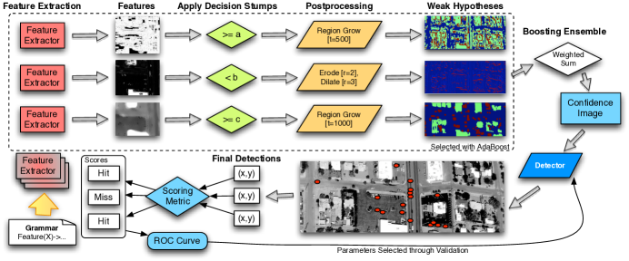
Figure 2: Object detection is carried out in a pipeline consisting of three stages: feature extraction, pixel classification, and locality predictions in the form of $(x,y)$. At each training iteration, a new pool of feature extractors generated by a grammar. Beamer then chooses the best feature extractor, decision stump, and post-processing filter combination. Thresholding these features yields a weak pixel classification which are combined with AdaBoost to produce a confidence image. The grey arrows show the flow of data to carry out object detection from start to finish for a static instance of an object detector.

3.1 Feature Extraction

A single pixel in a greyscale image provides very limited information about its class. Feature extraction is helpful for generating a more informative feature vector for each pixel, ideally incorporating spatial, shape, and textural information. This paper considers extracting features with neighborhood image operators such as convolution and morphology. Even good sets of neighborhood-based features are unlikely to have enough information to perfectly predict labels, but the hope is that large and diverse sets of features can encode enough information to make adequate predictions. At each boosting iteration, a new set of random features is generated, but only the best feature of this set is kept.

Generative grammars are common structures used in Computer Science to specify rules to define a set of strings [Sipser(2005), Hopcroft and Ullman(1990)]. Extending our earlier work on time series [Eads et al.(2005)Eads, Glocer, Perkins, and Theiler], we use them to specify the space of feature extraction programs, which are represented as directed graphs (a graph representation is preferable because it allows for re-use of sub-computations). A grammar is made up of nonterminal productions such as $P\rightarrow A|B$, which are expanded to generate a new string. The rules associated with the production are selected at random, so $P$ can be expanded as either $A$ or $B$. Figure 3 shows an example graph program generated by the Beamer grammar shown in Figure 4. The primitive operators used for our object detection system are listed in Table 1 and the grammar governing how they are combined is shown in Figure 4.

Figure 3: An example of a feature extractor program generated by the Beamer grammar which is achieved by reducing $\mathtt{Feature}(I)$ using the production rules of the grammar (where $I$ is an image variable), $\mathtt{Feature}(I)\rightarrow\mathtt{Compound}(I)\rightarrow\mathtt{Binary}(I,\mathtt{Compound}(I))\rightarrow\mathtt{Binary}(I,\mathtt{Unary}(I))\rightarrow\mathtt{Binary}(I,\mathtt{NLUnary}(I))\rightarrow\mathtt{Binary}(I,\mathtt{Morph}(I,\mathtt{RandomSE}))\rightarrow\mathtt{Binary}(I,\mbox{erode}(I,\mathtt{RandomSE}))\rightarrow\mathtt{Binary}(I,\mbox{erode}(I,(^{\prime}ellipse^{\prime},pi/2,8,0.3)))\rightarrow\mbox{normDiff}(I,\mbox{erode}(I,(^{\prime}ellipse^{\prime},pi/2,8,0.3)))$

Function	Description
mult($I_{A}$, $I_{B}$)	Element-wise multiplies two images, $f(a,b)=ab$.
blend($I_{A}$, $I_{B}$)	Element-wise averaging of two images, $f(a,b)=\frac{a+b}{2}$.
normDiff($I_{A}$, $I_{B}$)	Normalized difference, $f(a,b)=\frac{a-b}{\sum_{p\in I_{A}}{p}+\sum_{p\in I_{B}}{p}}$.
scaledSub($I_{A}$, $I_{B}$)	Scaled difference, $f(a,b)=\frac{a-b}{a+b}$.
sigmoid($I$, $\theta$, $\lambda$)	Soft maximum with threshold $\theta$ and scale $\lambda$, $f(u)=\frac{\arctan(\lambda(u+\theta))}{\lambda}$
ggm(I, $\sigma$)	Applies a Gaussian Gradient Magnitude to an image.
laplace(I, $\sigma$)	Laplace operator with Gaussian 2nd derivatives & standard deviation $\sigma$.
laws(I, $u$, $v$)	Applies the Laws texture energy kernel $u\cdot v$.
gabor(I, $\theta$, $k$, $r$, $\nu$, $f$)	Applies a gabor filter of a specified angle $\theta$, size $k$, ratio $r$, frequency $\nu$, and envelope $f$.
ptile($I$, $p$, S)	A $p$’th percentile filter with a structuring element $S$ applied to an image $I$.

Table 1: Primitive operators used by the grammar. Element-wise operators are described by a function $f(a,b)$ of two pixels $a$ and $b$. Unary operators $f(u)$ are described by a function of one pixel $u$. A $k$ by $k$ structuring element is parametrized with an ellipse orientation $\theta$ and width to height ratio $r$.

$$\mathtt{Feature}(X) \rightarrow \mathtt{Binary}(\mathtt{Unary}(X),\mathtt{Unary}(X))$$

$$~{}~{}~{}| \mathtt{NLUnary}(\mathtt{Unary}(X))$$

$$~{}~{}~{}| \mathtt{NLBinary}(\mathtt{Unary}(X),\mathtt{Unary}(X))$$

$$~{}~{}~{}| \mathtt{Compound}(X)$$

$$\mathtt{Binary}(X,Y) \rightarrow \mbox{mult}(X,Y)~{}|~{}\mbox{normDiff}(X,Y)~{}|~{}\mbox{scaledSub}(X,Y)~{}|~{}\mbox{blend}(X,Y)$$

$$\mathtt{NLBinary}(X,Y) \rightarrow \mbox{mult}(X,Y)~{}|~{}\mbox{normDiff}(X,Y)$$

$$\mathtt{Unary}(X) \rightarrow \mathtt{LUnary}(X)~{}|~{}\mathtt{NLUnary}(X)$$

$$\mathtt{Compound}(X) \rightarrow \mathtt{Unary}(X)~{}|~{}\mathtt{Binary}(X,\mathtt{Compound}(X))$$

$$\mathtt{Morph}(X,S) \rightarrow \mbox{erode}(X,S)~{}|~{}\mbox{dilate}(X,S)~{}|~{}\mbox{open}(X,S)~{}|~{}\mbox{close}(X,S)$$

$$\mathtt{RandomSE}() \rightarrow (\theta\in[0,2\pi],\{2k+1|k\in\{1,\ldots,7\}\},\{10^{2s-1}|s\in[0,1]\})$$

$$\mathtt{NLUnary}(X) \rightarrow \mbox{sigmoid}(X,a\in\mbox{SNorm}(),b\in\{0.1,0\})$$

$$~{}~{}~{}| \mathtt{Morph}(X,\mathtt{RandomSE}())$$

$$~{}~{}~{}| \mbox{ptile}(X,p\in[0,100],\mathtt{RandomSE}())$$

$$~{}~{}~{}| \mbox{ggm}(X,3*\mbox{SNorm}())$$

$$\mathtt{LUnary}(X) \rightarrow \mbox{laws}(X,u\in\{L_{5},E_{5},S_{5},R_{5},W_{5}\},v\in\{L_{5},E_{5},S_{5},R_{5},W_{5}\})$$

$$~{}~{}~{}| \mbox{laplace}(X,\sigma\in 3*\mbox{SNorm}())$$

$$~{}~{}~{}| \mbox{gabor}(X,\theta\in[0,\pi],k\in[1,31],\{10^{2q-1}|q\in[0,1]\},\{10s+2|s\in[0,1]\},\mbox{sin}|\mbox{cos}|\mbox{both})$$

$$~{}~{}~{}| \mbox{convolve}(X,\mathtt{ViolaJonesKernel}())$$

Figure 4: The grammar used to generate features for the pixel classification stage of the object detection system. The $\mathtt{ViolaJonesKernel}()$ does not sample uniformly from the space of all kernels. Rather, the kernel type (horizontal-2, vertical-2, horizontal-3, vertical-3, quad) is chosen uniformly at random, followed by the size, then location. $\mathtt{RandomSE}$ defines an elliptical structuring element, where the parameters of the ellipse are respectively orientation, major radius in pixels and aspect ratio. The meanings of the other parameters are given in Table 1.

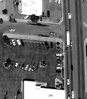
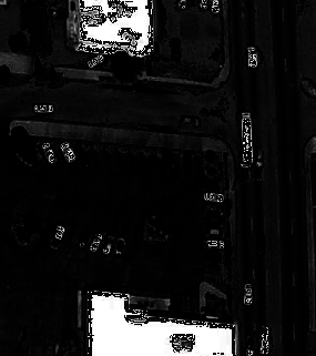
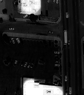
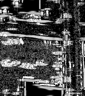
(a)	(b)	(c)	(d)	(e)

Figure 5: Subfigures (b)-(e) are five examples of features generated by a grammar and applied to the image shown in subfigure (a).

3.2 Pixel Classification with Spatially Exploitative AdaBoost

The top of Figure 2 illustrates the pixel classification part of the Beamer object detection pipeline. The goal of pixel classification is to fully delineate the class of interest but we introduce modifications. A set of feature extraction algorithms is applied to an image, resulting in a set of feature images. These feature images are thresholded and post-processed to create weak pixel classifiers for detecting object pixels. The final pixel classifier is a weighted combination of these weak pixel classifiers which output confidence with their predictions.

Learning is based on a training set where all the pixels belonging to the objects of interest (cars in our case) are hand-labeled. There are several difficulties in identifying good weak pixel classifiers from the hand-labeled training data. First, in applications like ours there are many more background pixels than foreground (object) pixels. Providing too much background puts too much emphasis on the background during learning, and can lead to hypotheses that do not perform well on the foreground. Second, hand-labeling is a subjective and error prone activity. Pixels outside the border of the object may be accidentally labeled as car, and pixels inside the border as background. It is well known that label noise causes difficulties for AdaBoost [Dietterich(2000), Rätsch et al.(2001)Rätsch, Onoda, and Müller]. This difficulty is compounded when the image data itself is noisy or there may not be sufficient information in a pixel neighborhood to correctly classify every pixel. Third, training a pixel classifier that fully segments is a much harder problem than localization. For example, if a weak hypothesis correctly labels only a tenth of the object pixels and these correct predictions are evenly distributed throughout the objects, the weak hypothesis will appear unfavorable. This is unfortunate because the weak hypothesis may be very good at localizing objects, just not fully segmenting them. Similarly, some otherwise good features may identify many objects as well as large swaths of background. In terms of localization, the performance is good but these hypotheses will be rejected by the learning algorithm because of the large number of false positives they produce.

We propose three spatially-motivated modifications to standard AdaBoost to perform well with the difficulties above. First, we weight the initial distribution so the sum of the foreground weight is proportionate with the background class. Second, we use confidence-rated AdaBoost proposed by Schapire and Singer [Schapire and Singer(1999)] so weak hypotheses can output low or zero confidence on pixels which may be noisy or labeled incorrectly. In confidence-rated boosting, the weak hypotheses output predictions from the real interval $[-1,1]$ and the more confident predictions are farther from zero. In the boosting literature, the edge is defined as the weighted training error. Third, we perform post-processing on the weak pixel classifications to improve those that produce good partial segmentations of objects.

Weak Classifier Post-processing

Four different weak pixel classification post-processing filters are considered and compared against no filtering at all. The first technique performs region growing (abbreviated R) with a 4-connected flood fill. Regions larger than $k$ pixels are identified and converted to abstentions (zero confidence predictions). This is useful for disambiguating cars from large swaths, such as buildings, which may have similar texture as cars. This simple post-processing filter works very well in practice. The other three post-processing techniques apply either an erosion (E), a dilation (D), or a local median filter (M) using a circular structuring element of radius $r$. When applying one of these filters, a pixel classifier only partially labeling an object will be evaluated more favorably. This improves the stability of learning in situations where the object pixels are noisy in the images and pixels are mislabeled. Section 4 thoroughly compares the performance of different combinations of these four post-processing filters, all of which show better performance than no filtering at all.

3.3 Learning and Predicting in the $(x,y)$ Location Domain

The final stage of object detection turns the confidence-rated pixel classification into a list of locations pointing to the objects in an image. Noisy and ambiguous data often reduce the quality of the pixel classification, but since we use pixel classification as a step along the way, we perform an extra round of training to learn to transform a rough labeling of object pixels into a high quality list of locality predictions, and to do so in a noise-robust and spatially exploitative manner. Pure pixel-based approaches are hard to optimize for location-based criteria, and often translate mislabeled pixels into false positives. Our algorithms turn the pixel classifications into a list of object locations, allowing us to operate in and directly optimize over the same domain as the output: a list of $(x,y)$ locations.

A confidence-rated pixel classification provides predictive power about which pixels are likely to belong to an object. The goal is a high quality localization, rather than object delineation, so we reduce the set of positive pixels to a smaller set of high-quality locations. The first object detector, Connected Components (CC) thresholds the confidence image at zero, performs binary dilation with a circular structuring element of radius $\sigma_{CC}$, finds connected components and marks detections at the centroids of the components.

Large Local Maxima (LLM), is like non-maximal suppression but instead represents the locations and magnitudes of the maxima in location space as opposed to image space. The approach sparsifies the set of high confidence pixels by including only local maxima as guesses of an object’s location. Next, the LLM detector chooses among the set of local maxima those pixel locations with confidences exceeding a threshold $\theta_{LLM}$. This method of detection is attractive because it is very fast, and somewhat reminiscent of decision stumps. The detector outputs these large maxima as its final predictions, ordering them with decreasing confidence. A Gaussian smoothing of width $\sigma_{LLM}$ can be applied before finding the maxima to reduce the noise and further refine the solutions.

The LLM detector treats maxima locations independently, which can be quite sensitive to the presence of outlier pixels and noisy imagery. Noisy imagery often leads to an excess of local maxima, some of which lie outside an object’s boundary, which often results in false positives. We propose an extension of the LLM detector called the Kernel Density Estimate (KDE) detector for combining maxima locations into a smaller, higher quality set of locations based on large numbers of maxima with high confidence clustered spatially close to one another. More specifically, the final detections are the modes of a confidence-weighted Kernel Density Estimate computed over the set of LLM locations. The width of the kernel is denoted $\sigma_{KDE}$. Our results show the KDE and LLM detectors perform remarkably well in the presence of noise.

4 Evaluation and Conclusions

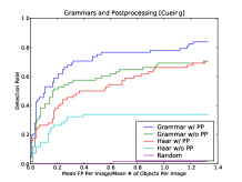
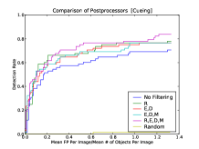
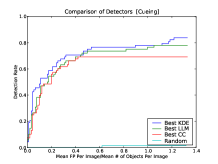
(a)	(b)	(c)
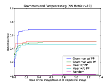
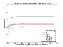
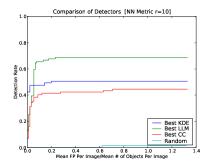
(d)	(e)	(f)

Figure 6: Subfigures (a-c) show the result of applying the best model to the validation set using the cueing metric. Subfigures (d-f) show the result for the nearest neighbors metric. The best model for each aspect in a comparison filter is applied to the unseen test data set.

Generating a ROC curve for a classifier involves marking each classification as a true negative or false positive. Quantifying the accuracy of unstructured object detection with a ROC curve is not as straightforward: the criteria for marking a true positive or false positive depends on the object detection task at hand. We consider three object detection problems: cueing, tracking, and counting and define two criteria to mark detections that are closely matched with these problems. Points on the ROC curves are then drawn using predicted locations above some confidence threshold.

Parameter	Parameters Tried
Iterations	$T\in\{10,25,50,75,100\}$
Features/per iter	$w=100$
Feature Set	Grammar, Haar-only, Grammar w/o Morphology or w/o Haar
Post-Processing	Region grow (R), Erosion (E), Dilation (D), Median (M), None (N)
	w/ combinations $\{R\}$, $\{E,D\}$, $\{E,D,M\}$, $\{R,E,D,M\}$, $\{N\}$
CC Detector	$\sigma_{CC}$ from 0 to 20 (0.2 increments) exclusive.
LLM Detector	$\sigma_{LLM}$ from 0 to 20 (0.2 increments) exclusive.
KDE Detector	$\sigma_{KDE}$ from 0 to 10 (0.1 increments) exclusive, $\sigma_{LLM}$ as above.
Features	Generate $w$ for each of $T$ iterations.
Decision Stump	Pick best threshold for each post-processing parameter tried.
Region grow PP	$k$ is varied from 1000 to 5000 (increments of 500).
Region grow PP	$k$ is varied from 1000 to 5000 (increments of 500).
E,D,M PP	$r$ is varied between $1$ and $5$.

Table 2: The first part of the table describes each parameter adjusted during validation. A highly extensive grid search was performed over a parameter space defined by the Cartesian product of these parameters. The second part shows the model parameters adjusted during an AdaBoost training iteration.

The goal of the cueing task is to output detections within the delineation of the object. False positives away from objects are penalized, but multiple true positives are not. Figure 6, subfigures (a-c) show the results for this metric.

We introduce the nearest neighbors criteria for marking detections for object tracking. Good detectors for tracking localize objects within some small error, and multiple detections of a given object are penalized. At each threshold the criteria finds the detection closest to an object. This pair is removed and the process is repeated until either no detections or no objects remain, or the distance of all remaining pairs exceeds a radius, $r$. Remaining objects are false negatives and remaining detections are false positives.

Lastly the task of object counting is concerned less with localization and more with accurate counts. We employ the nearest neighbors criteria for this purpose but to loosen the desire for a spatial correlation between detections and object locations, we set the nearest neighbor radius threshold $r$ to a high value.

We use the Area Under ROC Curve (AROC), computed numerically with the trapezoidal rule, as the statistic to optimize during validation to find the model parameters that perform the most favorably on the validation set. Since detectors may generate vast numbers of false positives, we arbitrarily truncate the curves at $U$ false positives per image ($U=30$ in our experiments). Validation is performed over the range of parameters given in Table 2.

Figure 6 illustrates the results of applying the most favorable models and parameter vectors (determined using the validation data) to the test set. Subfigure (a)–(c) and (d)–(f) illustrate the performance using the cueing and tracking metrics. Subfigures (a) and (d) show the clear advantage of using post-processing and grammar-guided features over just Haar-like features. Subfigure (b) and (e) show the benefit of post-processing for reducing the effects of label and image noise, and clearly highlights the need to properly tune parameters through validation and train all stages for each problem. Region growing performs better on the nearest neighbors metric–unsurprising as it abstains on ambiguous background patches, reducing false positives. On the cueing metric, morphology helps in reducing the effects of label noise, which often leads to false positives outside an object delineation. Finally subfigures (c) and (f) show that the spatially exploitative detection algorithms LLM and KDE outperform the pixel-based CC detector.

References

- [Agarwal et al.(2004)Agarwal, Awan, and Roth] Shivani Agarwal, Aatif Awan, and Dan Roth. Learning to Detect Objects in Images via a Sparse, Part-Based Representation. IEEE Transactions on Pattern Analysis and Machine Intelligence, pages 1475–1490, 2004.
- [Belongie et al.(2002)Belongie, Malik, and Puzicha] Serge Belongie, Jitendra Malik, and Jan Puzicha. Shape matching and object recognition using shape contexts. IEEE Transactions on Pattern Analysis and Machine Intelligence, 24:509–522, 2002.
- [Chum and Zisserman(2007)] Ondřej Chum and Andrew Zisserman. An exemplar model for learning object classes. IEEE Conference on Computer Vision and Pattern Recognition, pages 1–8, 2007.
- [Dietterich(2000)] Thomas G. Dietterich. An Experimental Comparison of Three Methods for Constructing Ensembles of Decision Trees: Bagging Boosting, and Randomization. Machine Learning, 40(2):139–157, 2000.
- [Dorkó and Schmid(2003)] Gyuri Dorkó and Cordelia Schmid. Selection of scale-invariant parts for object class recognition. IEEE International Conference on Computer Vision, 1:634, 2003.
- [Eads et al.(2005)Eads, Glocer, Perkins, and Theiler] Damian Eads, Karen Glocer, Simon Perkins, and James Theiler. Grammar-guided feature extraction for time series classification. Technical Report LA-UR-05-4487, Los Alamos National Laboratory, MS D436, Los Alamos, NM, 87545, June 2005.
- [Fergus et al.(2003)Fergus, Perona, and Zisserman] Rob Fergus, Pietro Perona, and Andrew Zisserman. Object class recognition by unsupervised scale-invariant learning. IEEE Conference on Computer Vision and Pattern Recognition, 2:264, 2003.
- [Ferrari et al.(2008)Ferrari, Fevrier, Jurie, and Schmid] Vittorio Ferrari, Loic Fevrier, Frédéric Jurie, and Cordelia Schmid. Groups of adjacent contour segments for object detection. IEEE Transactions on Pattern Analysis and Machine Intelligence, 30(1):36–51, January 2008.
- [Freund and Schapire(1996)] Yoav Freund and Robert E. Schapire. Experiments with a new boosting algorithm. In International Conference on Machine Learning, pages 148–156, 1996.
- [Heisele et al.(2003)Heisele, Ho, Wu, and Poggio] Bernd Heisele, Purdy Ho, Jane Wu, and Tomaso Poggio. Face recognition: component-based versus global approaches. Computer Vision and Image Understanding, 91(1-2):6–21, 2003.
- [Hopcroft and Ullman(1990)] John Hopcroft and Jeffrey Ullman. Introduction To Automata Theory, Languages, And Computation. Addison-Wesley, 1990.
- [Laptev(2006)] Ivan Laptev. Improvements of object detection using boosted histograms. British Machine Vision Conference, 3:949–958, 2006.
- [Lowe(1999)] David G. Lowe. Object recognition from local scale-invariant features. IEEE International Conference on Computer Vision, 2:1150, 1999.
- [Mikolajczyk et al.(2006)Mikolajczyk, Leibe, and Schiele] Kristian Mikolajczyk, Bastian Leibe, and Bernt Schiele. Multiple Object Class Detection with a Generative Model. Computer Vision and Pattern Recognition, pages 26–36, 2006.
- [Opelt et al.(2006)Opelt, Pinz, and Zisserman] Andreas Opelt, Axel Pinz, and Andrew Zisserman. A Boundary-Fragment-Model for Object Detection. Lecture Notes in Computer Science, 3952:575, 2006.
- [Papageorgiou et al.(1998)Papageorgiou, Oren, and Poggio] Constantine P. Papageorgiou, Michael Oren, and Tomaso Poggio. A general framework for object detection. IEEE International Conference on Computer Vision, pages 555–562, 1998.
- [Rätsch et al.(2001)Rätsch, Onoda, and Müller] Gunnar Rätsch, Takashi Onoda, and Klaus Müller. Soft margins for AdaBoost. Machine Learning, 42(3):287–320, 2001.
- [Schapire and Singer(1999)] Robert Schapire and Yoram Singer. Improved boosting algorithms using confidence-rated predictions. Machine Learning, 37(3):297–336, 1999.
- [Schneiderman and Kanade(2000)] Henry Schneiderman and Takeo Kanade. A statistical method for 3d object detection applied to faces and cars. IEEE Conference on Computer Vision and Pattern Recognition, page 1746, 2000.
- [Shotton et al.(2008)Shotton, Johnson, and Cipolla] Jamie Shotton, Matthew Johnson, and Roberto Cipolla. Semantic Texton Forests for Image Categorization and Segmentation. In IEEE Conference on Computer Vision and Pattern Recognition, pages 1–8, 2008.
- [Sipser(2005)] Michael Sipser. Introduction to the Theory of Computation. International Thomson Publishing, 2005.
- [Viola and Jones(2001)] Paul Viola and Michael Jones. Rapid object detection using a boosted cascade of simple features. Computer Vision and Pattern Recognition, IEEE Computer Society Conference on, 1:511, 2001.
- [Zhang et al.(2007)Zhang, Marszalek, Lazebnik, and Schmid] Jianguo Zhang, Marcin Marszalek, Svetlana Lazebnik, and Cordelia Schmid. Local features and kernels for classification of texture and object categories: A comprehensive study. International Journal of Computer Vision, 73(2):213–238, 2007.