Self-Organization of Balanced Nodes in Random Networks with Transportation Bandwidths

Abstract

We apply statistical physics to study the task of resource allocation in random networks with limited bandwidths along the transportation links. The mean-field approach is applicable when the connectivity is sufficiently high. It allows us to derive the resource shortage of a node as a well-defined function of its capacity. For networks with uniformly high connectivity, an efficient profile of the allocated resources is obtained, which exhibits features similar to the Maxwell construction. These results have good agreements with simulations, where nodes self-organize to balance their shortages, forming extensive clusters of nodes interconnected by unsaturated links. The deviations from the mean-field analyses show that nodes are likely to be rich in the locality of gifted neighbors. In scale-free networks, hubs make sacrifice for enhanced balancing of nodes with low connectivity.

1 Introduction

Analytical techniques developed in statistical physics have been widely employed in the analysis of complex systems in a wide variety of fields, such as neural networks hertz ; nishimori , econophysical models challet , and error-correcting codes nishimori ; kabashima . Recently, a statistical physics perspective was successfully applied to the problem of resource allocation on sparse random networks wong2006 ; wong2007 ; yeung2009b . Resource allocation is a well known network problem in the areas of computer science and operations management peterson ; ho . It is relevant to applications such as load balancing in computer networks, reducing Internet traffic congestion, and streamlining network flow of commodities shenker ; rardin .

In networks with finite bandwidths, the problem of resource allocation was studied in yeung2009 . We derived an algorithm which enable us to find the optimal solutions without the need of a global optimizer. The mean-field approach was applicable when the connectivity is sufficiently high. It allows us to derive the resource shortage of a node as a well-defined function of its capacity, which corresponds to the optimized and initial resource relation. For networks with uniformly high connectivity we derived the profile of the allocated resources which exhibits features similar to the Maxwell construction. We generalized the analysis to networks with arbitrary connectivity and compared the modified Maxwell construction with numerical solutions.

In this paper, we focus on the self-organization of nodes in achieving a balanced environment. The analytical results are compared with simulations, where nodes self-organize to balance their shortages. After defining the model in Section 2, we introduce the chemical potentials in Section 3. In Section 4 we review the theory of the Maxwell construction, which forms the basis for predicting the existence of clusters of balanced nodes. The emergence of balanced nodes correspond to the success in the uniform allocation of resources. We compare in Section 5.1 the statistics of saturated and unsaturated links, and show the existence of extensive balanced clusters. The deviations of the simulation results from the mean-field analyses show the dependence of final state on the locality of gifted and ungifted clusters in Section 5.2. We compare in Section 6 the fraction of balanced nodes in scale-free and regular networks and examine the role of hubs in resource allocation.

2 The Model

We consider a network with $N$ nodes, labelled $i\!=\!1,\dots,N$. Each node $i$ is randomly connected to $c$ other nodes. The connectivity matrix is given by ${\cal A}_{ij}=1,0$ for connected and unconnected node pairs respectively. Each node $i$ has a capacity $\Lambda_{i}$ randomly drawn from a distribution $\rho(\Lambda_{i})$. Positive and negative values of $\Lambda_{i}$ correspond to supply and demand of resources respectively. The task of resource allocation involves transporting resources between nodes such that the demands of the nodes can be satisfied to the largest extent. Hence we assign $y_{ij}\equiv-y_{ji}$ to be the current drawn from node $j$ to $i$, aiming at reducing the shortage $\xi_{i}$ of node $i$ defined by

$$\xi_{i}=\max\biggl{(}-\Lambda_{i}-\sum_{(ij)}{\cal A}_{ij}y_{ij},0\biggr{)}.$$ (1)

The magnitudes of the currents are bounded by the bandwidth $W$, i.e., $|y_{ij}|\leq W$.

To minimize the shortage of resources after their allocation, we include in the total cost both the shortage cost and the transportation cost. Hence, the general cost function of the system can be written as

$$E=R\sum_{(ij)}{\cal A}_{ij}\phi(y_{ij})+\sum_{i}\psi(\Lambda_{i},\{y_{ij}|{\cal A}_{ij}=1\}).$$ (2)

The summation $(ij)$ corresponds to summation over all node pairs, and $\Lambda_{i}$ is a quenched variable defined on node $i$.

In the present model of resource allocation, the first and second terms correspond to the transportation and shortage costs respectively. The parameter $R$ corresponds to the resistance on the currents, and $\Lambda_{i}$ is the capacity of node $i$. The transportation cost $\phi(y_{ij})$ can be a general even function of $y_{ij}$. In this paper, we consider $\phi$ and $\psi$ to be concave functions of their arguments, that is, $\phi^{\prime}(y)$ and $\psi^{\prime}(\xi)$ are non-decreasing functions. Specifically, we have the quadratic transportation cost $\phi(y)=y^{2}/2$, and the quadratic shortage cost $\psi(\Lambda_{i},\{y_{ij}|{\cal A}_{ij}=1\})=\xi_{i}^{2}/2$.

3 The Chemical Potentials and the Final Resources

The optimization problem can be written as the minimization of Eq. (2) in the space of $y_{ij}$ and $\xi_{i}$, subject to the constraints

$$\Lambda_{i}+\sum_{(ij)}{\cal A}_{ij}y_{ij}+\xi_{i}\geq 0,\quad\quad\xi_{i}\geq 0,$$ (3)

and the constraints on the bandwidths of the links $|y_{ij}|\leq W$. Introducing Lagrange multipliers to the above inequality constraints with the Kuhn-Tucker condition, the function to be minimized becomes

$$L\!=\!\sum_{i}\biggl{[}\psi(\xi_{i})+\mu_{i}\biggl{(}\Lambda_{i}+\sum_{(ij)}{\cal A}_{ij}y_{ij}+\xi_{i}\biggr{)}+\alpha_{i}\xi_{i}\biggr{]}$$

$$+\sum_{(ij)}{\cal A}_{ij}\biggl{[}R\phi(y_{ij})+\gamma^{+}_{ij}(W-y_{ij})+\gamma^{-}_{ij}(W+y_{ij})\biggr{]},$$ (4)

where $\mu_{i}\leq 0$, $\alpha_{i}\leq 0$, $\gamma_{ij}^{+}\leq 0$ and $\gamma_{ij}^{-}\leq 0$. Optimizing $L$ with respect to $y_{ij}$, one obtains

$$y_{ij}=Y(\mu_{j}-\mu_{i})$$ (5)

with

$$Y(x)=\max\biggl{\{}-W,\min\biggl{[}W,[\phi^{\prime}]^{-1}\biggl{(}\frac{x}{R}\biggr{)}\biggr{]}\biggr{\}}.$$ (6)

The Lagrange multiplier $\mu_{i}$ is referred to as the chemical potential of node $i$, and $\phi^{\prime}$ is the derivative of $\phi$ with respect to its argument. The function $Y(\mu_{j}-\mu_{i})$ relates the potential difference between nodes $i$ and $j$ to the current driven from node $j$ to $i$. For the quadratic cost, it consists of a linear segment between $\mu_{j}-\mu_{i}=\pm WR$ reminiscent of Ohm’s law in electric circuits. Beyond this range, $y$ is bounded above and below by $\pm W$ respectively. Thus, obtaining the optimized configuration of currents $y_{ij}$ among the nodes is equivalent to finding the corresponding set of chemical potentials $\mu_{i}$, from which the optimized $y_{ij}$’s are then derived from $Y(\mu_{j}-\mu_{i})$. This implies that we can consider the original optimization problem in the space of chemical potentials.

The optimal currents are given by Eq. (5) in terms of the chemical potentials $\mu_{i}$ which, from Eqs. (1) and (3), are related to their neighbors via

$$\mu_{i}=\begin{cases}0\qquad\qquad\qquad\mbox{ for $h_{i}^{-1}(0)>0$,}\\ h_{i}^{-1}(0)\qquad\qquad\mbox{ for $-\psi^{\prime}(0)\leq h_{i}^{-1}(0)\leq 0$,}\\ g_{i}^{-1}(0)\qquad\qquad\mbox{ for $h_{i}^{-1}(0)<-\psi^{\prime}(0)$,}\end{cases}$$

where $h_{i}(x)$ and $g_{i}(x)$ are given by

$$h_{i}(x) = -\Lambda_{i}-\sum_{j}{\cal A}_{ij}Y(\mu_{j}-x),$$

$$g_{i}(x) = \psi^{\prime}\circ h_{i}(x)+x,$$ (8)

with function $Y$ again given Eq. (6). $h_{i}(x)$ is the shortage of resource at node $i$ when $\mu_{i}$ takes the value $x$. $\psi^{\prime}\circ h_{i}(x)$ is then the corresponding dissatisfaction cost per unit resource of node $j$. For the quadratic shortage cost considered in this paper, the frictionless condition $\psi^{\prime}(0)=0$ is satisfied. Equation (3) is then simplified to

$$\mu_{i}=\min\left(0,-h_{i}(\mu_{i})\right).$$ (9)

Hence we can interpret $\mu_{i}$ as the final shortage of resources after optimization. When $\mu_{i}<0$, $-\mu_{i}$ becomes the final resources allocated to node $i$. Equation (9) provides a simple local iteration algorithm for the optimization problem in which the optimal currents can be evaluated from the potential differences of neighboring nodes.

An alternative algorithm can be obtained by adopting message-passing approaches, which have been successful in problems such as error-correcting codes opper2001 and probabilistic inference mackay2003 . We refer the interested readers to yeung2009 for a comprehensive derivation of the messages.

4 The Resource Distribution Profile

4.1 The High Connectivity Limit

We consider the case that the bandwidth of individual links scales as $\tilde{W}/c$ when the connectivity increases, where $\tilde{W}$ is a constant. Thus the total bandwidth $\tilde{W}$ available to an individual node remains a constant.

We start by writing the chemical potentials using Eq. (9),

$$\mu_{i}=\min\biggl{[}\Lambda_{i}+\sum_{j=1}^{N}{\cal A}_{ij}Y(\mu_{j}-\mu_{i}),0\biggr{]}.$$ (10)

In the high connectivity limit, the interaction of a node with all its connected neighbors become self-averaging, making it a function singly dependent on its own chemical potential, namely,

$$\sum_{j=1}^{N}{\cal A}_{ij}Y(\mu_{j}-\mu_{i})\approx cM(\mu_{i}).$$ (11)

Physically, the function $M(\mu)$ corresponds to the average interaction of a node with its neighbors when its chemical potential is $\mu$, facilitating a mean-field approach. Thus, we can write Eq. (10) as

$$\mu=\min[\Lambda+cM(\mu),0],$$ (12)

where $\mu$ is now a function of $\Lambda$, and

$$M(\mu_{i})=\int_{-\infty}^{\infty}d\Lambda\rho(\Lambda)Y(\mu(\Lambda)-\mu_{i})$$ (13)

where we have written the chemical potential of the neighbors as $\mu(\Lambda)$, assuming that they are well-defined functions of their capacities $\Lambda$.

To explicitly derive $M(\mu)$, we take advantage of the fact that the rescaled bandwidth, $\tilde{W}/c$ vanishes in the high connectivity limit, so that the current function $Y(\mu_{j}-\mu_{i})$ is effectively a sign function, corresponding to saturated links. (This approximation is not fully valid and will be further refined in subsequent discussions.) Thus, we approximate

$$M(\mu_{i})=\frac{\tilde{W}}{c}\int_{-\infty}^{\infty}d\Lambda\rho(\Lambda){\rm sgn}[\mu(\Lambda)-\mu_{i}].$$ (14)

Assuming that $\mu(\Lambda)$ is a monotonic function of $\Lambda$, and for Gaussian distribution of capacities, $\mu(\Lambda)$ is explicitly given by

$$\mu=\min\biggl{[}\Lambda-\tilde{W}{\rm erf}\biggl{(}\frac{\Lambda-\langle\Lambda\rangle}{\sqrt{2}}\biggr{)},0\biggr{]}.$$ (15)

This equation relates the chemical potential of a node, i.e. the shortage after resource allocation, to its initial resource before. It tells us that resource allocation through a large number of links results in a well-defined function relating the two quantities.

Eq. (15) gives a well-defined function $\mu(\Lambda)$ as long as $\tilde{W}\leq\sqrt{\pi/2}$. However, when $\tilde{W}>\sqrt{\pi/2}$, turning points exists in $\mu(\Lambda)$ as shown in Fig. 1(a). This creates a thermodynamically unstable scenario, since in the region of $\mu(\Lambda)$ with negative slope, nodes with lower capacities have higher chemical potentials than their neighbors with higher capacities. Mathematically, the non-monotonicity of $\mu(\Lambda)$ means that ${\rm sgn}[\mu(\Lambda)-\mu_{i}]$ and ${\rm sgn}(\Lambda-\Lambda_{i})$ are no longer necessarily equal, and Eq. (15) is no longer valid.

Figure 1: The Maxwell construction on $\mu(\Lambda)$.

Nevertheless, Eq. (10) permits another solution of constant $\mu$ in a range of $\Lambda$. Hence, we propose that the unstable region of $\mu(\Lambda)$ should be replaced by a range of constant $\mu$ as shown in Fig. 1(b) analogous to the Maxwell construction in thermodynamics. Nodes within this range of constant $\mu$ have the same amount of final resources, and is the consequence of the ability of the optimization process to balance the resources. They are referred to as the balanced nodes.

In the high connectivity limit, resources are so efficiently allocated that the resources of the rich nodes are maximally allocated to the poor nodes. By considering the conservation of resources, and letting $(\Lambda_{<},\mu_{o})$ and $(\Lambda_{>},\mu_{o})$ be the end points of the Maxwell construction as shown in Fig. 1(b), we have proved in yeung2009 that

$$\mu_{o}\int_{\Lambda_{<}}^{\Lambda_{>}}d\Lambda\rho(\Lambda)=\int_{\Lambda_{<}}^{\Lambda_{>}}d\Lambda\rho(\Lambda)\mu(\Lambda),$$ (16)

which implies that the value of $\mu_{o}$ should be chosen such that the areas A and B in Fig. 1(b), weighted by the distribution $\rho(\Lambda)$, should be equal.

For capacity distributions $\rho(\Lambda)$ symmetric with respect to $\langle\Lambda\rangle$, we have $\mu_{o}=\langle\Lambda\rangle=(\Lambda_{<}+\Lambda_{>})/2$. As a result, the function $\mu(\Lambda)$ is given by

$$\mu(\Lambda)=\begin{cases}\langle\Lambda\rangle\qquad\qquad\qquad\qquad\mbox{ for $\Lambda_{<}<\Lambda<\Lambda_{>}$,}\\ \\ \min\left[\Lambda-\tilde{W}{\rm erf}\left(\frac{\Lambda-\langle\Lambda\rangle}{\sqrt{2}}\right),0\right]\mbox{ otherwise,}\\ \end{cases}$$ (17)

where as $\Lambda_{<}$ and $\Lambda_{>}$ are respectively given by the lesser and greater roots of the equation $x=\langle\Lambda\rangle+\tilde{W}{\rm erf}[(x-\langle\Lambda\rangle)/\sqrt{2}]$.

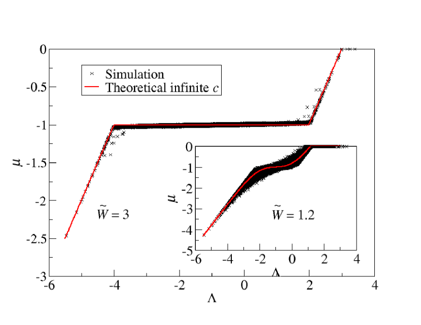
Figure 2: The simulation results of $\mu(\Lambda)$ for $N=10000$, $c=15$, $R=0.1$, $\langle\Lambda\rangle=-1$ and $\tilde{W}=3$ with 70000 data points, compared with theoretical prediction. Inset: The corresponding results for $\tilde{W}=1.2$.

We compare the analytical result of $\mu(\Lambda)$ in Eq. (17) with simulations in Fig. 2. For $\tilde{W}>\sqrt{\pi/2}$, data points $(\Lambda,\mu)$ of individual nodes from network simulations follow the analytical result of $\mu(\Lambda)$, giving an almost perfect overlap of data. The presence of the balanced nodes with effectively constant chemical potentials is obvious and essential to explain the behavior of the majority of data points from simulations. On the other hand, for $\tilde{W}<\sqrt{\pi/2}$, the analytical $\mu(\Lambda)$ shows no turning point as shown in the inset of Fig. 2. Despite the scattering of data points, they generally follow the trend of the theoretical $\mu(\Lambda)$.

4.2 The Cases with General Connectivity

Our analysis can be generalized to the case of large but finite connectivity, where the approximation in Eq. (14) is not fully valid. This modifies the chemical potentials of the balanced nodes, for which Eq. (14) has to be replaced by

$$M(\mu) =\frac{\tilde{W}}{c}\biggl{[}\int_{\Lambda_{>}}^{\infty}d\Lambda\rho(\Lambda)-\int_{-\infty}^{\Lambda_{<}}d\Lambda\rho(\Lambda)\biggr{]}$$ (18)

$$+\int_{\Lambda_{<}}^{\Lambda_{>}}d\Lambda\rho(\Lambda)\biggl{(}\frac{\mu(\Lambda)-\mu}{R}\biggr{)}.$$

We introduce an ansatz of a linear relationship between $\mu$ and $\Lambda$ for the balanced nodes, namely,

$$\mu=m\Lambda+b.$$ (19)

After direct substitution of Eq. (19) into $M(\mu)$ given by Eq. (18), we get the self-consistent equations for $m$ and $b$,

$$m=\frac{R}{R+c~{}{\rm erf}\left(\frac{\Lambda_{>}-\langle\Lambda\rangle}{\sqrt{2}}\right)},$$

$$b=\frac{c~{}{\rm erf}\left(\frac{\Lambda_{>}-\langle\Lambda\rangle}{\sqrt{2}}\right)}{R+c~{}{\rm erf}\left(\frac{\Lambda_{>}-\langle\Lambda\rangle}{\sqrt{2}}\right)}\langle\Lambda\rangle.$$ (20)

Thus, the Maxwell construction has a non-zero slope when the connectivity is finite.

We remark that the approximation in Eq. (18) assumes that the potential differences of the balanced nodes lie in the range of $2R\tilde{W}/c$, so that their connecting links remain unsaturated. Note that the end points of the Maxwell construction have chemical potentials $\langle\Lambda\rangle\pm R\tilde{W}/c$ respectively, rendering the approximation in Eq. (18) exact at one special point, namely, the central point of the Maxwell construction. Hence, this approximation works well in the central region of the Maxwell construction, while deviations are expected near the end points.

We compare Eq. (18) with the $\mu(\Lambda)$ given by the numerical solution of the integral equation

$$\mu(\Lambda_{i})=\Lambda_{i}+\int_{-\infty}^{\infty}d\Lambda\rho(\Lambda)Y[\mu(\Lambda)-\mu(\Lambda_{i})].$$ (21)

Since iterating this equation may lead to an oscillating solution of $\mu(\Lambda)$, we solve it by gradient descent. The results are shown in Fig. 3 in an enlarged scale of $\mu$. As expected, Eq. (18) works well around $\mu=\langle\Lambda\rangle$ and show small deviations at the end points of the Maxwell construction. In comparison with simulations, data porints are scattered from the theoretical predictions, but generally follow the slanted path of $\mu(\Lambda)$ rather than the horizontal path as predicted by Eq. (17). We will explain the scattering of data points in the next section. As shown in the inset of Fig. 3, the differences among the different approaches are not obvious unless the scale of $\mu$ is expanded. We thus conclude that both the horizontal and slanted Maxwell constructions are good approximations of $\mu(\Lambda)$ and capture the general trend of the simulation data.

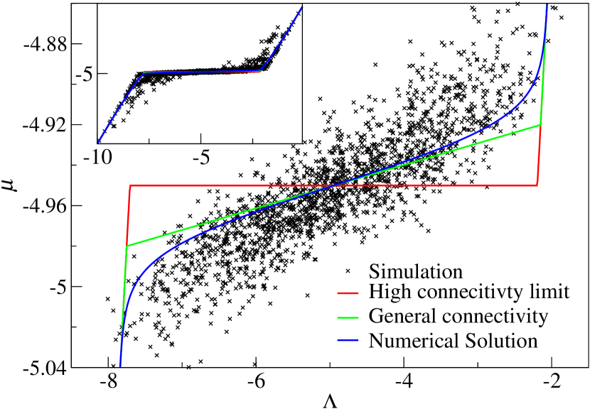
Figure 3: Simulation results of $(\Lambda,\mu)$ for $N=2000$, $\tilde{W}=3$, $c=10$ and $\langle\Lambda\rangle=-5$ shown with an expanded vertical scale, as compared with the theoretical predictions of $\mu(\Lambda)$ from Eq. (17), Eq. (18) and the numerical solution of Eq. (21). Inset: same data set and theoretical predictions in the normal vertical scale.

Remarkably, as evident from Eq. (4.2), even with constant available bandwidth $\tilde{W}$, increasing connectivity causes $m$ to decrease, and hence sharpens the chemical potential distribution. The narrower distributions correspond to higher efficiency in resource allocation. It leads us to realize the potential benefits of increasing connectivity in network optimization even for a given constant total bandwidth connecting a node.

5 The Self-organization of the Balanced Nodes

The fraction $f_{\rm bal}$ of balanced nodes is given by the equation

$$f_{\rm bal}={\rm erf}\biggl{(}\frac{\tilde{W}f_{\rm bal}}{\sqrt{2}}\biggl{)}.$$ (22)

Note that $f_{\rm bal}$ has the same dependence on $\tilde{W}$ for all negative $\langle\Lambda\rangle$. Figure 4 shows that when the total bandwidth $\tilde{W}$ increases beyond $\sqrt{\pi/2}$, the analytical fraction of balanced nodes increases, reflecting the more efficient resource allocation brought by the convenience of increased bandwidths. When $\tilde{W}$ becomes very large, a uniform chemical potential of $\langle\Lambda\rangle$ networkwide is recovered. converging to the case of non-vanishing bandwidths yeung2009 .

Figure 4: Analytical predictions of $f_{\rm bal}$ as compared with simulation results for networks of $N=10000$, $\tilde{W}=3$, $R=0.1$ and $\langle\Lambda\rangle=-5$.

We measure $f_{\rm bal}$ in simulations as follows. As only finite connectivity can be implemented, we define node $i$ to be balanced when its chemical potential falls into the slanted range of the Maxwell construction, i.e. $\langle\Lambda\rangle-R\tilde{W}/c\leq\mu_{i}\leq\langle\Lambda\rangle+R\tilde{W}/c$. The simulation results are compared with the analytical results in Fig. 4. Deviations are found at intermediate values of $\tilde{W}$, which may be expained by the scattering of simulated data points. Nevertheless, increass in $f_{\rm bal}$ are observed at $\tilde{W}\approx\sqrt{\pi/2}$, corresponding to the emergence of balanced nodes in simulations.

5.1 The Extensive Clusters of Balanced Nodes

In random networks, balanced nodes are found in clusters interconnected by an extensive fraction of unsaturated links. The clusters connect most balanced nodes and span the whole network when a large fraction of balanced node is found. The unsaturated links in the clusters provide the freedom to fine tune their currents so that the shortages among the nodes are uniform. These features are the natural consequences of optimization, in which nodes self-organize to balance their shortages.

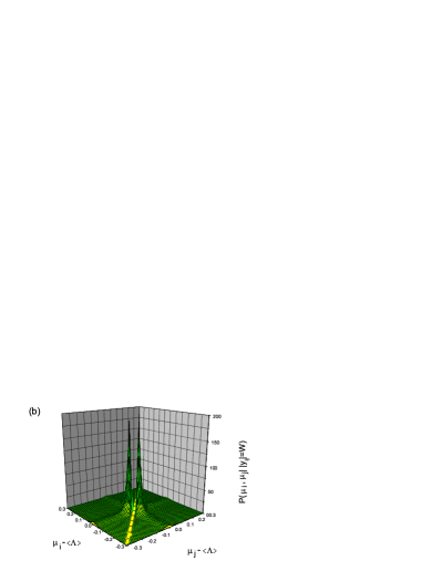
Figure 5: The distributions (a) $P(\mu_{i},\mu_{j}||y_{ij}|<W)$ and (b) $P(\mu_{i},\mu_{j}||y_{ij}|=W)$, corresponding to the joint probability distributions of the final resources of terminal nodes $i$ and $j$ for link $(ij)$, given the link is unsaturated and saturated respectively. Parameters: $N=10000$, $\tilde{W}=3$, $R=0.1$ and $\langle\Lambda\rangle=-5$.

To examine the clustering of balanced nodes, we show in Fig. 5 (a) and (b) respectively the distributions $P(\mu_{i},\mu_{j}||y_{ij}|<W)$ and $P(\mu_{i},\mu_{j}||y_{ij}|=W)$, which correspond to the joint probability distributions of the final resources of terminal nodes $i$ and $j$ for link $(ij)$, given the link is unsaturated and saturated. As shown in Fig. 5 (a), unsaturated links connect nodes with $\mu_{i}\approx\mu_{j}$. A prominent peak is found around $\mu_{i}\approx\mu_{j}\approx\langle\Lambda\rangle$, corresponding to unsaturated linkages between the balanced nodes. On the other hand, $P(\mu_{i},\mu_{j}||y_{ij}|=W)$ shows non-zero probabilities in regions other than $\mu_{i}\approx\mu_{j}$. Peaks are observed, which are similar to a Gaussian distribution with the central slice removed. Non-zero probabilities are observed along the axes $\mu_{i}\approx\langle\Lambda\rangle$ and $\mu_{j}\approx\langle\Lambda\rangle$, corresponding to saturated linkages between balanced and unbalanced nodes. These results support the existence of balanced clusters interconnected by an extensive fraction of unsaturated links.

5.2 The Neighborhood of Rich and Poor Nodes

To understand the scattering of data points of $(\mu,\Lambda)$ from the mean-field predictions, we identify the role of the nodes in resource allocation according to their capacities. Nodes with capacities greater and less than $\langle\Lambda\rangle$ are respectively referred to as the gifted and ungifted nodes. Figure 6 shows the schematic relation of the resources of a node before and after optimization. Before optimization, the resource of a node is equal to its capacity. After optimization, the resource of a node is equal to $\mu$. Gifted nodes have their resources reduced after donating them, and ungifted nodes have their resources increased after receiving them. $\mu(\Lambda)$ is then described by the Maxwell construction as derived in the mean-field analysis.

Figure 6: The schematic relation of the resources of a node (a) before and (b) after optimization. The division of nodes into gifted rich, gifted poor, ungifted rich and ungifted poor is shown in (b).

As finite connectivity is implemented in simulations, the neighborhood of a node deviates from the mean-field descriptions which results in scattering of data points $(\mu,\Lambda)$. To examine the effect of the locality of nodes in relation with their final shortage, we define rich and poor nodes to be nodes with final resources higher and lower than the mean-field predictions. As shown in Fig. 6(b), the nodes are thus categorized into gifted rich, gifted poor, ungifted rich and ungifted poor, in accordance to the scattering of the capacity-shortage relations i.e. $(\mu,\Lambda)$ of the node. As an example, gifted rich nodes are nodes with initial capacity higher than $\langle\Lambda\rangle$ and final resources higher than the mean-field predictions, as shown in Fig. 6(b).

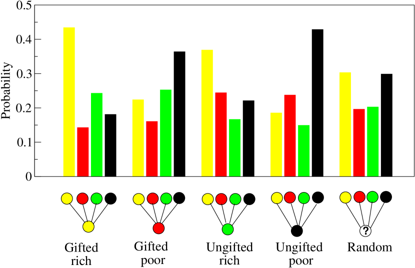
Figure 7: The fraction of gifted rich, gifted poor, ungifted rich and ungifted poor nodes among the nearest neighbors of a node in a particular category. Parameters: $N=10000$, $\tilde{W}=3$, $R=0.1$, $\langle\Lambda\rangle=-5$ and 5 samples.

We examine the neighborhood of a node in Fig. 7 by measuring the fractions of gifted rich, gifted poor, ungifted rich and ungifted poor nodes among its nearest neighbors. As compared with the random case, a high ratio of gifted rich node is found surrounding a gifted rich node. In other words, gifted nodes are more likely to be rich in the neighborhood of gifted nodes, forming a cluster of rich nodes after allocation. Physically, the effective average capacity is higher than $\langle\Lambda\rangle$ in the locality of gifted clusters, leading to higher resources than the mean-field predictions. The converse is true for ungifted poor nodes, which results in lower resources in the locality of ungifted clusters. On the other hand, gifted nodes are more likely to be poor if they are in the neighborhood of ungifted clusters, as shown by the statistics of the neighbors of gifted poor nodes, and vice versa. We thus conclude that the final state of a node is highly dependent on its locality, which results in the scattering of the simulated data points of $(\mu,\Lambda)$ around the prediction of the mean-field analyses.

6 Balanced Nodes in Scale-Free Networks

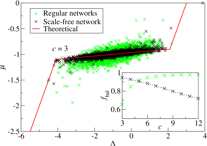
Figure 8: Simulation results of $(\Lambda,\mu)$ for networks of $N=2\times 10^{5}$, $\tilde{W}=3$, $R=0.1$ and $\langle\Lambda\rangle=-1$ with uniform connectivity of $c=3$ and scale-free network of $P(c)\sim c^{-3}$ with $c\geq 3$, each with 2500 data points, as compared with the theoretical predictions of Eq. (4.2). Inset: the $f_{\rm bal}$ as a function of $c$ for nodes in scale-free and regular networks with N=10000 and 50 samples.

We have examined the features of balanced nodes in regular networks . However, recent studies of complex networks show that many realistic communication networks have highly heterogeneous structure, and the connectivity distribution obeys a power law barabasi . These networks, commonly known as scale-free networks, are characterized by the presence of hubs, which are nodes with very high connectivities, and are found to modify the network behavior significantly. Hence, it is interesting to study the allocation of resources and the features of balanced nodes in scale-free networks. We define the bandwidth of the link $(ij)$ to be $W_{ij}=\tilde{W}/\max(c_{i},c_{j})$, where $c_{i}$ and $c_{j}$ are the connectivity of the terminal nodes. In this case, nodes in scale-free network may have a smaller effective $\tilde{W}$, as compared with their counterpart in regular networks with identical connectivity.

The simulation results are presented in Fig. 8, where we plot the data points of $(\Lambda,\mu)$ from nodes of $c=3$ in scale-free networks. Despite their low connectivity, their capacity-shortage relations exhibit the flat distribution characteristic of the Maxwell construction, coinciding with the analytical results of the high connectivity limit. This shows that the presence of hubs in scale-free networks increases the global efficiency of resource allocation, leading to balanced shortages on nodes with low connectivity. To confirm this advantage of the scale-free topology, we also plot in the figure the data points obtained from networks of uniform connectivity $c=3$. Evidently, the data points are much more scattered away from the Maxwell construction.

However, the enhanced balancing in scale-free networks are found only for nodes with low connectivity. We compare in the inset of Fig. 8, the $f_{\rm bal}$ in scale-free networks and regular networks, for nodes with higher connectivities. From the firgure for $c=3,4$, a much higher $f_{\rm bal}$ is found in scale-free networks than their counterparts in regular networks. The opposite is true for $c\geq 5$, and the differences increases with $c$. It implies that the nodes with higher connectivity in scale-free neworks sacrifice themselves for balancing the majority of nodes with low connectivity. In contrast, the fraction of balanced nodes increases with the connectivity in regular networks. This picture thus clarifies the role of hubs in resource allocation on scale-free networks.

7 Conclusion

We have applied statistical mechanics to study an optimization task of resource allocation on a network, in which nodes with different capacities are connected by links of finite bandwidths. By adopting suitable cost functions, such as quadratic transportation and shortage costs, the model can be applied to the study of realistic networks. The mean-field approach valid in the high connectivity limit enables us to derive the capacity-shortage relations, and study the deviations from this limit for finite connecitivty.

In particular, the study reveals interesting effects due to finite bandwidths. A remarkable phenomenon is found in networks with fixed total bandwidths per node, where bandwidths per link vanish in the high connectivity limit. For sufficiently large total bandwidths, clusters of balanced nodes self-organize to have a uniform shortage reminiscent of the Maxwell construction in thermodynamics. The locality of gifted and ungifted clusters respectively lead to the formation of rich and poor clusters. In scale-free networks, hubs are more likely to be unbalanced and make sacrifice for nodes with low connectivity to get balanced. We believe that the present analyses of balanced nodes lead us to better understanding of self-organization in resource allocation, as well as other systems.

References

- (1) J. Hertz, A. Krogh, and R. G. Palmer, Introduction to the Theory of Neural Computation (Addison-Wesley, Redwood City, 1991).
- (2) H. Nishimori, Statistical Physics of Spin Glasses and Information Processing (Oxford University Press, Oxford, UK, 2001).
- (3) D. Challet, M. Marsili and Y.-C. Zhang Minority Games (Oxford University Press, Oxford, UK, 2005).
- (4) Y. Kabashima and D. Saad, J. Phys. A 37, R1 (2004).
- (5) K. Y .M. Wong and D. Saad, Phys. Rev. E 74, 010104(R) (2006).
- (6) K. Y .M. Wong and D. Saad, Phys. Rev. E 76, 011115 (2007).
- (7) C. H. Yeung and K. Y. M. Wong, to appear in Phys. Rev E (2009).
- (8) L. Peterson and B.S. Davie, Computer Networks: A Systems Approach (Academic Press, San Diego CA, 2000).
- (9) Y. C. Ho, L. Servi, and R. Suri, Large Scale Syst. 1, 51 (1980).
- (10) S. Shenker, D. Clark, D. Estrin and S. Herzog, Comput. Commun. Rev. 26. 19 (1996).
- (11) R. L. Rardin Optimization in Operations Research (Prentice Hall, Englewood Cliffs, NJ, 1998).
- (12) C. H. Yeung and K. Y. M. Wong J. Stat. Mech. P03029 (2009).
- (13) M. Mézard, G. Parissi and M. A. Virasoro Spin Glass Theory and Beyond (World Scientific, 1987).
- (14) M. Opper and D. Saad, eds, Advanced Mean Field Methods (MIT Press, Cambridge, MA, 1999).
- (15) D. J. C. Mackey, Information Theory, Inference and Learning Algorithms (Cambridge University Press, UK, 2003).
- (16) A. L. Barabási and R. Albert, Science 286, 509 (1999).