Non-Markovian dissipative dynamics of two coupled qubits in independent reservoirs:
a comparison between exact solutions and master equation approaches

Abstract

The reduced dynamics of two interacting qubits coupled to two independent bosonic baths is investigated. The one-excitation dynamics is derived and compared with that based on the resolution of appropriate non-Markovian master equations. The Nakajima-Zwanzig and the time-convolutionless projection operator techniques are exploited to provide a description of the non-Markovian features of the dynamics of the two-qubits system. The validity of such approximate methods and their range of validity in correspondence to different choices of the parameters describing the system are brought to light.

I Introduction

Despite its simplicity a two-state system is of great significance being it exploitable to effectively describe many real situations. The theoretical analysis as well as the practical implementation of interacting or not two-level systems thus represents a central topic in several branches of modern physics ranging from high energy to nuclear and condensed matter physics polyakov ; belitsky . During the last decade the interest towards two-level systems has further been stimulated by the fact that a qubit represents the basic element in the context of the new applicative area of quantum information and communication. It has been for example shown that a fundamental quantum gate like the C-NOT gate can be implemented using dipole-dipole interacting quantum dots modeled as two qubits baranco . Moreover due to the development of new technologies, today there are several possible routes to the creation of what might be termed quantum bit, each based on a different physical system. These include quantum optics, microscopic quantum objects (electrons, ions, atoms) in traps, quantum dots and quantum circuits amico ; 6 ; 7 ; 8 ; 9 ; 10 ; bellomo ; garraway1 ; garraway2 ; garraway4 . In describing real systems however it is mandatory to take into account the effects stemming from the presence of the surroundings. Thus the dissipative dynamics of two-level systems has been the subject of numerous papers appeared in literature in the last decades agarwal ; sinaysky ; quiroga ; maniscalco ; Mazzola ; yu ; scala . Generally speaking the research has been developed assuming a Markovian environment agarwal ; sinaysky . But memory effects are in general present and could affect quantitatively and qualitatively the dynamics of the small system. Unfortunately, there are no fully systematic investigations of non-Markovian environments. Projection operator techniques, such as the time-convolutionless (TCL) Chaturvedi and the Nakajima-Zwanzig (NZ) Nakajima ; Zwanzig approaches, are in general exploited in order to perform a description of the non-Markovian features of the dynamics of open systems. On the one hand, the NZ provides a generalized master equation in which the time derivative of the density operator is connected to the past history of the state through the convolution of the density operator and an appropriate integral kernel. On the other hand the TCL approach provides a generalized master equation which is local in time. Intuitively, one might argue that the NZ should work better than the TCL approach in describing the memory effect, since it explicitly takes into account the past history of the open system. Anyway there are examples in which the exact dynamics of the open system can be described by means of a master equation which is local in time, as in the well known case of the Hu-Paz-Zhang generalized master equation for the non-Markovian theory of quantum Brownian motion hu ; petruccionebook .

In general it is not easy to establish whether one method is better than the other one. In fact, the performance of these perturbation schemes strongly depends on the details of the system under investigation. In this paper we consider two interacting two-level systems, each coupled to its own bosonic bath, exactly solving their dynamics in a one excitation subspace. The knowledge of the exact dynamics is exploited to test perturbative approaches based on TCL and NZ techniques. We show that, counterintuitively, the TCL approach works better than the NZ one, since the latter approach does not guarantee the positivity of the density matrix when the correlations inside the reservoir become moderately strong. On the contrary the TCL approach describes all the qualitative features of non-Markovian dynamics for a wider range of values of reservoir memory time.

The paper is organized as follows. In Sec. II we derive the exact equations governing the evolution of the two-qubit system coupled to two independent reservoirs, in the case of one initial excitation, and find their exact solution. In Sec. III the derivation of the second order NZ equation is presented and the features of the second order TCL, derived in Ref.Ferraro , are recalled. An extensive comparison among the exact, the NZ and the TCL is presented in Sec. IV, while in Sec. V some conclusive remarks are given.

II Exact dynamics

II.1 The model

The physical system on which we focus our attention is composed by two interacting two-level systems. Each qubit is moreover coupled to an external environment modeled as a bosonic bath quiroga . Assuming $\hbar=1$, the Hamiltonian model describing the total system can be written in the following form

$$H=H_{0}+H_{I}.$$ (1)

Here

$$H_{0}=\frac{\omega_{0}}{2}\sigma_{z}^{(1)}+\frac{\omega_{0}}{2}\sigma_{z}^{(2)}+\sum_{j=1,2}\sum_{k}\omega_{k}^{(j)}b_{k}^{(j)\dagger}b_{k}^{(j)}$$ (2)

is the unperturbed part containing the free Hamiltonian of the two qubits as well as that of the two independent environments. The transition frequency of the two two-level systems, supposed coincident for simplicity, is indicated by $\omega_{0}$ whereas $\sigma_{z}^{(j)}$ ($j=1,2$) denotes the Pauli operator describing the $j$-th subsystem. The two independent bosonic baths are characterized by proper frequencies $\omega_{k}^{(j)}$, $b_{k}^{(j)\dagger}$ and $b_{k}^{(j)}$ being correspondingly the creation and annihilation bosonic operators.

The interaction term

$$\begin{split}H_{I}=&\Omega(\sigma_{+}^{(1)}\sigma_{-}^{(2)}+\sigma_{-}^{(1)}\sigma_{+}^{(2)})+\\ &+\sum_{j=1,2}\left(\sigma_{+}^{(j)}\sum_{k}g_{k}^{(j)}b_{k}^{(j)}+\sigma_{-}^{(j)}\sum_{k}g_{k}^{(j)\ast}b_{k}^{(j)\dagger}\right)\end{split}$$ (3)

includes both the direct interaction between the two qubits, characterized by the coupling constant $\Omega$, and the interaction between each qubit and its respective bosonic bath, with coupling constants $g_{k}^{(j)}$. In eq.(3) $\sigma_{\pm}^{(j)}\equiv\frac{1}{2}(\sigma_{x}^{(j)}\pm i\sigma_{y}^{(j)})$ are, as usual, the lowering and raising Pauli operators.

It is worth underlining that the Hamiltonian model (1) is quite versatile in the sense that it can be successfully adopted to describe many different physical systems. In the framework of cavity QED bellomo or circuit QED 6 ; 7 ; 8 ; 9 ; 10 this model can be indeed exploited for the description of two atoms in spatially separated cavities as well as of two far enough Josephson charge, flux or phase qubits so that it is reasonable to assume that they interact with two different electromagnetic environments. Model (1) in addition allows to study the influence of spurious microwave resonators within Josephson tunnel junctions on the coherent dynamics of a phase qubit martinis . In this case the environment coupled to the spurious resonator (modeled as a two state system) is a phononic bath.

Very recently the Markovian dynamics stemming from Hamiltonian (1) has been analyzed sinaysky . In Ref.Ferraro instead the TCL approach has been exploited in order to investigate on the non-Markovian regime. In this paper we exactly solve the time-dependent Schrödinger equation confining ourselves to the one excitation subspace. At the same time we adopt the NZ technique to derive a non-Markovian master equation for the reduced density operator of the two coupled qubits. Having at our disposal both the exact dynamics and the approximate master equations, a comparison may be done in order to test the effectiveness of the perturbative approaches. From now on, we work in the interaction picture defined by $H_{0}$ in which the interaction Hamiltonian reads

$$H_{I}(t)=H_{I}^{(s)}+H_{I}^{(D_{1})}+H_{I}^{(D_{2})}$$ (4)

with

$$H_{I}^{(s)}=\Omega(\sigma_{+}^{(1)}\sigma_{-}^{(2)}+\sigma_{-}^{(1)}\sigma_{+}^{(2)})$$ (5)

and

$$\begin{split}H_{I}^{(D_{j})}&=\sigma_{+}^{(j)}\sum_{k}g_{k}^{(j)}b_{k}^{(j)}e^{i(\omega_{0}-\omega_{k}^{(j)})t}+\\ &+\sigma_{-}^{(j)}\sum_{k}g_{k}^{(j)\ast}b_{k}^{(j)\dagger}e^{-i(\omega_{0}-\omega_{k}^{(j)})t}.\end{split}$$ (6)

II.2 One excitation time evolution

Let us begin by looking at the exact solution of the time-dependent Schrödinger equation. It is easy to verify that the number operator

$$\hat{N}=\sum_{j=1,2}\sigma_{+}^{(j)}\sigma_{-}^{(j)}+\sum_{j=1,2}\sum_{k}b_{k}^{(j)\dagger}b_{k}^{(j)}$$ (7)

is a constant of motion. This in particular means that, starting from an eigenstate of $\hat{N}$, the system evolves remaining in the subspace correspondent to the same eigenvalue $n$ of $\hat{N}$. In what follows we consider the dynamics of the system in the subspace with one excitation, that means $n=1$. To this end let us suppose to prepare at $t=0$ the two qubits in a linear superposition of states with one excitation and both the baths in the vacuum state denoted by $|0_{k}^{(j)}\rangle$ ($j=1,2$)

$$|\psi(0)\rangle=\left(a(0)|10\rangle+b(0)|01\rangle\right)|0_{k}^{(1)}0_{k}^{(2)}\rangle,$$ (8)

with $|a(0)|^{2}+|b(0)|^{2}=1$. Since $[H,\hat{N}]=0$, at a generic time instant $t$ we may write

$$\begin{split}&|\psi(t)\rangle=\left(a(t)|10\rangle+b(t)|01\rangle\right)|0_{k}^{(1)}0_{k}^{(2)}\rangle+\\ &+|00\rangle\left(\sum_{k}c_{k}^{(1)}(t)|1_{k}^{(1)}0_{k}^{(2)}\rangle+\sum_{k}c_{k}^{(2)}(t)|0_{k}^{(1)}1_{k}^{(2)}\rangle\right),\end{split}$$ (9)

where $|1_{k}^{(j)}\rangle$ denotes a state of the $j-th$ bath ($j=1,2$) with one excitation in the mode $k$ and the probability amplitudes $a(t)$, $b(t)$ and $c_{k}^{(j)}$ ($j=1,2$) are solutions of the following system of differential equations

$$\left\{\begin{array}[]{c}\dot{a}(t)=-i\left(\Omega\,b(t)+\sum_{k}c_{k}^{(1)}(t)g_{k}^{(1)}e^{i(\omega_{0}-\omega_{k}^{(1)})t}\right)\\ \dot{b}(t)=-i\left(\Omega\,a(t)+\sum_{k}c_{k}^{(2)}(t)g_{k}^{(2)}e^{i(\omega_{0}-\omega_{k}^{(2)})t}\right)\\ \dot{c}_{k}^{(1)}(t)=-i\,a(t)g_{k}^{(1)\ast}e^{-i(\omega_{0}-\omega_{k}^{(1)})t}\\ \dot{c}_{k}^{(2)}(t)=-i\,b(t)g_{k}^{(2)\ast}e^{-i(\omega_{0}-\omega_{k}^{(2)})t}.\\ \end{array}\right.$$ (10)

From eqs.(10) it is easy to verify that the amplitudes $c_{k}^{(j)}(t)$ formally evolve as follows:

$$c_{k}^{(1)}(t)=-ig_{k}^{(1)\ast}\int_{0}^{t}a(t^{\prime})e^{-i(\omega_{0}-\omega_{k}^{(1)})t^{\prime}}\,dt^{\prime}$$ (11)

$$c_{k}^{(2)}(t)=-ig_{k}^{(2)\ast}\int_{0}^{t}b(t^{\prime})e^{-i(\omega_{0}-\omega_{k}^{(2)})t^{\prime}}\,dt^{\prime}.$$ (12)

Inserting these formal solutions in the equations for $a(t)$ and $b(t)$ we achieve

$$\left\{\begin{array}[]{c}\dot{a}(t)=-i\Omega\,b(t)-i\int_{0}^{t}a(t^{\prime})f_{1}(t-t^{\prime})\,dt^{\prime}\\ \dot{b}(t)=-i\Omega\,a(t)-i\int_{0}^{t}b(t^{\prime})f_{2}(t-t^{\prime})\,dt^{\prime}\\ \end{array}\right.$$ (13)

where the kernel $f_{j}(t-t^{\prime})$ is given by the correlation function defined as

$$f_{j}(t-t^{\prime})=\sum_{k}|g_{k}^{(j)}|^{2}e^{i(\omega_{0}-\omega_{k}^{(j)})(t-t^{\prime})}$$ (14)

that in the continuum limit becomes

$$f_{j}(t-t^{\prime})=\int_{0}^{+\infty}d\omega\,J_{j}(\omega)e^{i(\omega_{0}-\omega)(t-t^{\prime})},$$ (15)

$J_{j}(\omega)$ being the spectral density of the $j-th$ bath.

Making use of the Laplace transform, the system (13) becomes

$$\left\{\begin{array}[]{c}s\,\tilde{a}(s)-a(0)=-i\Omega\,\tilde{b}(s)-\tilde{a}(s)\tilde{f}_{1}(s)\\ s\,\tilde{b}(s)-b(0)=-i\Omega\,\tilde{a}(s)-\tilde{b}(s)\tilde{f}_{2}(s),\end{array}\right.$$ (16)

where $\tilde{a}(s)$, $\tilde{b}(s)$ and $\tilde{f}_{j}(s)$ denote the Laplace transforms of $a(t)$, $b(t)$ and $f_{j}(t-t^{\prime})$ respectively. It is thus immediate to obtain

$$\tilde{a}(s)=\frac{a(0)(s+\tilde{f}_{2}(s))-i\Omega b(0)}{(s+\tilde{f}_{1}(s))(s+\tilde{f}_{2}(s))+\Omega^{2}}$$ (17)

$$\tilde{b}(s)=\frac{b(0)(s+\tilde{f}_{1}(s))-i\Omega a(0)}{(s+\tilde{f}_{1}(s))(s+\tilde{f}_{2}(s))+\Omega^{2}}.$$ (18)

Once fixed the spectral densities for both baths $J_{1}(\omega)$ and $J_{2}(\omega)$, it is quite easy to obtain the time behavior of $a(t)$, $b(t)$ and $c_{k}^{(j)}(t)$, simply antitransforming the amplitudes $\tilde{a}(s)$ and $\tilde{b}(s)$ given by eqs.(17) and (18). The results thus obtained will be discussed in Sec. IV.

III Nakajima-Zwanzig master equation

In this section we will apply the projection operator techniques in order to derive a non-Markovian master equation for the reduced density matrix $\rho_{S}(t)$ of the two qubits petruccionebook . To this end, it is convenient to introduce a super-operator according to

$$\rho\rightarrow\mathcal{P}\rho=\operatorname{Tr}_{B}{\rho}\otimes\rho_{B}\equiv\rho_{S}\otimes\rho_{B},$$ (19)

where $\rho_{B}$ is the density matrix of the environment. The super-operator $\mathcal{P}$ projects any state of the total system $\rho$ onto its relevant part $\mathcal{P}\rho$, expressing formally the elimination of the irrelevant degrees of freedom from the full dynamical description of the model under scrutiny. Following the NZ approach we get an integro-differential equation

$$\frac{d}{dt}\mathcal{P}\rho(t)=\int_{0}^{t}dt^{\prime}\,\mathcal{K}(t,t^{\prime})\mathcal{P}\rho(t^{\prime})$$ (20)

describing the reduced dynamics of the system. Here the memory kernel $\mathcal{K}(t,t^{\prime})$ is a super-operator in the relevant subspace. In order to discuss the reduced dynamics we perform a perturbation expansions of $\mathcal{K}(t,t^{\prime})$ with respect to the strength of the interaction Hamiltonian petruccionebook . If we restrict ourselves to the second order, the two relevant terms of $\mathcal{K}(t,t^{\prime})$ can be written down as

$$\mathcal{K}_{1}(t,t^{\prime})=\mathcal{P}\mathcal{L}(t)\mathcal{P}$$ (21)

and

$$\mathcal{K}_{2}(t,t^{\prime})=\mathcal{P}\mathcal{L}(t)\mathcal{Q}\mathcal{L}(t^{\prime})\mathcal{P},$$ (22)

where $\mathcal{Q}\equiv I-\mathcal{P}$ and $\mathcal{L}$ is the Liouville super-operator defined by $\mathcal{L}(t)\rho(t)\equiv-i[H_{I}(t),\rho(t)]$. Starting from eq.(20) it is possible to demonstrate that the second order non-Markovian master equation assumes the following form

$$\begin{split}\frac{d}{dt}\rho_{S}(t)=&-i[H_{I}^{(s)},\rho_{S}(0)]+\\ &-\int_{0}^{t}dt^{\prime}\,\operatorname{Tr}_{B}\left\{[H_{I}(t),[H_{I}(t^{\prime}),\rho_{S}(t^{\prime})\otimes\rho_{B}]]\right\},\end{split}$$ (23)

that, contrarily to the TCL master equation, is a non-local evolution equation. After some manipulations it is possible to recast eq.(23) in the more compact form

$$\begin{split}\frac{d}{dt}\rho_{S}(t)=&-i[H_{I}^{(s)},\rho_{S}(0)]+\mathcal{L}^{(s)}\rho_{S}(t)+\\ &+\mathcal{L}^{(D_{1})}\rho_{S}(t)+\mathcal{L}^{(D_{2})}\rho_{S}(t),\end{split}$$ (24)

where the dissipators are expressed by

$$\mathcal{L}^{(s)}\rho_{S}(t)=-\int_{0}^{t}dt^{\prime}\,[H_{I}^{(s)}(t),[H_{I}^{(s)}(t^{\prime}),\rho_{S}(t^{\prime})]]$$ (25)

and

$$\begin{split}\mathcal{L}^{(D_{j})}\rho_{S}(t)=\int_{0}^{t}&dt^{\prime}\,\left\{g_{j}(t-t^{\prime})[\sigma_{-}^{(j)}\rho(t^{\prime}),\sigma_{+}^{(j)}]+\right.\\ &\left.+g_{j}^{\ast}(t-t^{\prime})[\sigma_{-}^{(j)},\rho_{S}(t^{\prime})\sigma_{+}^{(j)}]\right\}.\end{split}$$ (26)

In eq.(26) $g_{j}(t-t^{\prime})$ is the correlation function, that in correspondence to a thermal bath with $T=0$ coincides with $f_{j}(t-t^{\prime})$ defined in eq.(14). Once again, in order to solve the master equation (24) we can exploit the Laplace transform. The results we have obtained are reported in the next section where they are compared with the exact dynamics as well as with the results obtained exploiting the TCL approach Ferraro . The master equation solved in Ref.Ferraro is a time-local differential equation and it can be obtained from eq.(23) by replacing $\rho(t^{\prime})$ with $\rho(t)$.

IV Comparison between exact and approximate solutions

Exploiting the results obtained in the previous sections we now analyze the time behavior of the two qubits comparing in particular the exact dynamics with the ones stemming from the NZ and TCL approaches. Our aim is to highlight the performances of two approximate approaches and to point out their range of validity. As underlined in the introduction there is not indeed a general theory that predict which one of the two methods is to be preferred and generally speaking their range of validity strongly depends on the specific features of the system, namely the interaction hamiltonian, the interaction time, the environmental state and the spectral density.

In what follows we assume that each qubit interacts resonantly with a reservoir with Lorentzian spectral density

$$J_{1}(\omega)=J_{2}(\omega)\equiv J(\omega)=\frac{1}{2\pi}\frac{\gamma\lambda^{2}}{(\omega_{0}-\omega)^{2}+\lambda^{2}},$$ (27)

where $\gamma$ is a parameter which in the Markovian limit coincides with the system decay rate, and $\lambda$ is the reservoir bandwidth. This is for instance the case of two atoms interacting each of them with their own cavity field in presence of cavity losses garraway1 . Thus the two correlation functions $f_{1}(t-t^{\prime})$ and $f_{2}(t-t^{\prime})$ defined by eq.(15) coincide and are given by

$$f_{1}(t-t^{\prime})=f_{2}(t-t^{\prime})\equiv f(t-t^{\prime})=\frac{1}{2}\gamma\lambda e^{-\lambda|t-t^{\prime}|}.$$ (28)

From the latter equation, it is clear that the bandwidth $\lambda$ plays the role of the inverse of the reservoir memory time.

The system dynamics will be analyzed considering the two baths in a thermal state at $T=0$ whereas the two qubits are supposed at $t=0$ in the Bell state $|\psi(0)\rangle=\frac{1}{\sqrt{2}}\left(|10\rangle-|01\rangle\right)$. Let us concentrate on the population $P_{10}(t)$, that is on the probability of finding the two qubits in the state $|10\rangle$. To test the validity of the approximate approaches we explore three different regimes varying the width of the Lorentzian spectral density $\lambda$. This investigation will allow us to assess in which cases the solutions of the master equations are efficient in the description of the true dynamics of the system.

Figure 1: Time evolution of the population of the state $|{10}\rangle$ for a system initially prepared in the Bell state $\frac{1}{\sqrt{2}}\left(|{10}\rangle-|{01}\rangle\right)$. The width of the Lorentzian spectral density is $\lambda=10\gamma$, the strength of the coupling constant between the two qubits is $\Omega=0.001\gamma$.

Figure (1) shows a comparison among the exact, the TCL and the NZ solutions in the case of large reservoir bandwidth $\lambda=10\gamma$. The plot is done against the dimensionless variable $\gamma t$ and the coupling constant between the qubits is fixed to $\Omega=0.001\gamma$. We can clearly appreciate the perfect agreement between the exact analytical solution and the approximate ones for the short time behavior but also for long interaction times. In this case the two approaches TCL and NZ both provide a very good description of the dynamics and we may conclude that there is no way to establish if one method is to be preferable with respect to the other, they indeed give the same results. However in such cases the TCL master equation might be preferred since it involves a time local first order differential equation and therefore it is easier to solve. In the inset of fig.(1) the short time behavior is shown. It is interesting to underline the initially quadratic behavior that witnesses the non-Markovian features of the dynamics.

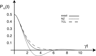
Figure 2: Time evolution of the population of the state $|{10}\rangle$ for a system initially prepared in the Bell state $\frac{1}{\sqrt{2}}\left(|{10}\rangle-|{01}\rangle\right)$. The width of the Lorentzian spectral density is $\lambda=\gamma$, the strength of the coupling constant between the two qubits is $\Omega=0.001\gamma$.

In fig.(2) the same quantity is reported choosing $\lambda=\gamma$. Despite the good agreement for the short time dynamics, we observe significant deviations when time increases. In particular concerning the long time behavior, the NZ equation leads to a very bad approximation. For times longer than some critical values the solution for the population $P_{10}(t)$ cannot represent a true diagonal element of a density matrix anymore, since it indeed assumes negative values. We may conclude that for this range of parameters the TCL solution gives a better description of the dynamics since it reproduces all the qualitative features of the exact solution.

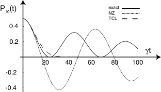
Figure 3: Time evolution of the population of the state $|{10}\rangle$ for a system initially prepared in the Bell state $\frac{1}{\sqrt{2}}\left(|{10}\rangle-|{01}\rangle\right)$. The width of the Lorentzian spectral density is $\lambda=0.01\gamma$, the strength of the coupling constant between the two qubits is $\Omega=0.001\gamma$.

Finally in fig.(3) we examine the regime $\lambda=0.01\gamma$ which, according to eq.(28), corresponds to very strong reservoir correlations and very long memory time. We observe once again a perfect agreement among all the three approaches in the short time behavior but in this case we assist at a failure of the TCL approach too. The solution of the TCL master equation (dashed line) doesn’t succeed to follow the Rabi’s oscillations witnessed by the exact dynamics (solid line). The NZ approaches presents the same problem of not conserving the positivity of the density matrix as in the previous case. Thus, in this case, both the perturbative approaches are not suitable to describe the dynamics of the system. It is interesting to observe that the oscillations appearing in the exact evolution of the populations $P_{10}(t)$ are not due to the spin-spin interaction constant $\Omega$, which we have taken small on purpose. The oscillations are instead due to the fact that, in this case, the Lorentzian peak is so narrow to make the environment equivalent to a cavity with losses, as one might verify for example by using the pseudomode approach in Refs.Mazzola ; garraway1 ; garraway2 ; garraway4 . Therefore, our exact solution in this regime, could be exploitable to describe the dynamics of two interacting qubits put inside two different optical cavities.

V Discussion and conclusive remarks

The problem of the proper description of open quantum systems is still far from having a complete and general solution. In particular, while the features of the Markovian dissipative dynamics are all well established and accepted, a lot of work has still to be done to claim general statements on the validity of the different possible non-Markovian approaches available in the literature.

In this paper we concentrated on the study of two popular methods aimed at describing non-Markovian dynamics: the Nakajima-Zwanzig and the time-convolutionless master equation approaches. Exploiting an exact solution for the dissipative dynamics of two coupled qubits interacting with independent reservoirs, we have shown that the TCL approach reproduces all the features of the non-Markovian dynamics for a range of parameters much wider than the one in which the NZ equation gives results which are physically reasonable, since the latter approach may violate the positivity condition on the density matrix already for reservoir correlations which are not very strong.

The discrimination of the best master equation approach for the problem under study is a very important issue, because the problem of the dissipative dynamics of two interacting qubits has been given a lot of attention in recent years, especially from the point of view of the entanglement dynamics quiroga ; sinaysky ; Tanas ; tanas 2008 ; grifoni ; storcz . So, once we have shown that for some parameters the TCL master equations provides a very good description of the non-Markovian dynamics, one may use the same approach for the description of temperature effects on the system dynamics, since we do not have at our disposal an exact solution of the dynamics at general reservoir temperatures.

We finally note that our exact solution can moreover be exploited in order to study the zero temperature entanglement dynamics in a range of parameters in which none of the two master equation approaches can be used: in this way one could extend the studies given in Refs. quiroga ; scala ; sinaysky , so that one could get the most general features of the quantum correlations between two qubits coupled to two independent reservoirs. These points will be the subject of our future research.

VI Acknowledgements

The authors acknowledge stimulating discussions with Prof. A. Messina. The authors also acknowledge partial support by MIUR Project N. II04C0E3F3. M.S. acknowledges financial support by the European Commission project EMALI.

References

- (1) A. Polyakov, Phys. Lett. 72B, 224 (1977).
- (2) A. Belitsky, V. Braun, A. Gorsky and G. Korchemsky, Int. J. Mod. Phys. A 19, 4715 (2004).
- (3) A. Baranco et al., Phys. Rev. Lett. 74, 4083 (1995).
- (4) L. Amico, R. Fazio, A. Ostorloh and V. Vedral, Rev.Mod. Phys. 80, 517 (2008).
- (5) R. McDermott, R. W. Simmonds, M. Steffen, K. B. Cooper, K. Cicak, K. D. Osborn, S. Oh, D. P. Pappas, and J. M. Martinis, Science 307, 1299 (2005).
- (6) J. B. Majer, F. G. Paauw, A. C. J. ter Haar, C. J. P. M. Harmans, and J. E. Mooij, Phys. Rev. Lett. 94, 090501 (2005).
- (7) T. Yamamoto, Y. A. Pashkin, O. Astafiev, Y. Nakamura, and J. Tsai, Nature 425, 941 (2003).
- (8) A. J. Berkley, H. Xu, R. C. Ramos, M. A. Gubrud, F. W. Strauch, P. R. Johnson, J. R. Anderson, A. J. Dragt, C. J. Lobb, and F. C. Wellstood, Science 300, 1548 (2003).
- (9) Y. A. Pashkin, T. Yamamoto, O. Astafiev, Y. Nakamura, D. Averin, and J. Tsai, Nature 421, 823 (2003).
- (10) B. Bellomo, R. Lo Franco, G. Compagno, Phys. Rev. Lett. 99, 160502 (2007).
- (11) B.M. Garraway, Phys. Rev. A 55, 2290 (1997).
- (12) B.M. Garraway, Phys. Rev. A 55, 4636 (1997).
- (13) B.J. Dalton, S.M. Barnett and B.M. Garraway, Phys. Rev. A 64, 053813 (2001).
- (14) Sumanta Das, G.S. Agarwal, arXiv:0905.3399 [quant-ph].
- (15) I. Sinaysky, F. Petruccione, D. Burgarth, Phys. Rev. A 78, 062301 (2008).
- (16) L. Quiroga, F.J. Rodríguez, M.E. Ramírez, R. París, Phys. Rev. A 75, 032308 (2007).
- (17) S. Maniscalco, F. Francica, R. L. Zaffino, N. Lo Gullo, F. Plastina, Phys. Rev. Lett. 100, 090503 (2008).
- (18) L. Mazzola, S. Maniscalco, J. Piilo, K.-A. Suominen, and B. M. Garraway, Phys. Rev. A 80, 012104 (2009)
- (19) T. Yu, J.H. Eberly, arXiv:0906.5378 [quant-ph].
- (20) M. Scala, R. Migliore, A. Messina, J. Phys. A: Math. Theor. 41, 435304 (2008).
- (21) S. Chaturvedi and F. Shibata, Z. Phys. B 35, 297 (1979).
- (22) S. Nakajima, Prog. Theor. Phys. 70, 948 (1958).
- (23) R. Zwanzig, J. Chem. Phys. 33, 1338 (1960).
- (24) B.L. Hu, J.P. Paz, Y. Zhang, Phys. Rev. D 45, 2843 (1992).
- (25) H.-P. Breuer and F. Petruccione, The Theory of Open Quantum Systems, Oxford University Press (2002).
- (26) I. Sinayskiy, E. Ferraro, A. Napoli, A. Messina, F. Petruccione, arXiv:0906.1796 [quant-ph].
- (27) R. W. Simmonds, K. M. Lang, D. A. Hite, S. Nam, D. P. Pappas, and John M. Martinis, Phys. Rev. Lett. 93, 077003 (2004).
- (28) R. Tanas, Z. Ficek, J. Opt. B Quantum Semiclass. Opt. 6, S90 (2004); Phys. Rev. A, 74, 024304 (2008).
- (29) R. Tanas, Z. Ficek, Phys. Rev. A, 77, 054301 (2008).
- (30) M. Governale, M. Grifoni and G. Schön, Chem. Phys. 268, 273 (2001).
- (31) M. J. Storcz, F. Hellmann, C. Hrelescu, and F. K. Wilhelm, Phys. Rev. A 72, 052314 (2005).