Stochastic dynamics and control of a driven nonlinear spin chain: the role of Arnold diffusion

Abstract

We study a chain of non-linear, interacting spins driven by a static and a time-dependent magnetic field. The aim is to identify the conditions for the locally and temporally controlled spin switching. Analytical and full numerical calculations show the possibility of stochastic control if the underlying semi-classical dynamics is chaotic. This is achievable by tuning the external field parameters according to the method described in this paper. We show analytically for a finite spin chain that Arnold diffusion is the underlying mechanism for the present stochastic control. Quantum mechanically we consider the regime where the classical dynamics is regular or chaotic. For the latter we utilize the random matrix theory. The efficiency and the stability of the non-equilibrium quantum spin-states are quantified by the time-dependence of the Bargmann angle related to the geometric phases of the states.

I Introduction

Advances in nanoscale fabrication of magnetic materials down to a finite chain of individual magnetic atoms science triggered a number of studies on the ground state magnetic properties of finite, interacting spin chains spintheory . For accessing the non-equilibrium states, in a linear chain one conventionally rotates the spins by applying a static magnetic field $\mathbf{H}_{0}$ and a variable magnetic field $\mathbf{h}(t)$ along a direction perpendicular to $H_{0}$ Abragam . The spins affected by the fields are then deflected by an angle $\theta=\omega_{1}\tau$ which can be desirably varied by changing the duration $\tau$ of the field $\mathbf{h}(t)$. Here $\omega_{1}$ is the amplitude of $\mathbf{h}(t)$ in frequency units $\omega_{1}=h_{0}\gamma$ ($\gamma$ is the gyromagnetic ratio). For this scheme to be viable $\omega_{1}$ has to be in resonance with the system precessional frequency. In this paper we consider the spin deflection in the different situation of a nonlinear chain of interacting spins Mejia-Monasterio ; Saito in which case the precessional frequency is dynamical and changes with the oscillation amplitude Sagdeev . Hence, a control strategy Matos-Abiague ; Matos-Abiague2 as in the linear chain case entails the use of chirped fields. Here we inspect a different route to spin control by exploiting the stochastic nature of the spin dynamics when appropriate fields are employed. This we show in a first step analytically. The advantage is that no special frequency tuning is used and more importantly the spin may be quasi stable at the deflected (non-equilibrium) angles when the field $\mathbf{h}(t)$ is off which might be of interest for quantum information applications Yuan ; Tuchette ; Mabuchi ; Hood ; Raimond ; Chotorlishvili ; Lakshmanan ; Zolotaryuk . Disadvantage is the limited control of the switching time. Full numerical simulations confirm our analytical predictions: Tuning the external fields such that the underlying classical spin dynamics is chaotic, stochastic switching occurs and a long-time quasi stabilization, i.e. a dynamical freezing (DF) of the deflected states is possible. Small fields cause only small fluctuations around the equilibrium state. For very strong fields, effects of magnetic anisotropy and exchange become subsidiary and hence the dynamics turn regular and no deflection with subsequent freezing is possible.

For a finite spin chain we uncover analytically that our stochastic control (SC) scheme is governed by Arnold diffusion and give analytical expression for the Arnold diffusion coefficient that in turn determine the time scale for SC.

To inspect the influence of the quantum nature of the spins on our (classical) predictions we considered both the regular and the chaotic classical regimes and evaluated the so-called Bargmann angle which is a measure of the quantum distance between states in the Hilbert space and can be used to signal DF Matos-Abiague ; Matos-Abiague2 . Using random matrix theory we prove indeed that SC and DF are possible at the driving field values that follows from our classical analysis.

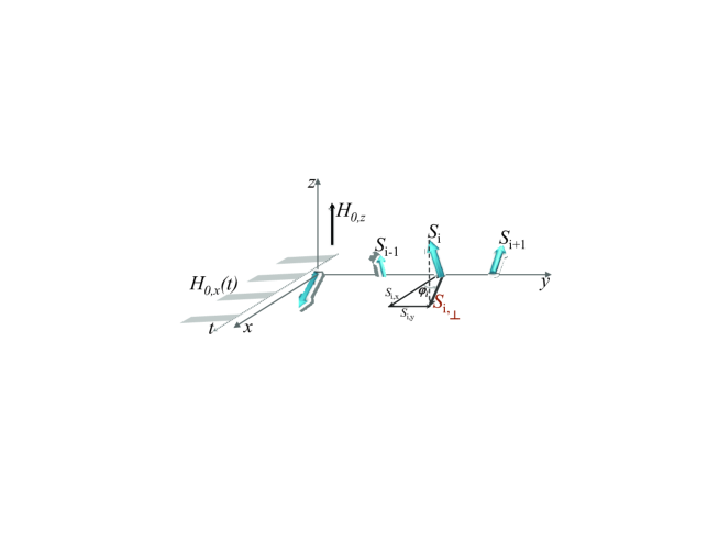
Figure 1: A schematics of the interacting spin chain. The magnetic anisotropy field sets the $z$ direciton. Two magnetic fields are applied: a static ($H_{0,z}$) one along the $z$ axis and a time-dependent field ($H_{0,x}(t)$) along the $x$ axis.

II Equation of motion

II.1 Liouville equation for the spin chain

Similar to the case studied in Mejia-Monasterio ; Saito we consider a system that can be modeled by a chain of $N$ interacting (with coupling constant $J$) spin variables localized at sites $j$ and having a uniaxial anisotropy with the anisotropy constant $\beta$. Possible sources of the anisotropy field are discussed in Refs.science . Here we mention that the inclusion of a finite anisotropy is essential for the existence of a finite-temperature long-range order in the (infinitely long) chain. Further important consequences of the magnetic anisotropy for the phenomena discussed in this work are detailed below. The direction of the anisotropy field defines the $z$ axis. A static ($H_{0z}$) and a time-dependent ($H_{0x}(t)$) magnetic fields are applied along the $z$ and $x$ axes, respectively (cf. Fig.1). $H_{0x}(t)$ consists of $N_{k}$ periodic pulses, i.e.

$$H_{0x}(t)=\varepsilon T\sum\limits_{k}^{N_{k}}\delta(t-kT),$$ (1)

where $T$ is the period and $\varepsilon T$ is the field strength. As demonstrated explicitly prl09 (for the classical spin dynamics) the shape (1) of the field mimics well the action of a finite-width pulse as long as the pulse duration is smaller than the field-free precessional period of the spins. The time-integral over the field amplitude of the finite-width pulse sets the variables $\varepsilon$ prl09 .

From the Hamilton operator Mejia-Monasterio ; Saito

$$\hat{H}=\sum\limits_{j=1}^{N-1}J\hat{s}_{jz}\hat{s}_{j+1,z}+H_{0x}\sum\limits_{j=1}^{N}\hat{s}_{jx}+H_{0z}\sum\limits_{j=1}^{N}\hat{s}_{jz}+\beta\sum\limits_{j=1}^{N}\hat{s}^{2}_{jz}$$ (2)

we find the spin equation of motion (EOM) to be

$$\partial_{t}\mathbf{\hat{s}}_{j}=\mathbf{h}_{j}\times\mathbf{\hat{s}}_{j},\quad\mathbf{h}_{j}=\left(H_{0x},0,J[{\hat{s}}_{j+1z}+{\hat{s}}_{j-1z}]+H_{0z}+2\beta\hat{s}_{jz}\right).$$ (3)

For large spins $s_{j}$ with $\hbar s_{j}(s_{j}+1)=\langle\mathbf{{\hat{s}}}_{j}\rangle$ and $[\hat{H},\mathbf{\hat{s}}_{i}^{2}]=0$ we shift variables as (cf. Fig.1, $s_{i}^{2}=1$)

$$s_{ix}=s_{i\perp}\cos\varphi_{i};~{}~{}~{}s_{iy}=s_{i\perp}\sin\varphi_{i},\ s_{i,\perp}=\sqrt{1-s_{i,z}^{2}}.$$ (4)

EOM for two spins $N=2$ in term of the canonical action variables $s_{1z},$ $s_{2z}$ and their conjugate angles $\varphi_{1},$ $\varphi_{2}$ reads

$$\dot{s}_{iz} = -\varepsilon\frac{\partial V}{\partial\varphi_{i}},\quad\dot{\varphi}_{i}=\omega_{i}(s_{jz})+\varepsilon\frac{\partial V}{\partial s_{iz}},\quad\omega_{i}(s_{jz})=Js_{jz}+2\beta\hat{s}_{iz}+H_{0z},\quad i,j\in\{1,2\};$$

$$V := \sum\limits_{i=1}^{N}V_{i}(s_{iz},\varphi_{i})=\sum\limits_{i=1}^{N}V_{0i}(s_{iz},\varphi_{i})\ T\sum\limits_{k=-\infty}^{+\infty}\delta(t-kT)=\sum\limits_{i=1}^{N}s_{i\perp}\cos\varphi_{i}\cdot T\sum\limits_{k=-\infty}^{+\infty}\delta(t-kT).$$

For $V\neq 0$ the variables of actions are adiabatic invariants and hence are slow with respect to the angles typical time scale Sagdeev . The idea now is to identify the regime of classical chaotic dynamics which we will do below. In this regime one may adopt a kinetic approach based on the Liouville equation Balescu ; Lichtenberg for the two-particle distribution function $f(t,s_{1z},\varphi_{1},s_{2z},\varphi_{2})$, i.e.

$$i\frac{\partial f}{\partial t} = \big{(}\hat{L}_{0}+\varepsilon\hat{L}_{1}\big{)}f,$$

$$\hat{L}_{0} = -i\omega_{1}(s_{2z})\frac{\partial}{\partial\varphi_{1}}-i\omega_{2}(s_{1z})\frac{\partial}{\partial\varphi_{2}},$$

$$\hat{L}_{1} = -i\Bigg{(}\frac{\partial V}{\partial s_{1z}}\,\frac{\partial}{\partial\varphi_{1}}-\frac{\partial V}{\partial\varphi_{1}}\,\frac{\partial}{\partial s_{1z}}\Bigg{)}-i\Bigg{(}\frac{\partial V}{\partial s_{2z}}\,\frac{\partial}{\partial\varphi_{2}}-\frac{\partial V}{\partial\varphi_{2}}\,\frac{\partial}{\partial s_{2z}}\Bigg{)}.$$ (6)

Eq.(6) is of a key importance for this study. Below we use the random phase approximation and some mathematical techniques to derive from eg.(6) the Fokker-Planck equation which allows to explore some chaotic features of the spin dynamics.

II.2 Fokker-Planck formulation and the onset of the chaotic regime

Expressing $f(s_{1z},\varphi_{1},s_{2z},\varphi_{2})$ as a Fourier series over $\varphi_{1}$ and $\varphi_{2}$ we find

$$f(s_{1z},\varphi_{1},s_{2z},\varphi_{2}) = \frac{1}{(2\pi)^{2}}\sum_{m,n}\bar{f}_{n,m}(s_{1z},s_{2z})e^{in\varphi_{1}}e^{im\varphi_{2}},$$

$$\bar{f}_{n,m}(s_{1z},s_{2z}) = f_{n,m}(s_{1z},s_{2z})\cdot\exp\big{[}-in\int\limits_{0}^{t}\omega_{1}(t^{\prime})dt^{\prime}\big{]}\cdot\exp\big{[}-im\int\limits_{0}^{t}\omega_{2}(t^{\prime})dt^{\prime}\big{]},$$

$$\omega_{1}\big{(}t^{\prime}\big{)} = \omega_{1}\big{(}s_{2z}(t^{\prime})\big{)},\omega_{2}\big{(}t^{\prime}\big{)}=\omega_{2}\big{(}s_{1z}(t^{\prime})\big{)}.$$ (7)

Hence, solution of the Liouville equation is cast formally as (the symbol $\langle n^{\prime},m^{\prime}|\hat{L}_{1}(t_{1})|n,m\rangle$ means the average over fast oscillating variables)

$$f_{n^{\prime},m^{\prime}}\big{(}s_{1z},s_{2z},t\big{)}=f_{n^{\prime},m^{\prime}}\big{(}s_{1z},s_{2z},0\big{)}-$$

$$-i\varepsilon\sum_{n,m}\int\limits_{0}^{t}dt_{1}e^{i(n^{\prime}-n)\int\limits_{0}^{t_{1}}\omega_{1}(t^{\prime})dt^{\prime}}e^{i(m^{\prime}-m)\int\limits_{0}^{t_{1}}\omega_{2}(t^{\prime})dt^{\prime}}\langle n^{\prime}m^{\prime}|\hat{L}_{1}(t_{1})|n,m\rangle f_{n,m}\big{(}s_{1z},s_{2z},t_{1}\big{)}.$$ (8)

If the interaction energy with the variable field is small with respect to the other terms in eq.(2) we can expand $f$ in terms of the field strength $\varepsilon$ and account for leading terms only.

The zero-order component has the form

$$f_{0,0}\big{(}s_{1z},s_{2z},t\big{)}=f_{0,0}\big{(}s_{1z},s_{2z},0\big{)}-$$

$$-i\varepsilon\sum_{n,m}\int\limits_{0}^{t}dt_{1}e^{-in\int\limits_{0}^{t_{1}}\omega_{1}(t^{\prime})dt^{\prime}}e^{-im\int\limits_{0}^{t_{1}}\omega_{2}(t^{\prime})dt^{\prime}}\langle 0,0|\hat{L}_{1}(t_{1})|n,m\rangle f_{n,m}\big{(}s_{1z},s_{2z},0\big{)}+$$ (9)

$$+(-i\varepsilon)^{2}\sum_{n,m}\int\limits_{0}^{t}dt_{1}\int\limits_{0}^{t_{1}}dt_{2}e^{in\int\limits_{t_{1}}^{t_{2}}\omega_{1}(t^{\prime})dt^{\prime}}e^{im\int\limits_{t_{1}}^{t_{2}}\omega_{2}(t^{\prime})dt^{\prime}}\langle 0,0|\hat{L}_{1}(t_{1})|n,m\rangle\langle n,m|\hat{L}_{1}(t_{2})|0,0\rangle f_{0,0}\big{(}s_{1z},s_{2z},0\big{)}.$$

Now we write $\hat{L}_{1}$ as a Fourier series taking the relevant frequency $\Omega=\frac{2\pi}{T}$ into account, $\hat{L}_{1}(t)=\sum_{p}L_{1,p}\exp(ip\Omega t),L_{1,-p}=L_{1,p}^{\ast}$. Inserting into (9) we find

$$f_{0,0}\big{(}s_{1z},s_{2z},t\big{)}=f_{0,0}\big{(}s_{1z},s_{2z},0\big{)}-$$

$$-i\varepsilon\sum_{n,m}\int\limits_{0}^{t}dt_{1}e^{-in\int\limits_{0}^{t_{1}}\omega_{1}(t^{\prime})dt^{\prime}}e^{-im\int\limits_{0}^{t_{1}}\omega_{2}(t^{\prime})dt^{\prime}}\langle 0,0|\hat{L}_{1}(t_{1})|n,m\rangle f_{n,m}\big{(}s_{1z},s_{2z},0\big{)}+$$ (10)

$$+(-i\varepsilon)^{2}\sum_{n,m,p}\int\limits_{0}^{t}dt_{1}\int\limits_{0}^{t_{1}}dt_{2}e^{in\int\limits_{t_{1}}^{t_{2}}\omega_{1}(t^{\prime})dt^{\prime}}e^{im\int\limits_{t_{1}}^{t_{2}}\omega_{2}(t^{\prime})dt^{\prime}}\langle 0,0|\hat{L}_{1,p}(t_{1})|n,m\rangle\langle n,m|\hat{L}_{1,-p}(t_{2})|0,0\rangle\,$$

$$e^{ip\Omega(t_{1}-t_{2})}f_{0,0}\big{(}s_{1z},s_{2z},0\big{)}.$$

Introducing the notations

$$\psi_{1}(t_{1},t_{2})=\int\limits_{t_{1}}^{t_{2}}\omega_{1}(t^{\prime})dt^{\prime},\;\psi_{2}(t_{1},t_{2})=\int\limits_{t_{1}}^{t_{2}}\omega_{2}(t^{\prime})dt^{\prime}$$ (11)

we write

$$f_{0,0}\big{(}s_{1z},s_{2z},t\big{)}=f_{0,0}\big{(}s_{1z},s_{2z},0\big{)}-$$

$$-i\varepsilon\sum_{n,m}\int\limits_{0}^{t}dt_{1}e^{-in\psi_{1}(t_{1},0)}e^{-im\psi_{2}(t_{1},0)}\langle 0,0|\hat{L}_{1}(t_{1})|n,m\rangle f_{n,m}\big{(}s_{1z},s_{2z},0\big{)}+$$ (12)

$$+(-i\varepsilon)^{2}\sum_{n,m,p}\int\limits_{0}^{t}dt_{1}\int\limits_{0}^{t_{1}}dt_{2}e^{-in\psi_{1}(t_{1},t_{2})}e^{-im\psi_{2}(t_{1},t_{2})}\langle 0,0|\hat{L}_{1,p}|n,m\rangle\langle n,m|\hat{L}_{1,-p}|0,0\rangle\cdot$$

$$\cdot e^{ip\Omega(t_{1}-t_{2})}f_{0,0}\big{(}s_{1z},s_{2z},0\big{)}.$$

Averaging over the initial phases, i.e. $F\big{(}s_{1z},s_{2z},t\big{)}=\Bigg{\langle}\Big{\langle}f_{0,0}\big{(}s_{1z},s_{2z},t\big{)}\Big{\rangle}\Bigg{\rangle}$, and using the random phase approximation $\psi_{1}(t_{1},t_{2})=\int\limits_{t_{1}}^{t_{2}}\omega_{1}(t^{\prime})dt^{\prime}\approx\varphi_{1}(t_{2})-\varphi_{1}(t_{2}),$ we end up with

$$\Bigg{\langle}\Big{\langle}\exp\big{[}in\psi_{1,2}(t_{2},t_{1})\big{]}\Big{\rangle}\Bigg{\rangle}=\exp\big{(}-(t_{1}-t_{2})/\tau_{c}\big{)}\exp\big{(}-in\omega_{1,2}(t_{1}-t_{2})\big{)}.$$ (13)

Here $\tau_{c}$ is the correlation time of random phase. Taking eq.(12) into account we deduce then for the averaged two-particle distribution function $F(t)$ the dynamical equation (up to a second order in the field strength $\varepsilon$)

$$\frac{\partial F}{\partial t}=-i\varepsilon e^{-\frac{2t}{\tau_{c}}}\sum\limits_{n,m}e^{-i(n\omega_{1}+m\omega_{2})t}\langle 0,0|\hat{L}_{1}(t)|n,m\rangle f_{n,m}(s_{1z},s_{2z},0)-$$

$$-\varepsilon^{2}\frac{\partial}{\partial t}\sum\limits_{m,n,p}\int\limits_{0}^{t}dt_{1}\int\limits_{0}^{t_{1}}dt_{2}e^{-\frac{2(t_{1}-t_{2})}{\tau_{c}}}e^{-in\omega_{1}(t_{1}-t_{2})}e^{-im\omega_{2}(t_{1}-t_{2})}e^{ip\Omega(t_{1}-t_{2})}$$ (14)

$$\langle 0,0|L_{1,p}|n,m\rangle\langle m,n|L_{1,-p}|0,0\rangle F(s_{1z},s_{2z},t).$$

The long time behaviour ($t\gg\tau_{c}$) is retrieved by shifting to the new variables $\tau=t_{1}-t_{2}$,$t_{1}=t_{1}$ in (14) and integrating over $\tau$ which yields

$$\frac{\partial F}{\partial t}=-\varepsilon^{2}\sum\limits_{n,m,p}\frac{1}{\frac{2}{\tau_{c}}+i(n\omega_{1}+m\omega_{2}-p\Omega)}\langle 0,0|L_{1p}|n,m\rangle\langle m,n|L_{1,-p}|0,0\rangle F(s_{1z},s_{2z},t).$$ (15)

For a further progress explicit expressions for the matrix elements $\langle 0,0|L_{1,p}|n,m\rangle\langle m,n|L_{1,-p}|0,0\rangle$ are need. Following the standard procedure outlined in Haken we find after some lengthy steps the following Fokker-Planck equation for $F(s_{1z},s_{2z},t)$

$$\frac{\partial F(s_{1z},s_{2z},t)}{\partial t}=D\Bigg{(}\frac{\partial}{\partial s_{1z}}(1-s_{1z}^{2})\frac{\partial F}{\partial s_{1z}}+\frac{\partial}{\partial s_{2z}}(1-s_{2z}^{2})\frac{\partial F}{\partial s_{2z}}\Bigg{)},\quad D=\frac{\varepsilon^{2}\pi}{2\Omega}=\frac{\varepsilon^{2}T}{4}.$$ (16)

Making the ansatz $F(s_{1z},s_{2z})=F_{1}(s_{1z})F_{2}(s_{2z})$ the average values of the spin projections $\bar{s}_{jz}$ is determined from

$$\frac{d}{dt}\bar{s}_{jz} = \int\limits_{-1}^{+1}s_{jz}\frac{\partial F_{j}}{\partial t}ds_{jz}=D\int\limits_{-1}^{+1}s_{1z}\frac{\partial}{\partial s_{jz}}(1-s_{jz}^{2})\frac{\partial F_{j}(s_{jz})}{\partial s_{jz}}=-2D\bar{s}_{jz};\>j=1,2;$$

$$\bar{s}_{1,2z} = s_{1,2z}(0)e^{-2Dt}.$$ (17)

As discussed in levanpla (for the case without anisotropy field), essential for the validity of this diffusion type dynamics is that the underlying classical dynamics is chaotic in which case the above derivations are justified.

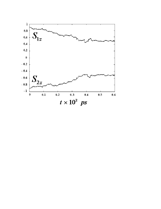
Figure 2: The time evolution of $s_{1z}$ and $s_{2z}$ for the following parameters of the system: $J=0.2$,  $2\beta=0,1$,  $H_{0z}=0.2$,  $\varepsilon=0.057$,  $\Omega=100$.  $\frac{\tau_{0}}{T}=0.1$,  $s_{1z}(0)=0.8$,   $\varphi_{1}(0)=0$,  $s_{2z}(0)=-0.8$,  $\varphi_{2}(0)=0$,  $T=\frac{2\pi}{\Omega}$ and $K_{0}=K^{\prime}=0.45\cdot 10^{-4}$.

The stroboscopic evolution of the spin variables before ($t_{0}-\tau$) and after ($t_{0}+\tau$) applying the field pulses at $t=t_{0}$ is expressed as levanpla

$$s_{iz,n+1} = s_{iz,n}+\varepsilon T\sqrt{1-s_{iz,n}^{2}}\sin\varphi_{i,n},$$

$$\varphi_{i,n+1} = \varphi_{i,n}+\bigg{(}Js_{jz,n+1}+2\beta s_{iz}-H_{0z}\bigg{)}T-\varepsilon T\frac{s_{iz,n}}{\sqrt{1-s_{iz,n}^{2}}}\cos\varphi_{i,n}.$$ (18)

The stability of the trajectories is deduced from the Jacobian matrix Chirikov which also set the condition for the chaotic regime as ($<...>_{t}$ means time average)

$$|\lambda_{i}|>1, K>0,$$ (19)

$$\lambda_{1,2} = \frac{(2+K)\pm\sqrt{(K+2)^{2}-4}}{2},~{}~{}~{}\lambda_{3,4}=\frac{(2-K)\pm\sqrt{(K-2)^{2}-4}}{2},$$

$$K = K_{0}\sqrt{(\beta/J)^{2}+(1-2(\beta/J)^{2})s_{1\perp}s_{2\perp}<\cos\varphi_{1}\cos\varphi_{2}>_{t}},~{}~{}~{}K_{0}=\varepsilon T^{2}J.$$ (20)

Hence we can tune to the chaotic regime by varying the external fields parameters, the constant of anisotropy $\beta$, and the coupling constant $J$ between adjacent spins. For evaluating averages of the form $<...>_{t}$ averages over time correlation functions of the random phases $<\cos\varphi_{1}\cos\varphi_{2}>$ should be considered. For the correlation term we proceed as follows: When deriving the diffusion equation we assumed that correlation time of random phases are small with respect to the diffusion scale $\tau_{c}<<\frac{2D}{\pi\varepsilon}=1/\Omega$. Taking into account that in this time scale values $s_{1,2\bot}$ are slow in time, after averaging of correlation functions over the time interval $\Delta t\in\left(0,1/\Omega\right)$ we obtain $K=K_{0}\sqrt{(\beta/J)^{2}+(1-2(\beta/J)^{2})\frac{\varepsilon\pi}{2D}s_{1\perp}s_{2\perp}\tau_{c}(J)}.$

II.3 Discussions and numerical results

Having discussed the analytical structure of the spin dynamics we compare the analytical predictions with full numerical simulations of the problem.

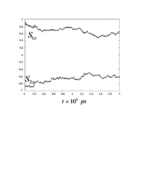
Figure 3: Same quantities as in Fig.(2) however, $J=0.2$, $2\beta=0.1$, $H_{0z}=0.2$,  $\varepsilon=0.04$,  $\Omega=100$.  $\frac{\tau_{0}}{T}=0.1$,  $s_{1z}(0)=0.9$,   $\varphi_{1}(0)=0$,  $s_{2z}(0)=-0.9$,  $\varphi_{2}(0)=0$,   $T=\frac{2\pi}{\Omega}$ and $K_{0}=0.32\cdot 10^{-4}<K^{\prime}$.

Note, our system is such that the conditions of chaotic regime eq.(19),(20) can be realized for arbitrary small perturbation $\varepsilon>0,~{}~{}K_{0}>0$. However, the smallest values of $\varepsilon$, and corresponding $K_{0}=K^{{}^{\prime}}$ that allows for an observable effect has to be found numerically. At first, the external fields are tuned to $K_{0}=K^{\prime}=0.45\cdot 10^{-4}>0$. In accord with the analytical results stochastic switching of the initial spins direction occur accompanied with a subsequent long-time stabilization (see Fig.(2)). If the fields are such that $K_{0}<K^{\prime}$ (i.e. $K_{0}$ is very small) switching does not happen (see Fig.(3)), i.e. $s_{1,2z}$ is still an adiabatic invariants; external fields lead to small fluctuations around the equilibrium state. We note that in Fig.(3) the anisotropy field is finite but its effect is hardly observable becomes of it smallness $\left({\beta/J}\right)^{2}=0.06$. The regular (but non-integrable) regime is reached by applying very strong fields ($\varepsilon T\gg J$, $H_{oz}\gg Js^{z}>2\beta s^{z}$) (cf. eq. (3)). In this case no stochastic switching occurs (cf. Fig.4.). The eigenfrequency of the system is given by the constant magnetic field $\omega_{j}(S_{iz})=JS_{iz}+H_{0z}+2\beta s_{jz}\approx H_{0z}$. Physically, effects related to the exchange interaction and to the anisotropy field become negligible and we end up with the familiar resonant switching scheme (this is true only during the time when the external fields are on. Effects of exchange and anisotropy govern the subsequent field-free dynamics. A scheme for a field-induced deflection and freezing has been proposed in Ref.[prl09, ]).

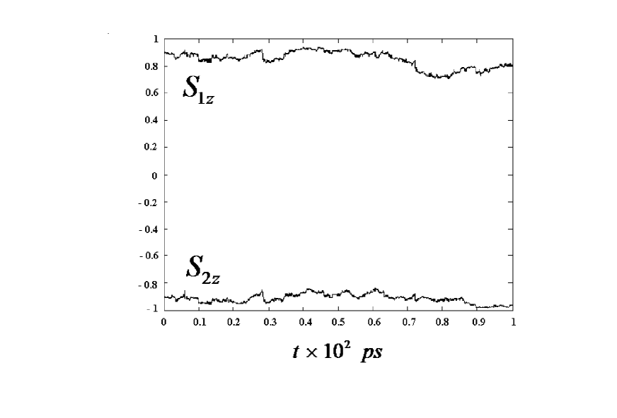
Figure 4: Same quantities as in Fig.3 however, $J=0$,  $\beta=0$,  $H_{0z}=0.2$,  $\varepsilon=0.04$,  $\Omega=100$.  $\frac{\tau_{0}}{T}=0.1$,  $s_{1z}(0)=0.9$,   $\varphi_{1}(0)=0$,   $s_{2z}(0)=-0.9$,  $\varphi_{2}(0)=0$,  $T=\frac{2\pi}{\Omega}$ and $K_{0}=0$.

II.4 Finite spin chain

The EOM for a finite spin chain governing the dynamics of each particular spin follows from (2) as

$$\frac{ds_{iz}}{dt}=-\varepsilon\frac{\partial V_{i}\left(\varphi_{i},s_{iz}\right)}{\partial\varphi_{i}},~{}~{}~{}~{}~{}~{}~{}~{}~{}~{}~{}~{}~{}~{}~{}~{}~{}~{}~{}~{}$$

$$\frac{d\varphi_{i}}{dt}=\omega_{i}\left(s_{i-1z},s_{iz},s_{i+1z}\right)+\varepsilon\frac{\partial V_{i}\left(\varphi_{i},s_{iz}\right)}{\partial s_{iz}},$$ (21)

$$\omega_{i}\left(s_{i-1z},s_{iz},s_{i+1z}\right)=Js_{i-1z}+Js_{i+1z}+2\beta s_{iz}+H_{0z},~{}~{}~{}i=1,..N.~{}~{}~{}~{}N+1=N.~{}~{}~{}~{}~{}~{}~{}~{}~{}~{}~{}~{}~{}$$

If the variable field has a spatial extent such that only two spins in the chain, labeled $(k,k+1)$, are affected then we find

$$\frac{ds_{iz}}{dt}=-\left(\delta_{i,k}+\delta_{i,k+1}\right)\varepsilon\frac{\partial V_{i}\left(\varphi_{i},s_{iz}\right)}{\partial\varphi_{i}},~{}~{}~{}~{}~{}~{}~{}~{}~{}~{}~{}~{}$$

$$\frac{d\varphi_{i}}{dt} = \omega_{i}\left(s_{i-1z},s_{iz},s_{i+1z}\right)+\left(\delta_{i,k}+\delta_{i,k+1}\right)\varepsilon\frac{\partial V_{i}\left(\varphi_{i},s_{iz}\right)}{\partial s_{iz}},$$

$$s_{iz}(t) = constant\quad\mbox{if}\quad k\neq i\neq k+1.$$ (22)

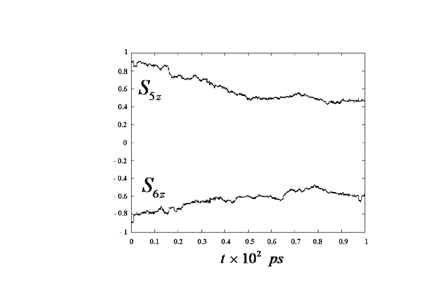
Figure 5: We consider a chain of 10 interacting spins. We show here the dynamics of the $z$ components $s_{5,z}$ and $s_{6,z}$ of the spins labelled $5$ and $6$. Other parameters are $J=0.2$,    $2\beta=0,3$,   $H_{0z}=0.2$,  $\varepsilon=0.04$,  $\Omega=100$.  $\frac{\tau_{0}}{T}=0.1$,  $s_{2n+1}^{z}(0)=0.9$,   $s_{2n}^{z}(0)=0.9$,  $\varphi_{i}(0)=0$,  $T=\frac{2\pi}{\Omega}$,  $i=\overline{1,N}$.    $N=10$.

These equations show that the $z$ component of the spins subjected to the pulse have to be determined self-consistently. The dynamics of the oscillation frequency of the spins transverse components $\dot{\varphi}_{i},~{}~{}i=1...N$ is determined by the effective magnetic field as

$$\dot{\varphi}_{i}(t)=\omega_{i}^{eff}=\gamma_{s}H_{i}^{eff}(t).$$ (23)

Here

$$H^{eff}(t)=\frac{1}{\gamma_{s}}\bigg{[}H_{0}+J(S_{i-1,z}+S_{i+1,z})+\bigg{(}2\beta-(\delta_{i,k}+\delta_{i,k+1})\frac{H_{0x}(t)}{S_{i\bot}}\textrm{cos}(\varphi_{i})\bigg{)}S_{i,z}\bigg{]}.$$

This indicates that the spins subject to the pulses exchange energy with their nearest neighbors (whose $z$ components are nevertheless constant). This process depends on the values of the $z$ components and on the effective frequency $\omega_{i}^{eff}(t)s_{i}^{z}(t)$; a demonstration of this phenomena is shown in Fig.5.

A further tool for controlling the diffusion process is to apply a constant field along the $x$ axis. The system dynamics is then chaotic, even without the periodic series of pulses Mejia-Monasterio ; Saito . Therefore, the $z$ component of the spin is not an adiabatic invariant and the mechanism of dynamical freezing (DF) discussed above does not work. Fig.6 illustrates that if the amplitude of the magnetic field applied along $x$ axis is strong enough $H_{0x}>H_{0z}$ then the longitudinal component of the spin performs fast oscillations. In the other opposite case $H_{0x}<H_{0z}$ the orientation of the spin can be deflected but DF again is not possible (cf. Fig 7).

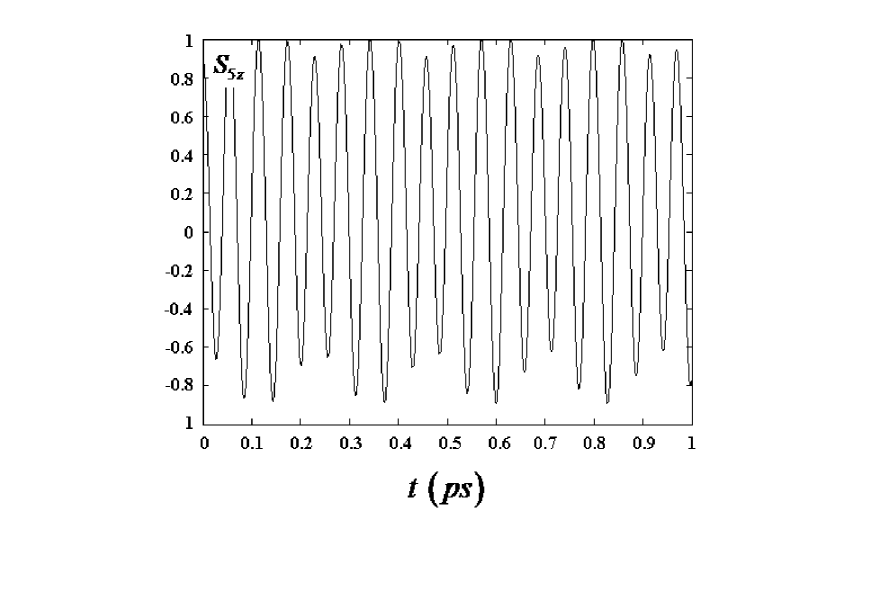
Figure 6: The time dependence of the $z$ component of $5^{rmth}$ spin for the parameters $J=0.2$,  $H_{0z}=0.2$,  $\beta=0$  $H_{0x}=1$,  $s_{2n+1}^{z}(0)=0.9$,   $s_{2n}^{z}(0)=-0.9$,  $\varphi_{i}(0)=0$,  $i=\overline{1,N}$,  $N=10$.

Figure 7: The same as in Fig. 6 however the parameters are changed to $J=0.2$,  $H_{0z}=0.2$,  $H_{0x}=0.01$,   $s_{2n+1}^{z}(0)=0.9$,  $s_{2n}^{z}(0)=-0.9$,  $\varphi_{i}(0)=0$,   $i=\overline{1,N}$,  $N=10$.

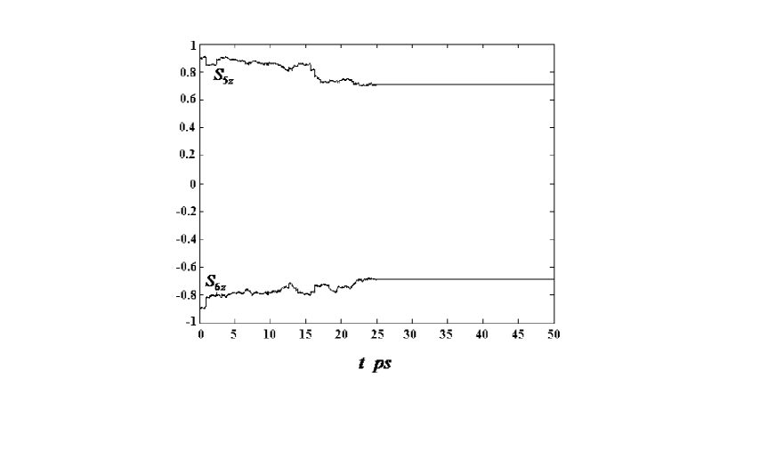
Figure 8: The $z$ components of the spins labelled $5$ and $6$ for the parameters: $J=0.2$,  $H_{0z}=0.2$,  $H_{0x}=0.01$,  $s_{2n+1}^{z}(0)=0.9$,   $s_{2n}^{z}(0)=-0.9$,  $\varphi_{i}(0)=0$,  $i=\overline{1,N}$,  $N=10$.

After deflection of the spin to a desired angle, one can completely freeze its orientation. Key point is the fact that, in the absence of pulses the $z$ component of the spin projection is an integral of motion. The system of equations in this case has the form

$$\frac{ds_{jx}}{dt}=-J\big{(}s_{j-1,z}+s_{j+1,z}\big{)}s_{jy}-H_{0z}s_{jy},$$

$$\frac{ds_{jy}}{dt}=J\big{(}s_{j-1,z}+s_{j+1,z}\big{)}s_{jx}+H_{0z}s_{jx},$$ (24)

$$\frac{ds_{jz}}{dt}=0.$$

For simplicity we assumed here that $\beta=0$. After solving(24) one obtains

$$s_{jx}=s_{jx}\big{(}t_{0}\big{)}\cos\big{(}\omega_{j0}t+\varphi_{0}\big{)},$$

$$s_{jy}=s_{jy}\big{(}t_{0}\big{)}\sin\big{(}\omega_{j0}t+\varphi_{0}\big{)},$$ (25)

$$s_{jz}=s_{jz}\big{(}t_{0}\big{)},$$

where $\omega_{j}\bigg{(}s_{j-1z}\big{(}0\big{)};s_{j+1z}\big{(}0\big{)}\bigg{)}=J\bigg{(}s_{j-1z}\big{(}0\big{)}+s_{j+1z}\big{(}0\big{)}\bigg{)}+H_{0z}=\omega_{j0}$, and $s_{jz}\big{(}t_{0}\big{)}$ corresponds to the desired orientation of the spin, achieved after the action of the pulses in the time interval $0<t<t_{0}$ (cf Fig.8).

II.5 Arnold Diffusion

Results of previous section evidence that even in the case of a long spin chain the orientation of spins can be still controlled. This follows from resonance overlapping and the existence of diffusion. However, the question of what kind of diffusion we have is still outstanding. If the dimension of the system is more than $N>2$, the dynamics is much more involved and the emergence of new physical phenomenon is expected. We recall the key idea of KAM theory: The size of the destroyed torus is small and the domain of their location is surrounded by invariant torus. This situation changes if an invariant torus crosses the domain of the destroyed torus location. This is possible if and only if $N>2$. The phenomenon of universal diffusion along the net formed due to the inter-tours crossing was discovered by Arnold Sagdeev . Here we consider the mechanism of the formation of the stochastic net in the case of a spin chain.

$$H=H_{0}(s^{z}_{1},...s^{z}_{N})+\varepsilon V(\varphi_{1},.....\varphi_{N}).$$ (26)

Note, the frequencies of the unperturbed motion on the $N$ dimensional torus is a function of the three actions

$$\omega_{i}(s^{z}_{i-1},s^{z}_{i},s^{z}_{i+1})=Js^{z}_{i-1}+Js^{z}_{i+1}+2\beta s^{z}_{i}+H_{0z},~{}~{}~{}~{}~{}i=\overline{1,N}.$$ (27)

We collect the resonant tours defined by the condition:

$$\sum\limits_{j=1}^{N}n_{j}\omega_{j}=0,$$ (28)

where $n_{j}$ are integer numbers. For each set of numbers there exists a multitude of solutions $s^{0}_{z}\equiv(s^{z(0)}_{1},...s^{z(0)}_{N})$. Each solution determines resonant tours. For the formation of the Arnold diffusion the absences of degeneracy is essential

$$det\bigg{|}\frac{\partial^{2}H_{0}}{\partial s^{z}_{i}\partial s^{z}_{j}}\bigg{|}\neq 0,~{}~{}~{}~{}i,j=\overline{1,N}.$$ (29)

In the case of our system due to the form of the matrix

$$\frac{\partial^{2}H_{0}}{\partial s^{z}_{i}\partial s^{z}_{j}}=\left(\begin{array}[]{c}2\beta~{}~{}J~{}~{}0~{}~{}0~{}~{}.\\ J~{}~{}2\beta~{}~{}J~{}~{}0~{}~{}.\\ 0~{}~{}J~{}~{}2\beta~{}~{}J~{}~{}.\\ 0~{}~{}0~{}~{}J~{}~{}2\beta~{}~{}.\\ .~{}~{}.~{}~{}.~{}~{}.~{}~{}.\end{array}\right),$$ (30)

the condition of the absence of a degeneration (29) leads to the polynomial expression

$$det\bigg{|}\frac{\partial^{2}H_{0}}{\partial s^{z}_{i}\partial s^{z}_{j}}\bigg{|}=G(J,\beta,N)\neq 0.$$ (31)

The explicit form of the expression (31) also depends on the system’s size (in addition to the dependence on the parameters $\beta,J$). For large systems we obtain the following asymptotic expressions

$$G(J,\beta,N)=J^{N}~{}~{}if~{}~{}J>\beta,~{}~{}~{}~{}G(J,\beta,N)=2^{N}\beta^{N}~{}~{}if~{}~{}J<\beta.$$ (32)

From this relation we can conclude that the universal diffusion is possible for any nonzero $J,\beta$, and identify the numeric results obtained for the spin chain with the Arnold diffusion. For an analytical estimation we consider the minimal possible dimension. Therefore, in what follows, without loss of generality we shall restrict ourselves by the case $N=3$. From eq.(28) we find

$$n_{1}\omega_{1}+n_{2}\omega_{2}+n_{3}\omega_{3}=0,$$ (33)

where each frequency depends on the three action according to (27). In the frequency space $(\omega_{1},\omega_{2},\omega_{3})$ eq. (33) determines a family of surfaces. On the energy surface we have

$$H_{0}(s^{z}_{1},s^{z}_{2},s^{z}_{3})=E.$$ (34)

This equation is also the equation determining the surface (33). Therefore, the resonant tours have a common parts along the curves, defined as the solutions of the set of equations (33), (34). The time dependent perturbation leads to a widening of these curves and to the formation of the stochastic net.

In order to provide topological interpretation of this phenomenon we will consider simplest case of three spins. In this case the explicit form of Eq (33) and Eq (34) reads:

$$(J+2\beta)(\omega_{1}^{2}+\omega_{2}^{2}+\omega_{3}^{2})-2\omega_{1}\omega_{2}-2\omega_{1}\omega_{3}-2\omega_{2}\omega_{3}=E,$$ (35)

and

$$n_{1}\omega_{1}+n_{2}\omega_{2}+n_{3}\omega_{3}=0.$$ (36)

Here $E=(8\beta^{2}+4\beta J-4J^{2})H_{0}-3H_{0z}^{2}(2\beta-J),$ is a re-scaled energy. From the equation (36) one can exclude frequency $\omega_{1}=-\frac{{n_{2}}}{{n_{1}}}\omega_{2}-\frac{{n_{3}}}{{n_{1}}}\omega_{3}$ and rewrite the equation (35) as a function of the two frequencies $\left({\omega_{3},\omega_{2}}\right)$ . Clearly, the shape of the implicit plot for $\omega_{3}\left({\omega_{2}}\right)$ depends on the values of parameters $\left({n_{1},n_{2},n_{3}}\right)$. Therefore, we expect that the $\omega_{3}\left({\omega_{2}}\right)$, plotted for different inner resonances $\left({n_{1},n_{2},n_{3}}\right)$ should cross at some points. Now one can construct implicit plots expressing frequencies as a function of each others for different resonances (cf. Fig.9). We see that, in some points trajectories cross each other. Due to topological reasons, such a nodal points are possible if and only if systems dimension is at least $N=3$ or higher. Nodal points are crossing points between different resonances. If an external adiabatic perturbation is applied the dynamic near the nodal points becomes unpredictable and this leads to the Arnold diffusion [6].

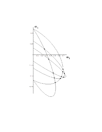
Figure 9: Topological structure of the inner resonances on the frequency plane $(\omega_{3},\omega_{2})$ plotted for different resonances: $(n_{2}=n_{1},n_{3}=n_{1}),~{}~{}~{}(n_{2}=2n_{1},n_{3}=3n_{1}),~{}~{}~{}(n_{2}=3n_{1},n_{3}=n_{1}),~{}~{}~{}(n_{2}=5n_{1},n_{3}=7n_{1}).$ Further values: $J=0.2,\,\,\,\,\,\,2\beta=0.3$.

In the general dimensional case ($N>>1$), the geometrical interpretation is less illustrative and much more complicated. Since we have to deal with $N-1$ dimensional hyper-curves in the N dimensional hyper-space, the basic concept is however the same [20]). This conclusion manifests fundamental features of the multidimensional nonlinear dynamical systems. The diffusive motion of the system in the stochastic net is named as Arnold diffusion. Therefore, the diffusion equation (16) is still justified. However, the coefficient of diffusion for Arnold diffusion is defined by an expression other than eq. (16), namely Sagdeev :

$$D_{A}=E^{2}\,\varepsilon\,H_{0z}\,e^{-{1}/{\varepsilon^{a(N)}}}.$$ (37)

Here $E$ is the system’s energy, $a(N)$ is a dimensional dependent scaling constant with an upper limit determined by the Arnold inequality relation [6]

$$a(N)<\frac{2}{6N(N-1)+3N+14}.$$ (38)

Obviously, for $N>>1$ , $a(N)\mapsto 0$ and the coefficient of the Arnold diffusion takes the more simple form

$$D_{A}=\frac{1}{e}\varepsilon E^{2}H_{0z}.$$ (39)

Comparing eq. (39) with the diffusion coefficient obtained for the case of two spins, i.e. eq. (16) we find

$$\frac{D_{A}}{D}=\frac{4E^{2}H_{0z}}{e\varepsilon T}.$$ (40)

This relation is important in that it delivers information on when the mechanism of stochastic switching and dynamical freezing are more efficient $\frac{D_{A}}{D}>1$ for a long spin chain, as compared to the case of a pair of spins.

II.6 Role of anisotropy field

Here we discuss the connection between the anisotropy field and Arnold diffusion. For the Arnold diffusion to occur the Jacobi matrix has to be none-degenerate. We note however, that the Jacobi matrix becomes degenerate in some cases if the anisotropy field is absent, as can be inferred from the structure of the Jacobi matrix. For example in the simplest case of three spins ,

$$\det\left|{\frac{{\partial^{2}H_{0}}}{{\partial S_{i}^{z}\partial S_{j}^{z}}}}\right|=-4J^{2}\beta+8\beta^{3}\neq 0,\,\,\,\,\,\,\,\,\,\,\,\,\,if\,\,\,\,\,\,\,\,\,\beta\neq 0.$$

Evaluating the determinant for different number of spins we find that with the anisotropy field being applied it is always non-degenerated, while for particular $N$, it becomes degenerated in absence of the anisotropy field.

III Low temperature limit

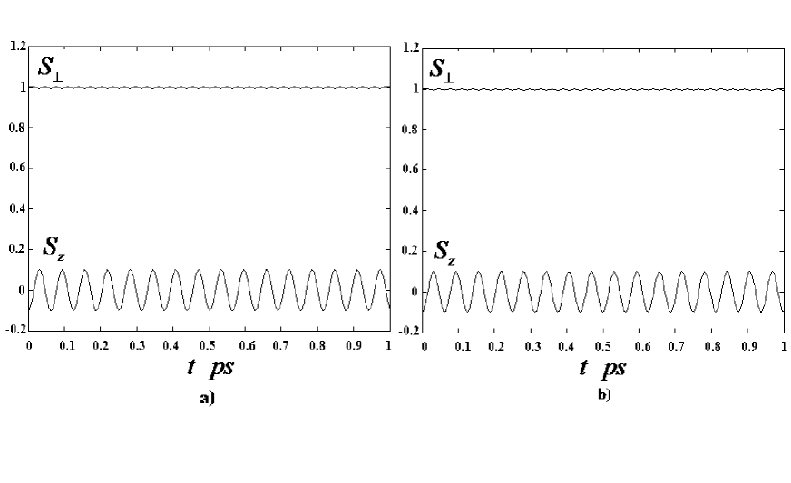
Figure 10: The longitudinal $s_{z}$, and the transversal $s_{\perp}=\sqrt{s_{x}^{2}+s_{y}^{2}}$ spin components as a function of time. $J=0.05$ ,  $H_{0z}=1$, $H_{0x}=0.1$. Graph a) shows the analytical solutions given by eq.(52), whereas in graph b) the numerical integration of the system of equations (III) is depicted.

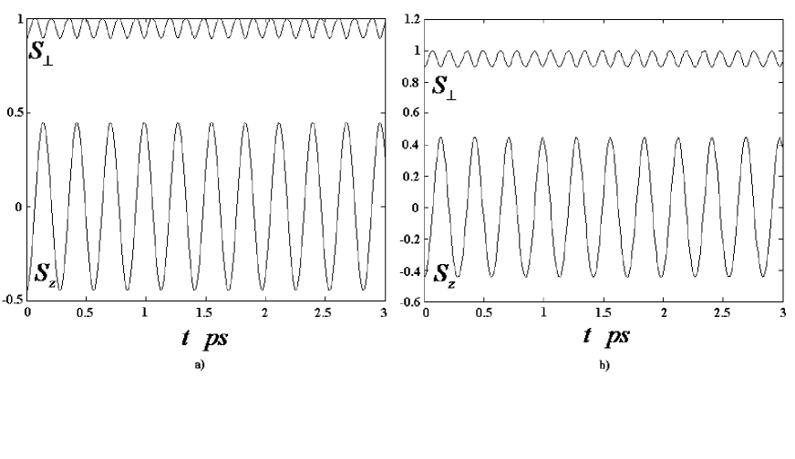
Figure 11: The same as in Fig.10 with the same meaning of the labels. The parameters of the system are however changed to $J=0.05$ ,$H_{0z}=0.2$, $H_{0x}=0.1$.

In this section we consider the dynamics in the continuous limit. By a proper choice of pulse parameters we were able to deflect the spin orientation diffusively to a desired angle. Switching off the pulses, the dynamics remain quasi frozen (is equivalent to the spin $z$ component being an integral of motion). The question we pose here is that what happens if upon stochastic switching and freezing we apply a constant magnetic field along $x$ axis. We recall that applying a constant field to the equilibrium (initial) state along the $x$ axis invalidates the use of the KAM theory and the mechanism of SC does not work (cf.eq.(II.1)). Before we deal with this problem in more details we set the limits of continuous approximation. Due to the constant magnetic field, applied along the $x$ axis, the $s_{z}$ component is not an integral of motion any more. Therefore, excitations similar to spin waves propagate along the spin chain. These waves are not completely analogous to spin waves because the non-conservation of $s_{z}(t)$ is not related to flip-flop processes, but requires a transversal magnetic field. However, the wavelength of such excitations can be evaluated in a manner similar to the spin waves case Kittel . If the wavelength is larger than the distance between the spins $\lambda>>a$ a continuous treatment is justified. Taking into account the expression for the wave frequency

$$\omega=\frac{4|J|S}{\hbar}\cdot\frac{2\pi}{\lambda}\cdot a,$$ (41)

One concludes that the validity of the continuous approximation depends on the temperature

$$T<<\frac{J\hbar}{k_{B}}.$$ (42)

Here $k_{B}$ is the Boltzmann constant. Thus, the continuous approximation corresponds to a low temperature approximation. For anti-ferromagnetic materials FeCl₂, or CoCl₂ we have $J=1.23\cdot 10^{12}$ Hz, from (42) we infer for temperature regime of the continuous model $T<3K$.

Returning back to the spin chain in a static magnetic field along $x$ axis, the EOM read

$$\frac{ds_{jx}}{dt}=-J\big{(}s_{j-1,z}+s_{j+1,z}\big{)}s_{jy}-H_{0z}s_{jy},$$

$$\frac{ds_{jy}}{dt}=J\big{(}s_{j-1,z}+s_{j+1,z}\big{)}s_{jx}+H_{0z}s_{jx}-H_{0x}s_{jz},$$ (43)

$$\frac{ds_{jz}}{dt}=H_{0x}s_{jy}.$$

Considering that

$$s_{jx}\rightarrow s_{x}(x;t),$$

$$s_{jy}\rightarrow s_{y}(x;t),$$ (44)

$$s_{jz}\rightarrow s_{z}(x;t)$$

$$s_{j-1;z}=s_{x}(x,t)-a\frac{\partial s_{z}(x,t)}{\partial x}+\frac{a^{2}}{2}\frac{\partial^{2}s_{x,t}}{\partial t^{2}},$$

$$s_{j+1;z}=s_{x}(x,t)+a\frac{\partial s_{z}(x,t)}{\partial x}+\frac{a^{2}}{2}\frac{\partial^{2}s_{x,t}}{\partial t^{2}},$$ (45)

from (43) we deduce that

$$\frac{\partial s_{x}}{\partial t}=-Js_{y}\bigg{(}2s_{z}+\frac{\partial^{2}s_{z}}{\partial x^{2}}a^{2}\bigg{)}-H_{0z}s_{y},$$

$$\frac{\partial s_{x}}{\partial t}=Js_{x}\bigg{(}2s_{z}+\frac{\partial^{2}s_{z}}{\partial x^{2}}a^{2}\bigg{)}-H_{0x}s_{z}+H_{0z}s_{x},$$ (46)

$$\frac{\partial s_{z}}{\partial t}=H_{0x}s_{y}.$$

In the low temperature regime we can neglect quadratic terms in (46) and obtain

$$\dot{x}=-\delta y-\gamma yz,$$

$$\dot{y}=\delta x-z+\gamma xz,$$ (47)

$$\dot{z}=y.$$

Here we introduced the following notations

$$\delta=\frac{H_{0z}}{H_{0x}},~{}~{}\gamma=\frac{2J}{H_{0x}},~{}~{}t\rightarrow H_{0x}t,~{}~{}s_{x}=x,~{}~{}s_{y}=y,~{}~{}s_{z}=z.$$

Eq.(47) is derived in the absence of anisotropy field. However for the role of the anisotropy field we remark the following: The Zeeman field applied along the $z$ axis is very strong $H_{0}^{z}>J\left|{S_{i-1}^{z}}\right|\,+J\left|{S_{i+1}^{z}}\right|+2\beta\left|{S_{i}^{z}}\right|$. The eigenfrequency is constant and we have no effect of a dynamical shift $\omega_{i}\left({S_{i-1}^{z}\,,S_{i+1}^{z},\,\,S_{i}^{z}}\right)=JS_{i-1}^{z}\,+JS_{i+1}^{z}+2\beta S_{i}^{z}+H_{0}^{z}\approx H_{0}^{z}$. Inclusion of a finite anisotropy field leads to a rescaling of the small parameter $\gamma$ in in Eq. (47), i.e. $\gamma=\frac{{2J}}{{H_{0x}}}\to\frac{{2J+2\beta}}{{H_{0x}}}$. Hence, we conclude that in this particular case the anisotropy field has no principal dynamical effect. Eq.(47) with rescaled parameter $\gamma=\frac{2J+2\beta}{H_{0x}}$ is still valid in the presence of anisotropy field.

When solving (47), we assume for the initial values the spin orientations achieved after action of pulses. In order to obtain analytical solutions we utilize the canonical perturbation theory (cf., e.g. Ugulava ). The parameter $\gamma$ is assumed to be small. First step is to rewrite (47) in a canonical form. This can be done using the following transformation. (For details, see Appendix)

$$x_{1}=2\delta x-2z,$$

$$y_{1}=2\lambda y,$$ (48)

$$z_{1}=\frac{1}{\delta}x+z,$$

$$\lambda=\sqrt{1+\delta^{2}},$$

Equations (47) assume then the form

$$\dot{x_{1}}=-\lambda y_{1}+\frac{\delta\gamma}{2\lambda^{3}}y_{1}x_{1}-\frac{\gamma\delta^{3}}{\lambda^{3}}y_{1}z_{1},$$

$$\dot{y_{1}}=\lambda x_{1}+\frac{\gamma\delta(\delta^{2}-1)}{\lambda^{3}}x_{1}z_{1}-\frac{\gamma\delta}{2\lambda^{3}}x_{1}^{2}+\frac{2\gamma\delta^{3}}{\lambda^{3}}z_{1}^{2},$$ (49)

$$\dot{z_{1}}=\frac{\gamma}{4\lambda^{3}\delta}y_{1}x_{1}-\frac{\gamma\delta}{2\lambda^{3}}y_{1}z_{1}.$$

We seek a solution of (49) having the structure

$$x_{1}=Cx_{1}^{1}+C^{2}x_{1}^{(2)}+C^{3}x_{1}^{(3)}+C^{4}x_{1}^{(4)}\ldots,$$

$$y_{1}=Cy_{1}^{1}+C^{2}y_{1}^{(2)}+C^{3}y_{1}^{(3)}+C^{4}y_{1}^{(4)}\ldots,$$ (50)

$$z_{1}=Cz_{1}^{1}+C^{2}z_{1}^{(2)}+C^{3}z_{1}^{(3)}+C^{4}z_{1}^{(4)}\ldots,$$

and in addition we use the re-scaled time

$$t=\frac{\tau}{\lambda}\big{(}1+h_{2}C^{2}+h_{3}C^{3}+\ldots\big{)}.$$ (51)

With an accuracy up to third order in $\gamma$ we find the solution of (47) to be

$$s_{x}=\frac{\delta\cos\tau}{\lambda}+\frac{\gamma(1+2\delta^{2})\sin^{2}(\tau)}{2\lambda^{4}}-\frac{\gamma^{2}\delta(9+4\delta^{2})\cos(\tau)\sin^{2}(\tau)}{16\lambda^{7}},$$

$$s_{y}=\sin(\tau)-\frac{\gamma\delta\cos(\tau)\sin(\tau)}{\lambda^{3}}+\frac{\gamma^{2}(1+4\delta^{2})(-5\sin(\tau)+3\sin(3\tau))}{64\lambda^{6}},$$ (52)

$$s_{z}=-\frac{\cos\tau}{\lambda}-\frac{\gamma\delta\sin^{2}(\tau)}{2\lambda^{4}}-\frac{\gamma^{2}(-1+4\delta^{2})\cos(\tau)\sin^{2}(\tau)}{16\lambda^{7}}.$$

Fig.10 demonstrate that these analytical solutions are in a good agreement with the exact numerical simulation of the system (III). Fig. 10 evidences that a constant magnetic field results in oscillations of spin’s longitudinal component in a controlled manner. If the amplitude of the magnetic field is small, nonlinear effects become more important (cf Fig.11).

IV Quantum Mechanical consideration and problem of DF

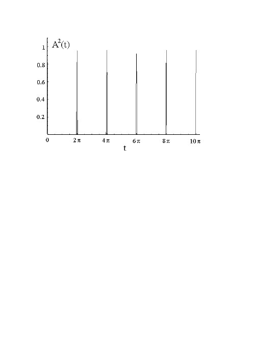
Figure 12: Bargmann angle $\theta_{B}(t)$ as a function of re-scaled time $t\equiv t/(H_{0z}+J)$, $H_{0z}=J=0,2$ calculated from (59).

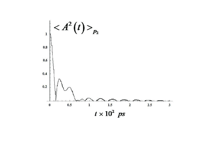
Figure 13: The time evolution of the Bargmann angle $\theta_{B}(t)$, as calculated using eq.(62) and averaged over the random quantum phases. The parameters of the driving fields and the spin chains are the same as in Fig.2, i.e. we are in the stochastic switching regime.

As stated above, the classical analysis is useful if the atoms in the chain have a large magnetic moment. In fact, for a finite chain of manganese (Mn) atoms science the classical approach proved to be adequate spintheory . This situation changes however, for small spins where the dynamics becomes dominated by quantum effects. What is needed for our quantum consideration is the structure of the energy spectrum in the regime where the underlying classical dynamics is chaotic Mejia-Monasterio . The point of interest here is that whether quantum effects invalidate the SC and in particular die dynamical freezing. To this end we use the concept of quantum geometry Pati ; vonBalk in the way done in Refs.[Matos-Abiague, ; Matos-Abiague2, ] to study DF. Let us consider two quantum states $\Psi_{1}$ and $e^{i\varphi}\Psi_{1}$. The distance in Hilbert space between them can be characterized by the quantity Pati ; Anandan ; vonBalk

$$D_{1}(\Psi_{1},\Psi_{2})=min_{\varphi}\big{\|}\Psi_{1}-e^{i\varphi}\Psi_{2}\big{\|}.$$

The minimal phase $\varphi_{m}$ is found by exterimizing $\big{\|}\Psi_{1}-e^{i\varphi}\Psi_{2}\big{\|}$ and noting that $\big{\|}\Psi_{1}-\Psi_{2}\big{\|}=\big{\langle}\Psi_{1}\big{|}\Psi_{2}\big{\rangle}^{1/2},$ which yields

$$\exp\big{(}i\varphi_{m}\big{)}=\frac{\big{\langle}\Psi_{1}\big{|}\Psi_{2}\big{\rangle}}{\big{|}\big{\langle}\Psi_{1}\big{|}\Psi_{2}\big{\rangle}\big{|}}.$$ (53)

Therefore, we writes for the distance $D_{1}$

$$D_{1}(\Psi_{1},\Psi_{2})=\sqrt{2-2\big{|}\big{\langle}\Psi_{1}\big{|}\Psi_{2}\big{\rangle}\big{|}}.$$

For the same purpose as for $D_{1}$, one may also use the Fubini-Study metric Anandan

$$D_{2}^{2}\big{(}\Psi(t),\Psi(0)\big{)}=4\big{(}1-\big{|}\big{\langle}\Psi(t)\big{|}\Psi(0)\big{\rangle}\big{|}^{2}\big{)}.$$ (54)

In both approaches the key quantity is the so-called Bargmann angle Matos-Abiague

$$\cos\theta_{B}(t)=A(t)=\big{|}\big{\langle}\Psi(0)\big{|}\Psi(t)\big{\rangle}\big{|}.$$ (55)

In analogy to the classical deflection in quantum control problems, the Bargmann angle can be considered as the ”quantum deflection”. Essential for further progress is our (classical) finding that SC and DF occur in the classical chaotic regime. This calls for the use of random matrix theory (RMT) to inspect the quantum dynamics Stockman ; Haake . To this end we write (2) as

$$\hat{H}(t)=\hat{H}_{0}+\hat{V}(t),$$ (56)

where $\hat{H}_{0}$ is time independent. Now we employ the established Floquet-operator method Haake and the quantum map and infer for the Bargmann angle

$$A^{2}(t)=\frac{1}{N^{2}}\bigg{(}N+\sum\limits_{n,m=1\atop n\neq m}^{N}\cos\big{[}t(\varphi_{n}-\varphi_{m})\big{]}\bigg{)}.$$ (57)

Here $\varphi_{n}$ stand for the eigen phases of the Floquet operators. $N$ is the Hilbert space dimension. From this relation it is evident that starting at $t=0$ with two completely coherent states, i.e. $A(t=0)=1$, de-coherence sets in for $t\neq 0$. To put the classical predictions of the previous section into a quantum perspective we note the following: In the classical regular regime, as identified above, the time-dependent perturbation $\hat{V}(t)$ acts adiabatically and does not alter the structure or the symmetry of the quantum spectrum. In this case we expect the Bargmann angle to be time periodic with typical quantum revivals. In contrast, in the classical chaotic regime, $\hat{V}(t)$ changes qualitative the quantum spectrum.

Starting from the (classically) regular case we conclude that, if pair excitations are neglected, then the energy spectrum of the unperturbed part has the form

$$E_{n}=(n-1-N/2)H_{0z}+\frac{1}{4}J(N-4n+3)+\frac{\beta N}{4}.$$ (58)

With this spectrum we infer for the Bargmann angle (eq.(57)) the expression

$$A^{2}(t)=\frac{1}{N^{2}}\bigg{(}\frac{\sin(N+1/2)t-\sin(t/2)}{2\sin(t/2)}\bigg{)}^{2}+\frac{1}{N^{2}}\bigg{(}\frac{\cos(t/2)-\cos(N+1/2)t}{2\sin(t/2)}\bigg{)}^{2}.$$ (59)

As evident from Fig.11, if the underlying classical dynamics is regular, the time dependence of the Bargmann angle is periodical and the system is characterized by quantum revivals.

To deal quantum mechanically with the classically chaotic regime we follow Ref. Haake and employ a Gaussian orthogonal ensemble Haake .

$$P(\varphi_{1},\ldots\varphi_{N})=\prod\limits_{n>m}(\varphi_{n}-\varphi_{m})\exp\bigg{(}-\sum\limits_{n=1}^{N}\varphi_{n}^{2}\bigg{)}.$$ (60)

We note here that in general the distribution function (60) includes correlations between all $N$ levels. If the number of correlated levels is $n$, then the $n<N$ level-correlated distribution function reads

$$P_{n}(\varphi_{1},\ldots\varphi_{n})=\frac{N!}{(N-n)!}\int P_{n}(\varphi_{1},\ldots\varphi_{N})d\varphi_{n+1}\ldots d\varphi_{N}.$$ (61)

The structure of the expression (57) suggests that the second-order correlated level distribution function $P_{2}(\varphi_{n},\varphi_{m})$ is sufficient (each term in the sum contains two phases). Upon straightforward calculations we reduced $P_{2}(\varphi_{n},\varphi_{m})$ to

$$P_{2}(\varphi_{n},\varphi_{m})=K_{N}(\varphi_{n},\varphi_{n})K_{N}(\varphi_{m},\varphi_{m})-K_{N}(\varphi_{n},\varphi_{m})K_{N}(\varphi_{m},\varphi_{n}),$$

with

$$K(\varphi_{n},\varphi_{m})=\sum\limits_{k=1}^{N}\phi_{k}(\varphi_{n})\phi_{k}(\varphi_{n}),$$

and

$$\phi_{k}(\varphi)=\frac{1}{\big{(}2^{n}n!\sqrt{\pi}\big{)}^{1/2}}H_{k}(\varphi)\exp\bigg{[}-\frac{\varphi^{2}}{2}\bigg{]}.$$

$H_{n}(\varphi)$ are Hermite polynomials. For $\big{\langle}A^{2}(t)\big{\rangle}_{P_{2}}$ we find (for $N\gg 1$)

$$\big{\langle}A^{2}(t)\big{\rangle}_{P_{2}}=C\exp\big{[}-t^{2}/2\big{]}\bigg{\{}\sum\limits_{n,m}^{N}L_{n}^{0}\big{(}t^{2}/2\big{)}L_{m}^{0}\big{(}t^{2}/2\big{)}-\frac{\sqrt{\pi}}{4}\sum\limits_{m=1}^{N}\sum\limits_{n=1}^{N}\frac{n!}{2^{m-n}m!}t^{m-n}$$

$$\big{(}L_{n}^{m-n}\big{(}t^{2}/2\big{)}\big{)}^{2}-\frac{\sqrt{\pi}}{4}\sum\limits_{m=1}^{N}\sum\limits_{n=1}^{m-1}\frac{n!}{2^{m-n}m!}t^{m-n-1}\big{(}L_{n}^{m-n-1}\big{(}t^{2}/2\big{)}\big{)}^{2}\bigg{\}}$$ (62)

where $L_{n}^{m}(t^{2}/2)$ are Laguerre polynomials. The constant $C$ we find from the condition $\big{\langle}A^{2}(0)\big{\rangle}_{P_{2}}=1$. Dynamical freezing (DF) means then a stabilization over time of the quantum distance Matos-Abiague2 ; Matos-Abiague quantified by the Bargmann angle. To test for this situation we numerically solve for (62); a typical example is shown in Fig.(13). These calculations are performed for parameters appropriate for the classically chaotic regime, e.g. those of Fig.2. The interpretation of Fig.(13) is that SC drives the system diffusively to the target state $\big{|}\Psi(t)\big{\rangle}$, which in this case is orthogonal to $\big{|}\Psi(0)\big{\rangle}$. The Bargmann angle is therefore deflected within a time $t_{D}$ determined by the diffusion constant to the value $\theta_{B}(t_{D})\sim\pi/2$. DF is then evidenced by a small variations of $\theta_{B}(t_{D})$ for $t>t_{D}$.

IV.1 Conclusions

For an exchange-coupled, non-linear spin chain and in the presence of a (uniaxial) magnetic anisotropy and external driving fields, stochastic switching is possible if the field parameters are chosen such that the underlying classical dynamics is chaotic. The switching mechanism is identified to be the Arnold-type diffusion. This we concluded analytically and substantiated by full numerical semi-classical and quantum calculations. We also inspected the possibility of dynamical freezing, i.e. stabilizing the target state beyond the switching time.

Acknowledgment: The project is financially supported by the Georgian National Foundation (grants: GNSF/STO 7/4-197, GNSF/STO 7/4-179). The financial support by the Deutsche Forschungsgemeinschaft (DFG) through SFB 762 and though SPP 1285 is gratefully acknowledged.

Appendix A

The canonical Lyapunov system has the general structure

$$\dot{x}=-\lambda y+X(x,y,z_{1}\ldots z_{m});$$

$$\dot{y}=\lambda x+Y(x,y,z_{1}\ldots z_{m});$$ (63)

$$\dot{z}_{s}=\sum\limits_{j=1}^{m}b_{sj}+Z_{s}(x,y,z_{1}\ldots z_{m});$$

$$(s=1,2,\ldots m;m=n-2)$$

We seek a reduction of this system of equations using the canonical transformation

$$\dot{x}=-\delta y-\gamma yz,$$

$$\dot{y}=\delta x-z+\gamma xz,$$ (64)

$$\dot{z}=y.$$

We are interested in the linear part of eq. (A), i.e.

$$\dot{x}=-\delta y,$$

$$\dot{y}=\delta x-z,$$ (65)

$$\dot{z}=y,$$

From the coefficients of the equation (A) we can construct the following matrix

$$a=\left(\begin{array}[]{c}0~{}~{}-\delta~{}~{}0\\ \delta~{}~{}0~{}~{}-1\\ 0~{}~{}1~{}~{}0\end{array}\right).$$ (66)

We consider now the linear transformation

$$\xi_{1}=\gamma_{11}x+\gamma_{12}y+\gamma_{13}z,$$

$$\xi_{2}=\gamma_{21}x+\gamma_{22}y+\gamma_{23}z,$$ (67)

$$\xi_{3}=\gamma_{31}x+\gamma_{32}y+\gamma_{33}z.$$

In the new variables eq. (A3) is cast as

$$\frac{d\xi_{i}}{dt}=\lambda_{i}\xi_{i}~{}~{}~{}~{}i=1,2,3.$$ (68)

Taking eqs.(A), (A) into account we infer from eq. (68) that

$$(a_{11}-\lambda_{i})\gamma_{i1}+a_{21}\gamma_{i2}+a_{31}\gamma_{i2}=0,$$

$$a_{12}\gamma_{i1}+(a_{22}-\lambda_{i})\gamma_{i2}+a_{32}\gamma_{i3}=0,$$ (69)

$$a_{13}\gamma_{i1}+a_{23}\gamma_{i2}+(a_{33}-\lambda_{i})\gamma_{i3}=0.$$

Equating the determinant to zero

$$\left|\begin{array}[]{c}-\lambda_{i}~{}~{}-\delta~{}~{}0\\ \delta~{}~{}-\lambda_{i}~{}~{}-1\\ 0~{}~{}1~{}~{}-\lambda_{i}\end{array}\right|=0,$$ (70)

we find

$$\lambda_{1,2}=\pm i\lambda,~{}~{}\lambda_{3}=0,~{}~{}\lambda=\sqrt{1+\delta^{2}}.$$ (71)

According to (A) this gives the following solutions for the matrix

$$\gamma_{11}=-\delta,~{}~{}-\gamma_{12}=-i\lambda,~{}~{}\gamma_{13}=1;$$

$$\gamma_{21}=-\delta,~{}~{}-\gamma_{22}=-i\lambda,~{}~{}\gamma_{23}=1;$$ (72)

$$\gamma_{31}=-\frac{1}{\delta},~{}~{}-\gamma_{22}=0,~{}~{}\gamma_{33}=1.$$

So the canonical transformation (A) has the form

$$\xi_{1}=-\delta x-i\lambda y+z;$$

$$\xi_{2}=-\delta x+i\lambda y+z;$$ (73)

$$\xi_{3}=-\frac{1}{\delta}x+z.$$

The inverse transformation reads

$$x=\frac{\delta}{\lambda^{2}}\bigg{(}\xi_{3}-\frac{\xi_{1}+\xi_{2}}{2}\bigg{)},$$

$$y=\frac{i}{2\lambda}(\xi_{1}+\xi_{2}),$$ (74)

$$z=\frac{\xi_{1}+\xi_{2}+2\delta^{2}\xi_{3}}{2\lambda^{2}}.$$

Using eq.(A) we obtain then for equations of motion in the variable $\xi_{i}$

$$\dot{\xi}_{1}=i\lambda\xi_{1},$$

$$\dot{\xi}_{2}=-i\lambda\xi_{2},$$

$$\dot{\xi}_{3}=0.$$

To reduce our system of equations to the canonical form, one more transformation is needed

$$x_{1}=-(\xi_{1}+\xi_{2}),$$

$$y_{1}=i(\xi_{1}-\xi_{2}),$$ (76)

$$z_{1}=\xi_{3}.$$

Taking eqs.(A) , (A) into account we obtain

$$x_{1}=2\delta x-2z;$$

$$y_{1}=2\lambda y;$$ (77)

$$z_{1}=\frac{1}{\delta}x+z.$$

The inverse transformation reads

$$x=\frac{\delta}{\lambda^{2}}\bigg{(}z_{1}+\frac{x_{1}}{2}\bigg{)},$$

$$y=\frac{1}{2\lambda}y_{1},$$ (78)

$$z=\frac{1}{\lambda^{2}}\big{(}-x_{1}+2\delta^{2}z_{1}\big{)}.$$

Using (A), (A) we can finally rewrite the set of equations in the canonical form

$$\dot{x_{1}}=-\lambda y_{1}+\frac{\delta\gamma}{2\lambda^{3}}y_{1}x_{1}-\frac{\gamma\delta^{3}}{\lambda^{3}}y_{1}z_{1},$$

$$\dot{y_{1}}=\lambda x_{1}+\frac{\gamma\delta(\delta^{2}-1)}{\lambda^{3}}x_{1}z_{1}-\frac{\gamma\delta}{2\lambda^{3}}x_{1}^{2}+\frac{2\gamma\delta^{3}}{\lambda^{3}}z_{1}^{2},$$ (79)

$$\dot{z_{1}}=\frac{\gamma}{4\lambda^{3}\delta}y_{1}x_{1}-\frac{\gamma\delta}{2\lambda^{3}}y_{1}z_{1}.$$

References

- (1) C. F. Hirjibehedin, C. P. Lutz, and A. J. Heinrich, Science 312, 1021 (2006); S. Rusponi et al., Nature Mater. 2, 546 (2003); T. Mirkovic et al., Nature Nanotech. 2, 565 (2007); J. A. Stroscio and R. J. Celotta, Science 306, 242 (2004).
- (2) S. Lounis, Ph. Mavropoulos, P. H. Dederichs, and S. Blügel, Phys. Rev. B 72, 224437 (2005); S. Lounis, P. H. Dederichs, and S. Blügel, Phys. Rev. Lett. 101, 107204 (2008); P. Politi and M. Gloria Pini 79, 012405 (2009) and references therein.
- (3) A. Abragam and M. Goldman Nuclear Magnetism: Order and Disorder (Oxford: Oxford University Press) (1982)
- (4) C. Mejia-Monasterio, T. Prosen, and G. Gasati, Europhys.Lett. 72 (4), p.520, (2005)
- (5) K. Saito,Europhys.Lett. 61, 34 (2003)
- (6) G.M. Zaslavsky, The physics of chaos in hamiltonian systems 2ed edition, (Imperial College London, 2007).
- (7) L. L.Chotorlishvili, V. M. Ckhvaradze Low.Temp.Physics v. 30, No. 9, p. 739 (2004)
- (8) A. Matos-Abiague and J. Berakdar Phys.Rev A 73, 024102 (2006)
- (9) A. Matos-Abiague and J. Berakdar Euro. Phys. Lett 71, 705-711 (2005)
- (10) Xiao-Zhong Yuan, Hsi-Sheng Goan, and Ka-Di Zhu, Phys.Rev. B 75, 045331 (2007).
- (11) Q.A. Tuchette et al., Phys.Rev.Lett. 75, 4710 (1995).
- (12) H. Mabuchi and A. Doherty, Science 298, 1372 (2002).
- (13) C.J. Hood et al., Science 287, 1447 (2000).
- (14) J.Raimond,M.Brune, and S.Haroche, Rev.Mod.Phys. 73, 565 (2001).
- (15) L.Chotorlishvili, Z. Toklikishvili, Phys.Lett.A v. 372, 2806 (2008)
- (16) M. Lakshmanan and A. Saxena arXiv: 0712.2503v1, (2007)
- (17) Y. Zolotaryuk, S. Flach, and V. Fleurov, Phys.Rev.B, 214422, (2001)
- (18) A. Sukhov, J. Berakdar Phys.Rev.Lett. 102, 057204 (2009)
- (19) R. Balescu. Equilibrium and Nonequilibrium Statistical Mechanics. (New York, Wiley, 1975.)
- (20) A. J. Lichtenberg and M.A. Lieberman, Regular and Chaotic Dynamics (Springer-Verlag, New York, 1992),
- (21) H. Haken, Synergetics. An Introduction, Berlin: Springer-Verlag, 1978.
- (22) L.Chotorlishvili, Z. Toklikishvili, J. Berakdar Phys.Lett.A 373, 231 (2009)
- (23) B. V. Chirikov. Physics Reports, Volume 52, Issue 5, May 1979, Pages 263-379
- (24) Ch. Kittel, Introduction to Solid State Physics, Fourth Edition, John Wiley and Sons, (New York, London, Sydney, Toronto, 1978),
- (25) A. I. Ugulava, L. L. Chotorlishvili, Z. Z. Toklikishvili, and A. V. Sagaradze, Low.Temp.Physics, v.32, No. 10, p. 915, (2006)
- (26) A. K. Pati and S. V. Lawande, Phy. Rev. A v.58, No. 2, 831, (1998)
- (27) J. Anandan, Y. Aharonov Phys.Rev.Lett. v.65, N. 14, p. 1697 (1990)
- (28) R. von Balk, Eur. J Phys 11 215-220, (1990)
- (29) H.J. Stöckmann, Quantum Chaos, An Introduction (Cambridge Univ.Press, Cambridge, 1993).
- (30) F.Haake, Quantum Signatures of Chaos (Springer, Berlin,2001).
- (31) L. Chotorlishvili, V. Skrinnikov Phys. Lett. A 372, 761-768, (2008)