Abstract

A new class of LRS Bianchi type ${\rm VI}_{0}$ cosmological models with free gravitational fields and a variable cosmological term is investigated in presence of perfect fluid as well as bulk viscous fluid. To get the deterministic solution we have imposed the two different conditions over the free gravitational fields. In first case we consider the free gravitational field as magnetic type whereas in second case ‘gravitational wrench’ of unit ‘pitch” is supposed to be present in free gravitational field. The viscosity coefficient of bulk viscous fluid is assumed to be a power function of mass density. The effect of bulk viscous fluid distribution in the universe is compared with perfect fluid model. The cosmological constant $\Lambda$ is found to be a positive decreasing function of time which is corroborated by results from recent observations. The physical and geometric aspects of the models are discussed.

PACS: 98.80.Cq, 98.80.-k
Keywords: Cosmology, Bianchi models, Gravitational Fields, Bulk Viscosity

1 Introduction and Motivations

The cosmological constant($\Lambda$) was introduced by Einstein in 1917 as the universal repulsion to make the Universe static in accordance with generally accepted picture of that time. In absence of matter described by the stress energy tensor $T_{ij}$, $\Lambda$ must be constant, since the Bianchi identities guarantee vanishing covariant divergence of the Einstein tensor, $G^{ij}_{;j}=0$, while $g^{ij}_{;j}=0$ by definition. If Hubble parameter and age of the universe as measured from high red-shift would be found to satisfy the bound $H_{0}t_{0}>1$ (index zero labels values today), it would require a term in the expansion rate equation that acts as a cosmological constant. Therefore the definitive measurement of $H_{0}t_{0}>1$ would necessitate a non-zero cosmological constant today or the abandonment of the standard big bang cosmology [1]. The idea that $\Lambda$ might be variable has been studied for more than two decades (see [2, 3] and references therein). Linde [4] has suggested that $\Lambda$ is a function of temperature and is related to the process of broken symmetries. Therefore, it could be a function of time in a spatially homogeneous, expanding universe [3]. In a paper on $\Lambda$- variability, Overduin and Cooperstock [5] suggested that $\Lambda g_{ij}$ is shifted onto the right-hand side of the Einstein field equation and treated as part of the matter content. In general relativity, $\Lambda$ can be regarded as a measure of the energy density of the vacuum and can in principle lead to the avoidance of the big bang singularity that is characterized of other FRW models. However, the rather simplistic properties of the vacuum that follows from the usual form of Einstein equations can be made more realistic if that theory is extended, which in general leads to a variable $\Lambda$. Recently Overduin [6, 7] has given an account of variable $\Lambda$-models that have a non-singular origin. Liu and Wesson [8] have studied universe models with variable cosmological constant. Podariu and Ratra [9] have examined the consequences of also incorporating constraints from recent measurements of the Hubble parameter and the age of the universe in the constant and time-variable cosmological constant models.

A dynamic cosmological term $\Lambda(t)$ remains a focal point of interest in modern cosmological theories as it solves the cosmological constant problem in a natural way. There are significant observational evidence for the detection of Einstein’s cosmological constant, $\Lambda$ or a component of material content of the universe that varies slowly with time to act like $\Lambda$. In the context of quantum field theory, a cosmological term corresponds to the energy density of vacuum. The birth of the universe has been attributed to an excited vacuum fluctuation triggering off an inflationary expansion followed by the super-cooling. The release of locked up vacuum energy results in subsequent reheating. The cosmological term, which is measure of the energy of empty space, provides a repulsive force opposing the gravitational pull between the galaxies. If the cosmological term exists, the energy it represents counts as mass because mass and energy are equivalent. If the cosmological term is large enough, its energy plus the matter in the universe could lead to inflation. Unlike standard inflation, a universe with a cosmological term would expand faster with time because of the push from the cosmological term (Croswell [10]). In the absence of any interaction with matter or radiation, the cosmological constant remains a “constant”. However, in the presence of interactions with matter or radiation, a solution of Einstein equations and the assumed equation of covariant conservation of stress-energy with a time-varying $\Lambda$ can be found. This entails that energy has to be conserved by a decrease in the energy density of the vacuum component followed by a corresponding increase in the energy density of matter or radiation (see also Weinberg [11], Carroll et al. [12], Peebles [13], Sahni and Starobinsky [14], Padmanabhan [15, 16], Singh et al. [17], Pradhan and Pandey [18, 19], Pradhan and Singh [20], Pradhan et al. [21, 22]). Several authors (Pradhan [23, 24], Pradhan et al. [25]$-$[28], Abdussattar and Viswakarma [29], Kalita et al. [30], Pradhan & Jotania [31] have studied the cosmological models with decaying vacuum energy density $\Lambda$.

The discovery in 1998 that the Universe is actually speeding up its expansion was a total shock to astronomers. The observations for distant Type Ia supernovae (Perlmutter et al. [32]$-$[34] and Riess et al. [35, 36], Garnavich et al. [37, 38], Schmidt et al. [39]) in order to measure the expansion rate of the universe strongly favour a significant and positive value of $\Lambda$. These measurements, combined with red-shift data for the supernovae, led to the prediction of an accelerating universe. They obtained $\Omega_{M}\approx 0.3$, $\Omega_{\Lambda}\approx 0.7$, and strongly ruled out the traditional ($\Omega_{M},\Omega_{\Lambda}$) = ($1,0$) universe. This value of the density parameter $\Omega_{\Lambda}$ corresponds to a cosmological constant that is small, nevertheless, nonzero and positive, that is, $\Lambda\approx 10^{-52}m^{-2}\approx 10^{-35}s^{-2}$. An intense search is going on, in both theory and observations, to unveil the true nature of this acceleration. It is commonly believed by the cosmological community that a kind of repulsive force which acts as anti-gravity is responsible for gearing up the Universe some $7$ billion years ago. This hitherto unknown exotic physical entity is termed as dark energy. The simplest Dark Energy (DE) candidate is the cosmological constant $\Lambda$, but it needs to be extremely fine-tuned to satisfy the current value of the DE.

In classical electromagnetic theory, the electromagnetic field has two independent invariants $F_{ij}F^{ij}$ and ${}^{\ast}F_{ij}F^{ij}$. The classification of the field is characterized by the property of the scalar $k^{2}$ = $(F_{ij}F^{ij})^{2}$ + $(^{\ast}F_{ij}F^{ij})^{2}$. When $k$ = $0$, the field is said to be null and for any observer $|E|$ = $|H|$ and $E$.$H$ = 0 where E and H are the electric and magnetic vectors respectively. When $k$ $\neq{0}$, the field is non-null and there exists an observer for which $mE$ = $nH$, $m$ and $n$ being scalars. It is easy to see that if ${}^{\ast}F_{ij}F^{ij}$ = 0, $F_{ij}F^{ij}$ $\neq{0}$, then either $E$ = $0$ or $H$ = $0$. These we call the magnetic and electric fields, respectively. If $F_{ij}F^{ij}$ = $0$,${}^{\ast}F_{ij}F^{ij}$ $\neq{0}$ then $E$ = $\pm{H}$. This we call the ‘electromagnetic wrench’ with unit ‘pitch’. In this case Maxwell’s equations lead to an empty electromagnetic field with constant electric and magnetic intensities. In the case of gravitational field, the number of independent scalar invariants of the second order is fourteen. The independent scalar invariants formed from the conformal curvature tensor are four in number. In the case of Petrov type D space-times, the number of independent scalar invariants are only two, viz. $C_{hijk}C^{hijk}$ and ${}^{\ast}C_{hijk}C^{hijk}$. Analogous to the electromagnetic case, the electric and magnetic parts of free gravitational field for an observer with velocity $v^{i}$ are mentioned by Ellis [40] as $E_{\alpha\beta}=C_{\alpha j\beta i}v^{i}v^{j}$ and $H_{\alpha\beta}$ = ${}^{\ast}C_{\alpha j\beta i}v^{i}v^{j}$. It is clear from the canonical form of the conformal curvature for a general Petrov type D space-time that there exists an observer for which $E_{\alpha\beta}=(\frac{n}{m})H_{\alpha\beta}$, where $m,n$ being integers and $m\neq{0}$. The field is said to be purely magnetic type for $n=0$, $m\neq{0}$. In this case we have $E_{\alpha\beta}=0$ and $H_{\alpha\beta}\neq{0}$. The physical significance for the gravitational field of being magnetic type is that the matter particles do not experience the tidal force. When $m\neq{0}$ and also $n\neq{0}$, we call that there is a ‘gravitational wrench’ of unit ‘pitch’ $|\frac{n}{m}|$ in the free gravitational field [41]. If ‘pitch’ is unity then we have $E_{\alpha\beta}=\pm H_{\alpha\beta}$.

The space-time having a symmetry property is invariant under a continuous group of transformations. The transformation equations for such a group of order r is given by

$$X^{i}=f^{i}(x^{1},...,x^{r},a^{1},...,a^{r})$$ (1)

which satisfy the differential equations

$$\frac{{\partial}X^{i}}{{\partial}x^{\alpha}}=\xi^{i}_{(\beta)}(X)A^{\beta}_{\alpha}{(a)},~{}~{}(\alpha,\beta=1,...,r)$$ (2)

where $a^{1},...,a^{r}$ are r essential parameters. The vectors $\xi^{i}_{\alpha}$ are the Killing vectors for the group $G_{r}$ of isometry satisfying the Killing’s equation

$$\xi_{(\alpha)i;j}+\xi_{(\alpha)j;i}=0$$ (3)

A subspace of space-time is said to be the surface of transitivity of the group if any point of this space can be transformed to another point of it by the action of this group. A space-time is said to be spatially homogeneous if it admit a group $G_{r}$ of isometry which is transitive on three dimensional space-like hyper-surfaces. The group $G_{3}$ of isometry was first considered by Bianchi [42] who obtained nine different types of isometry group known as the Bianchi types. The space-time which admits $G_{4}$ group of isometry is known as locally rotationally symmetric (LRS) which always has a $G_{3}$ as its subgroup belonging to one of the Bianchi type provided this $G_{3}$ is simply transitive on the three dimensional hyper-surface $t$ = constant.

Considerable work has been done in obtaining various Bianchi type cosmological models and their inhomogeneous generalization. Barrow [43] pointed out that Bianchi ${\rm VI}_{0}$ models of the universe give a better explanation of some of the cosmological problems like primordial helium abundance and they also isotropize in a special sense. Looking to the importance of Bianchi type ${\rm VI}_{0}$ universes, many authors [44]$-$[48] have studied it in different context. Recently Bali et al. [49] have obtained some LRS Bianchi type ${\rm VI}_{0}$ cosmological models imposing two types of conditions over the free gravitational fields.

In this paper we have revisited and extended the work of Bali et al. [49] for bulk viscous fluid distribution. We have considered an LRS Bianchi type ${\rm VI}_{0}$ space-time and obtained models with free gravitational field of purely ‘magnetic type’ and also in the presence of ‘gravitational wrench’ of unit ‘pitch’ in the free gravitational field. It is found that the ‘magnetic’ part of the free gravitational field induces shear in the fluid flow, which is zero in the case of a ‘electric’ type free gravitational field representing an unrealistic distribution in this case. This paper is organized as follows. The introduction and motivation are laid down in Sec. $1$. The metric and the field equations are given in Sec. $2$. In Sec. $3$, solutions representing LRS Bianchi type ${\rm VI}_{0}$ cosmological models with perfect fluid and bulk viscous fluid are obtained imposing the condition when the free gravitational field is purely magnetic type ($m\neq 0,n=0$). In Sec. $4$, we obtain the solution in presence of perfect fluid imposing the condition when there is a ‘gravitational wrench’ of unit ‘pitch’ in the free gravitational field i.e. $E_{\alpha\beta}=\pm H_{\alpha\beta}$. Discussion and concluding remarks are given in the last Sec $5$.

2 The Metric and Field Equations

We consider an LRS Bianchi type ${\rm VI}_{0}$ universe for which

$$ds^{2}=\eta_{ab}\theta^{a}\theta^{b},$$ (4)

where $\theta^{1}=A(t)dx$, $\theta^{2}=B(t)\exp{(x)}dy$, $\theta^{3}=B(t)\exp{(-x)}dz$, $\theta^{4}=dt$.
The energy-momentum tensor for a perfect fluid distribution with comoving flow vector $v^{i}$ is given by

$$T^{j}_{i}=(\rho+p)v_{i}v^{j}+p\delta^{j}_{i},$$ (5)

where $v^{i}=\delta^{i}_{4}$, $\rho$ and $p$ being respectively, energy density and thermodynamic pressure of the fluid. Here we obtain

$$T^{1}_{1}=T^{2}_{2}=T^{3}_{3}=p,T^{4}_{4}=-\rho.$$ (6)

The Einstein’s field equations (in gravitational units c = 1, G = 1) read as

$$R^{j}_{i}-\frac{1}{2}R\delta^{j}_{i}+\Lambda\delta^{j}_{i}=-8\pi T^{j}_{i},$$ (7)

for the line element (4) has been set up as

$$\frac{2\ddot{B}}{B}+\frac{\dot{B}^{2}}{B^{2}}+\frac{1}{A^{2}}+\Lambda=-8\pi p,$$ (8)

$$\frac{\ddot{A}}{A}+\frac{\ddot{B}}{B}+\frac{\dot{A}\dot{B}}{AB}-\frac{1}{A^{2}}+\Lambda=-8\pi p,$$ (9)

$$\frac{2\dot{A}\dot{B}}{AB}+\frac{\dot{B}^{2}}{B^{2}}-\frac{1}{A^{2}}+\Lambda=8\pi\rho.$$ (10)

Here, and also in the following expressions a dot indicates ordinary differentiation with respect to $t$.

The energy conservation equation $T^{ij}_{;j}=0$, leads to the following expression

$$\dot{\Lambda}+\dot{\rho}+(\rho+p)\left(\frac{\dot{A}}{A}+2\frac{\dot{B}}{B}\right)=0.$$ (11)

The average scale factor $S$ for LRS Bianchi type ${\rm VI}_{0}$ model is defined by

$$S=(AB^{2})^{\frac{1}{3}}.$$ (12)

A volume scale factor is given by

$$V=S^{3}=(AB^{2}).$$ (13)

The generalized mean Hubble parameter $H$ is given by

$$H=\frac{1}{3}(H_{x}+H_{y}+H_{z}),$$ (14)

where $H_{x}=\frac{\dot{A}}{A}$, $H_{y}=H_{z}=\frac{\dot{B}}{B}$.

The expansion scalar $\theta$ and shear scalar $\sigma$ are obtained as

$$\theta=v^{i}_{;i}=\frac{\dot{A}}{A}+\frac{2\dot{B}}{B},$$ (15)

and

$$\sigma=\frac{1}{\sqrt{3}}\left(\frac{\dot{A}}{A}-\frac{\dot{B}}{B}\right),$$ (16)

respectively. The average anisotropy parameter is given by

$$A_{p}=\frac{1}{3}\sum_{i=1}^{3}{\left(\frac{\Delta{H_{i}}}{H}\right)^{2}},$$ (17)

where $\Delta{H_{i}}=H_{i}-H(i=1,2,3)$.
The deceleration parameter ($q$) is defined as

$$q=-\frac{\frac{\ddot{S}}{S}}{\frac{\dot{S}^{2}}{S^{2}}}.$$ (18)

The non-vanishing physical components of $C_{ijkl}$ for the line-element (4) are given by

$$C_{2323}=-\frac{1}{2}C_{3131}=C_{1212}=-C_{1414}=\frac{1}{2}C_{2424}=-C_{3434}$$

$$=\frac{1}{6}\left[\frac{2\ddot{A}}{A}-\frac{2\ddot{B}}{B}-\frac{2\dot{A}\dot{B}}{AB}+\frac{2\dot{B}^{2}}{B^{2}}+\frac{4}{A^{2}}\right],$$ (19)

$$C_{2314}=-\frac{1}{2}C_{3124}=C_{1234}=-\frac{1}{A}\left[\frac{\dot{A}}{A}-\frac{\dot{B}}{B}\right].$$ (20)

Equations (8)-(10) are three relations in five unknowns $A$, $B$, $p$, $\rho$ and $\Lambda$. For complete solutions of equations (8)-(10), we need two extra conditions. To simply the Einstein equations, we impose conditions on the Weyle tensor. Since the distribution of matter determines the nature of expansion in the model, the latter is also affected by the free gravitational field through its effect on the expansion, vorticity and shear in the fluid flow. A prescription of such a field may therefore be made on an a priori basis. The cosmological models of Friedman Robertson Walker, as well as the universe of Einstein-de Sitter, have vanishing free gravitational fields. In the following two cases we impose different conditions over the free gravitational field to find the deterministic solutions.

3 First Case: Free Gravitational Field is Purely Magnetic Type

3.1 Solution in Presence of Perfect Fluid

In this section we have extended the solution obtained by Bali et al. [49] by revisiting their solution. When free gravitational field is purely magnetic type ($m\neq 0,n=0$), we have $H_{\alpha\beta}\neq 0$ and $E_{\alpha\beta}=0$. From (19), we obtain

$$\frac{\ddot{A}}{A}-\frac{\ddot{B}}{B}-\frac{\dot{A}\dot{B}}{AB}+\frac{\dot{B}^{2}}{B^{2}}+\frac{2}{A^{2}}=0.$$ (21)

Equation (8) together with (9) reduce to

$$\frac{\ddot{A}}{A}-\frac{\ddot{B}}{B}+\frac{\dot{A}\dot{B}}{AB}-\frac{\dot{B}^{2}}{B^{2}}-\frac{2}{A^{2}}=0.$$ (22)

From Eqs. (21) and (22), we obtain two independent equations

$$\frac{\ddot{A}}{A}-\frac{\ddot{B}}{B}=0,$$ (23)

$$\frac{\dot{A}\dot{B}}{AB}-\frac{\dot{B}^{2}}{B^{2}}-\frac{2}{A^{2}}=0.$$ (24)

Let $\frac{A}{B}=U$. Then Eqs. (23) and (24) take the form

$$UU_{\xi\xi}+UU_{\xi}\dot{A}-2U^{2}_{\xi}=0,$$ (25)

and

$$U^{2}_{\xi}-UU_{\xi}\dot{A}+2U^{2}=0,$$ (26)

respectively, where $\xi$ is defined by

$$\frac{d}{dt}=\frac{1}{A}\frac{d}{d\xi}.$$ (27)

Eqs. (25) and (26) lead to

$$UU_{\xi\xi}-U^{2}_{\xi}+2U^{2}=0.$$ (28)

On substituting $U=\exp{(\mu)}$, the above second order differential equation reduces to the form

$$\mu_{\xi\xi}+2=0,$$ (29)

which gives

$$\mu=k_{1}\xi-\xi^{2}+k_{2},$$ (30)

where $k_{1}$ and $k_{2}$ are arbitrary constants. Hence, we obtain

$$U=k_{3}\exp{[-T(T-k_{1})]},$$ (31)

where $T$ stands for $\xi$ and $k_{3}$ is an arbitrary constant. Therefore, from Eqs. (26) and (31), we obtain

$$A=\frac{k_{4}\exp{[-T(T-k_{1})]}}{(k_{1}-2T)},$$ (32)

$$B=\frac{k_{4}}{k_{3}(k_{1}-2T)},$$ (33)

where $k_{4}$ is an arbitrary constant and $T$ is given by

$$\frac{dT}{dt}=\frac{1}{k_{4}}(k_{1}-2T)\exp{[T(T-k_{1})]},$$ (34)

Therefore the geometry of the universe (4) reduces to the form

$$ds^{2}=\frac{k_{4}^{2}\exp{[-2T(T-k_{1})]}}{(k_{1}-2T)^{2}}\Biggl{[}-dT^{2}+dx^{2}+\frac{\exp{[2T(T-k_{1})]}}{k_{3}^{2}}$$

$$\left\{\exp{(2x)}dy^{2}+\exp{(-2x)}dz^{2}\right\}\Biggr{]}.$$ (35)

The expressions for pressure $p$ and density $\rho$ for the model (35) are given by

$$8\pi p=-\frac{3}{k_{4}^{2}}\left[4-(k_{1}-2T)^{2}\right]\exp{[2T(T-k_{1})]}-\Lambda(T),$$ (36)

$$8\pi\rho=\frac{3}{k_{4}^{2}}\left[4+(k_{1}-2T)^{2}\right]\exp{[2T(T-k_{1})]}+\Lambda(T).$$ (37)

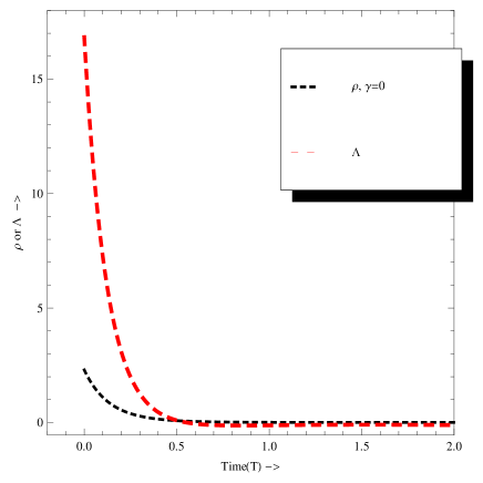
Figure 1: The plot of energy density $\rho$ and cosmological constant $\Lambda$ Vs. time $T$ for $\gamma=0$. Here $k_{1}=3.1$, $k_{4}=1.0$.

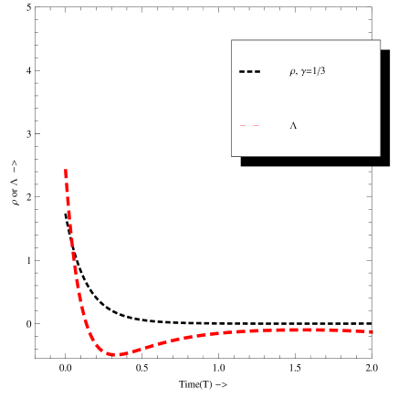
Figure 2: The plot of energy density $\rho$ and cosmological constant $\Lambda$ Vs. time $T$ for $\gamma=\frac{1}{3}$. Here $k_{1}=3.1$, $k_{4}=1.0$.

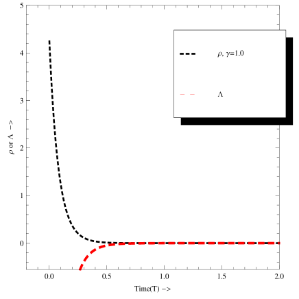
Figure 3: The plot of energy density $\rho$ and cosmological constant $\Lambda$ Vs. time $T$ for $\gamma=1$. Here $k_{1}=3.1$, $k_{4}=1.0$.

For the specification of $\Lambda(T)$, we assume that the fluid obeys an equation of state of the form

$$p=\gamma\rho,$$ (38)

where $\gamma(0\leq\gamma\leq 1)$ is a constant. Using (38) in (36) and (37), we obtain

$$8\pi(1+\gamma)\rho=\frac{6}{k_{4}^{2}}(k_{1}-2T)^{2}\exp{\left[2T(T-k_{1})\right]}.$$ (39)

Eliminating $\rho$ between Eqs. (37) and (39), we obtain

$$(1+\gamma)\Lambda=-\frac{12(1+\gamma)}{k_{4}^{2}}\exp{[2T(T-k_{1})]}+\frac{3(1-\gamma)}{k_{4}^{2}}(k_{1}-2T)^{2}\exp{\left[2T(T-k_{1})\right]}.$$ (40)

Using above solutions, it can be easily seen that the energy conservation equation (11) in perfect fluid distribution is satisfied.

From Eq. (39), we observe that $\rho(t)$ is a decreasing function of time and $\rho>0$ always for $\gamma=0,\frac{1}{3},1$. Figures $1,2,3$ (${\rho}~{}{\rm and}~{}{\Lambda}$ are in geometrical units in entire paper) show this behaviour of energy density for vacuum ($\gamma=0$), radiating ($\gamma=\frac{1}{3}$) and Zeldovice ($\gamma=1$) universes. From Eq. (40), we note that the cosmological term $\Lambda$ is a decreasing function of time. From Figure 1 we observe that $\Lambda$, for empty universe, is a positive decreasing function of time and and it approaches to a positive small value at late time. Recent cosmological observations (Perlmutter et al. [32]$-$[34] and Riess et al. [35, 36], Garnavich et al. [37, 38], Schmidt et al. [39]) suggest the existence of a positive cosmological constant $\Lambda$ with the magnitude $\Lambda(G\hbar/c^{3})\approx 10^{-123}$. These observations on magnitude and red-shift of type Ia supernova suggest that our universe may be an accelerating one with induced cosmological density through the cosmological $\Lambda$-term.

From Figure $2$, we observe that the $\Lambda$, in radiating universe, decreases sharply with time and goes to a negative point and then increases with time approaching to a constant value near zero. This is to be taken as a representative case of physical viability of the model. From Figure 3, it is also observed that for Zeldovice universe ($\gamma=1$), $\Lambda$ is negative at initial stage but it increases very rapidly with time and ultimately approaches to a positive constant near zero. Thus $\Lambda$ makes a transition from negative to positive value near zero at the present epoch.

The behaviour of the universe in the above models are to be determined by the cosmological term $\Lambda$, this term has the same effect as a uniform mass density $\rho_{eff}=-\Lambda/4\pi$ which is constant time. A positive value of $\Lambda$ corresponds to a negative effective mass density (repulsion). Hence, we expect that in the universe with a positive value of $\Lambda$ the expansion will tend to accelerate whereas in the universe with negative value of $\Lambda$ the expansion will slow down, stop and reverse. In a universe with both matter and vacuum energy, there is a competition between the tendency of $\Lambda$ to cause acceleration and the tendency of matter to cause deceleration with the ultimate fate of the universe depending on the precise amounts of each component. This continues to be true in the presence of spatial curvature, and with a nonzero cosmological constant it is no longer true that the negatively curved (“open”) universes expand indefinitely while positively curved (“closed”) universes will necessarily re-collapse - each of the four combinations of negative or positive curvature and eternal expansion or eventual re-collapse become possible for appropriate values of the parameters. There may even be a delicate balance, in which the competition between matter and vacuum energy is needed drawn and the universe is static (non expanding). The search for such a solution was Einstein’s original motivation for introducing the cosmological constant.

Some Physical and Geometric Features of the Model
The expressions for kinematics parameters i. e. the scalar of expansion $\theta$, shear scalar $\sigma$, average scale factor $S$, proper volume $V^{3}$ and average anisotropy parameter $A_{p}$ for the model (35) are given by

$$\theta=\frac{1}{k_{4}}\left[6+(k_{1}-2T)^{2}\right]\exp{[T(T-k_{1})]},$$ (41)

$$\sigma=\frac{1}{k_{4}\sqrt{3}}(k_{1}-2T)^{2}\exp{[T(T-k_{1})]},$$ (42)

$$S=\frac{k_{4}^{\frac{2}{3}}}{k_{3}^{\frac{1}{3}}(k_{1}-2T)\exp{[\frac{T(T-k_{1})}{3}}]}.$$ (43)

$$V^{3}=\sqrt{-g}=\frac{k_{4}^{4}\exp{[-2T(T-k_{1})]}}{k_{3}^{2}(k_{1}-2T)^{4}},$$ (44)

$$A_{p}=\frac{4}{3}.$$ (45)

The directional Hubble’s parameters $H_{x}$, $H_{y}$ and $H_{z}$ are given by

$$H_{x}=\frac{1}{k_{4}}[(k_{1}-2T)^{2}+2]\exp{[T(T-k_{1}}],$$ (46)

$$H_{y}=H_{z}=\frac{2}{k_{4}}\exp{[T(T-k_{1}}],$$ (47)

where the mean Hubble’s parameter is given by

$$H=\frac{1}{3k_{4}}\{6+(k_{1}-2T)^{2}\}\exp{[T(T-k_{1})]}$$ (48)

Figure 4: The plot of average scale factor $S$ Vs. time. Here $k_{1}=18$, $k_{3}=1.0$, $k_{4}=1.0$.

The model (35) starts expansion with a big-bang singularity from $T=-\infty$ and it goes on expanding till $T=\frac{k_{1}-{1}}{2}$ respectively correspond to the cosmic time $t=0$ and $t=\infty$. The is found to be realistic everywhere in this time interval for $\Lambda>-\frac{12}{k_{4}^{2}}\exp{\left(-\frac{k_{1}^{2}}{2}\right)}$. The model behaves like a steady-state de-Sitter type universe at late times where the physical and kinematic parameters $\rho$, $p$, $\theta$ tend to a finite value, however shear vanishes there. The model has a point type singularity at time $T=k_{1}$. The singular behaviour may be close to cosmic origin or outside the evolution. The average anisotropy parameter $A_{p}$ remains uniform and isotropic through out the evolution of the universe. This would depend on physical properties of matter and radiation. This may need detailed study to make better quantifiable view. From Figure $4$, it can be seen that in the early stages of the universe, i. e., $t=0$, the scale factor of the universe had been approximately constant and had increased very slowly. At specific time the universe had exploded suddenly and expanded to large scale. This is good matching with big bang scenario. This is indicated in first part (top) of Figure $4$. Later singular behaviour depends on $(k_{1},T)$.

3.2 Solutions For Bulk Viscous Fluid

Astronomical observations of large-scale distribution of galaxies of our universe show that the distribution of matter can be satisfactorily described by a perfect fluid. But large entropy per baryon and the remarkable degree of isotropy of the cosmic microwave background radiation, suggest that we should analyze dissipative effects in cosmology. Further, there are several processes which are expected to give rise to viscous effect. These are the decoupling of neutrinos during the radiation era and the recombination era [50], decay of massive super string modes into massless modes [51], gravitational string production [52, 53] and particle creation effect in grand unification era [54]. It is known that the introduction of bulk viscosity can avoid the big bang singularity. Thus, we should consider the presence of a material distribution other than a perfect fluid to have realistic cosmological models (see Grøn [55] for a review on cosmological models with bulk viscosity). A uniform cosmological model filled with fluid which possesses pressure and second (bulk) viscosity was developed by Murphy [56]. The solutions that he found exhibit an interesting feature that the big bang type singularity appears in the infinite past.

In presence of bulk viscous fluid distribution, we replace isotropic pressure $p$ by effective pressure $\bar{p}$ in Eq. (36) where

$$\bar{p}=p-\xi v^{i}_{;i},$$ (49)

where $\xi$ is the coefficient of bulk viscosity.
The expression for effective pressure $\bar{p}$ for the model Eq. (35) is given by

$$8\pi\bar{p}=8\pi(p-\xi v^{i}_{;i})=-\frac{3}{k_{4}^{2}}\left[4-(k_{1}-2T)^{2}\right]\exp{[2T(T-k_{1})]}-\Lambda(T).$$ (50)

Thus, for given $\xi(t)$ we can solve for the cosmological parameters. In most of the investigation involving bulk viscosity is assumed to be a simple power function of the energy density (Pavon [57], Maartens [58], Zimdahl [59], Santos [60])

$$\xi(t)=\xi_{0}\rho^{n},$$ (51)

where $\xi_{0}$ and $n$ are constants. For small density, $n$ may even be equal to unity as used in Murphy’s work [56] for simplicity. If $n=1$, Eq. (51) may correspond to a radiative fluid (Weinberg [11]). Near the big bang, $0\leq n\leq\frac{1}{2}$ is a more appropriate assumption (Belinskii and Khalatnikov [61]) to obtain realistic models.

For simplicity sake and for realistic models of physical importance, we consider the following two cases ($n=0,1$):

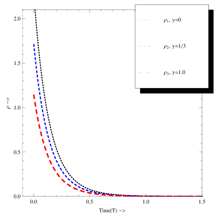
Figure 5: The plot of energy density $\rho$ Vs. time $T$ for $\gamma=0,\frac{1}{3},1$. Here $k_{1}=4.5$, $k_{4}=1.00$, $\xi_{0}=1.00$, $n=0$.

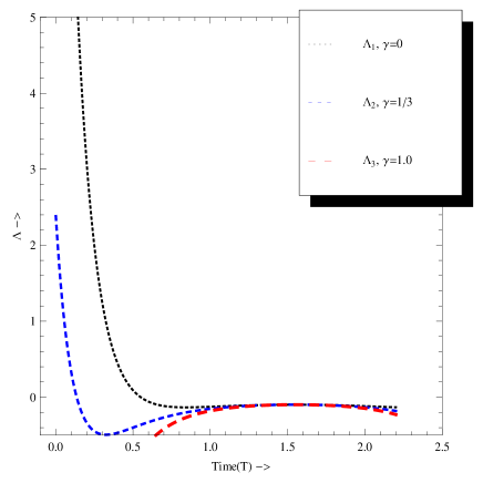
Figure 6: The plot of cosmological constant $\Lambda$ Vs. time $T$ for $\gamma=0,\frac{1}{3},1$. Here $k_{1}=4.5$, $k_{4}=1.00$, $\xi_{0}=1.00$, $n=0$.

3.2.1 Model I: When $n=0$

When $n=0$, Eq. (51) reduces to $\xi=\xi_{0}=$ constant. With the use of Eqs. (37), (38) and (41), Eq. (50) reduces to

$$8\pi(1+\gamma)\rho=\frac{6}{k_{4}^{2}}(k_{1}-2T)^{2}\exp{[2T(T-k_{1})]}+$$

$$\frac{8\pi\xi_{0}}{k_{4}}\{6+(k_{1}-2T)^{2}\}\exp{[2T(T-k_{1})]}.$$ (52)

Eliminating $\rho(t)$ between Eqs. (37) and (52), we obtain

$$(1+\gamma)\Lambda=-\frac{12(1+\gamma)}{k_{4}^{2}}\exp{[2T(T-k_{1})]}+\frac{3(1-\gamma)}{k_{4}^{2}}(k_{1}-2T)^{2}\exp{[2T(T-k_{1})]}$$

$$+\frac{8\pi\xi_{0}}{k_{4}}\{6+(k_{1}-2T)^{2}\}\exp{[T(T-k_{1})]}.$$ (53)

3.2.2 Model II: When $n=1$

When $n=1$, Eq. (51) reduces to $\xi=\xi_{0}\rho$. With the use of Eqs. (37), (38) and (41), Eq. (50) reduces to

$$\rho=\frac{3(k_{1}-2T)^{2}\exp{[2T(T-k_{1})]}}{4\pi k_{4}\left[k_{4}(1+\gamma)-\xi_{0}\{6+(k_{1}-2T)^{2}\}\exp{[T(T-k_{1})]}\right]}.$$ (54)

Eliminating $\rho(t)$ between Eqs. (37) and (54), we obtain

$$\Lambda=-\frac{12}{k_{4}^{2}}\exp{[2T(T-k_{1})]}-\frac{3(k_{1}-2T)^{2}\exp{[2T(T-k_{1})]}}{k_{4}^{2}\Bigl{[}k_{4}(\gamma+1)-\xi_{0}\{6+(k_{1}-2T)^{2}\}\exp{[T(T-k_{1})]}\Bigr{]}}\times$$

$$\Bigl{[}k_{4}(\gamma-1)-\xi_{0}\{6+(k_{1}-2T)^{2}\}\exp{[T(T-k_{1})]}\Bigr{]}.$$ (55)

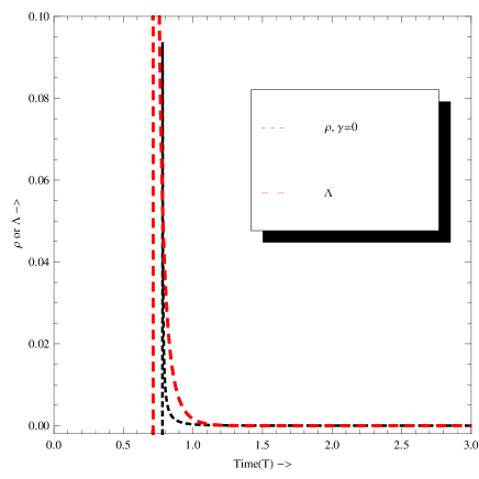
Figure 7: The plot of energy density $\rho$ and cosmological term $\Lambda$ Vs. time $T$ for $\gamma=0$. Here $k_{1}=5.5$, $k_{4}=1.00$, $\xi_{0}=1.00$, $n=1$.

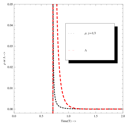
Figure 8: The plot of energy density $\rho$ and cosmological term $\Lambda$ Vs. time $T$ for $\gamma=\frac{1}{3}$. Here $k_{1}=5.5$, $k_{4}=1.00$, $\xi_{0}=1.00$, $n=0$.

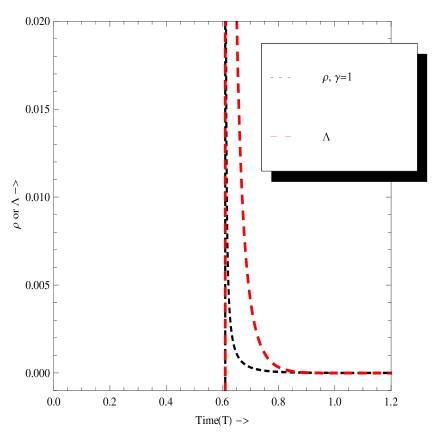
Figure 9: The plot of energy density $\rho$ and cosmological term $\Lambda$ Vs. time $T$ for $\gamma=1$. Here $k_{1}=5.5$, $k_{4}=1.00$, $\xi_{0}=1.00$, $n=0$.

In the case of bulk viscous fluid, the energy conservation equation $T^{ij}_{;j}=0$, leads to the following expression

$$\dot{\Lambda}+\dot{\rho}+(\rho+\bar{p})\left(\frac{\dot{A}}{A}+2\frac{\dot{B}}{B}\right)=0.$$ (56)

It is worth mentioned here that above solutions for bulk viscous fluid also satisfy the energy conservation equation (56).

From Eqs. (52), we observe that energy density $\rho$ for the case $n=0$, is a positive decreasing function of time for $\gamma=0,\frac{1}{3},1$. Figure $5$ depicts the variation of the energy density $\rho$ versus time $T$ for $\gamma=0,\frac{1}{3},1$ for Model I ($n=0$). The figure shows the positive decreasing function of energy density and which becomes zero at present epoch as anticipated.

From Eqs. (53), we observe that cosmological constant $\Lambda$ for the case $n=0$, is a decreasing function of time for $\gamma=0,\frac{1}{3}$. Figure $6$ plots the variation of $\Lambda$ versus $T$ for $\gamma=0,\frac{1}{3},1$. Here we observe that cosmological term $\Lambda$, for vacuum and radiating universe, is a decreasing function of time whereas for Zeldovice universe it is negative and increasing function of time. We also observe that in all these three universes the $\Lambda$-term approaches to the same small negative value almost closer to zero at late time. Models with negative cosmological constant have been investigated by Yadav [62], Saha and Boyadjiev [63], Pedram et al. [64], Biswas and Mazumdar [65], Jotania et al . [66]. Really at present the estimation of $\Lambda$ is not only complicated but it is uncertain and indirect too. However, the Einstein-Maxwell theory indicates to a different approach which looks simpler and more significant, since a possibility is illustrated for $\Lambda\leq 0$ i.e. for the case when the presence of $\Lambda$ decelerates the expansion of the universe.

From Eqs. (54) and (55), we observe that energy density $\rho$ and cosmological constant $\Lambda$, for the case ($n=1$) are a decreasing function of time and both are small positive at late time for vacuum, radiating and Zeldovice universes. Figures $7$, $8$ and $9$ depict the energy density ($\rho$) and $\Lambda$-term versus time $T$ for empty, radiating and Zeldovice universe respectively. The nature of $\rho$ and $\Lambda$ can be seen in these figures.

The effect of bulk viscosity is to produce a change in perfect fluid and therefore exhibits essential influence on the character of the solution. A comparative inspection of Figures show apparent evolution of time due to perfect fluid and bulk viscous fluid. It is apparent that the vacuum energy density ($\rho$) decays much fast in later case. It also shows the effect of uniform viscosity model and linear viscosity model. Even in these cases, the decay of vacuum energy density is much faster than uniform. So, the coupling parameter ${{\xi}_{0}}$ would be related with physical structure of the matter and provides mechanism to incorporate relevant property. In order to say more specific, detailed study would be needed which would be reported in future. Similar behaviour is observed for the cosmological constant $\Lambda$. We also observe here that Murphy’s [56] conclusion about the absence of a big bang type singularity in the infinite past in models with bulk viscous fluid in general, is not true. The results obtained by Myung and Cho [67] also show that, it is not generally valid since for some cases big bang singularity occurs in finite past. For both models, it is observed that the effect of viscosity prevents the shear and the free gravitational field from withering away.

4 Solution of Field Equations for Second Case

In this case there is a ‘gravitational wrench’ of unit ‘pitch’ in the free gravitational field i.e. $E_{\alpha\beta}=\pm H_{\alpha\beta}$. Therefore we have

$$E_{\alpha\beta}=\kappa H_{\alpha\beta},~{}~{}~{}~{}\mbox{$\kappa^{2}=1$}.$$ (57)

In this case, Bali et al. [49] have investigated the solution given by

$$ds^{2}=\frac{(2\tau^{2}+3\kappa\tau+2)^{\frac{1}{2}}}{\tau^{2}}\exp{\left(\frac{3\kappa}{\sqrt{7}}\tan^{-1}{\frac{(4\tau+3\kappa)}{\sqrt{7}}}\right)}\Biggl{[}-\frac{d\tau^{2}}{(2\tau^{2}+3\kappa\tau+2)6{2}}$$

$$+dx^{2}+(2\tau^{2}+3\kappa\tau+2)^{\frac{1}{2}}\exp{\left(-\frac{3\kappa}{\sqrt{7}}\tan^{-1}{\frac{(4\tau+3\kappa)}{\sqrt{7}}}\right)}\{e^{2x}dy^{2}+e^{-2x}dz^{2}\}\Biggr{]}.$$ (58)

The expressions for pressure $p$ and energy density $\rho$ for the model (58) are obtained as

$$8\pi p=\frac{(12\kappa\tau^{3}+29\tau^{2}+72\kappa\tau-48)}{4(2\tau^{2}+3\kappa\tau+2)^{\frac{1}{2}}}\exp{\left(-\frac{3\kappa}{\sqrt{7}}\tan^{-1}{\frac{(4\tau+3\kappa)}{\sqrt{7}}}\right)}-\Lambda(\tau)$$ (59)

$$8\pi\rho=\frac{(12\kappa\tau^{3}+39\tau^{2}+72\kappa\tau+48)}{4(2\tau^{2}+3\kappa\tau+2)^{\frac{1}{2}}}\exp{\left(-\frac{3\kappa}{\sqrt{7}}\tan^{-1}{\frac{(4\tau+3\kappa)}{\sqrt{7}}}\right)}+\Lambda(\tau)$$ (60)

For the specification of $\Lambda(\tau)$, we assume that the fluid obeys an equation of state of the form (38). Using Eqs. (38) in (59) and (60), we obtain

$$8\pi(1+\gamma)\rho=\left[\frac{6\kappa\tau^{3}+17\tau^{2}+36\kappa\tau}{(2\tau^{2}+3\kappa\tau+2)^{\frac{1}{2}}}\right]\exp{\left\{-\frac{3\kappa}{\sqrt{7}}\tan^{-1}{\left(\frac{4\tau+3\kappa}{\sqrt{7}}\right)}\right\}}.$$ (61)

Eliminating $\rho$ between (59) and (61), we obtain

$$\Lambda=-\left[\frac{12(\gamma-1)\kappa(\tau^{2}+6)\tau+T^{2}(39\gamma-29)+48(\gamma+1)}{4(\gamma+1)(2T^{2}+3\kappa T+2)^{\frac{1}{2}}}\right]\times$$

$$\exp{\left\{-\frac{3\kappa}{\sqrt{7}}\tan^{-1}{\left(\frac{4T+3\kappa}{\sqrt{7}}\right)}\right\}}$$ (62)

From preliminary study, we find that both energy density and cosmological constant are negative. Hence it will not be studied. It also shows singular behaviour in energy density at later stage of the evolution. Hence, the model is unphysical for further study.

5 Discussion and Concluding Remarks

In this paper, we have studied properties of the free gravitational field and their invariant characterizations and obtained LRS Bianchi type ${\rm VI}_{0}$ cosmological models imposing different conditions on the free gravitational field. In first case, where fee gravitational field is purely magnetic type, we observe that the energy density${\rho}$ and cosmological constant ${\Lambda}$ are well behaved. Also the effect of bulk viscous fluid distribution in the universe is compared with perfect fluid model. We observe that due to presence of bulk viscous fluid, the rate of decrease in energy density is faster compared to perfect fluid model. The linear relation of the coefficient of bulk viscosity with mass density provides further enhance decrease rate (see figures). Since we had considered extension of the various models, detailed physical parameter study would be reported in future. Important incorporation is time-dependence of cosmological constant ${\Lambda}$. The similar enhance decrease rate is also observed for ${\Lambda}$ (see figures). The scale factor dependence is also reported. Recent observational data [68]$-$[70] reveal the presence of a non-vanishing positive cosmological term $\Lambda$ as we have found in our present theoretical study.

References

- [1] L. M. Krauss and M. S. Turner, Gen. Rel. Gravit. 27, 1137 (1995).
- [2] S. L. Adler, Rev. Mod. Phys. 54, 729 (1982).
- [3] S. Weinberg, Phys. Rev. Lett. 19, 1264 (1967).
- [4] A. D. Linde, Sov. Phys. Lett. 19, 183 (1974).
- [5] J. M. Overduin and F. I. Cooperstock, Phys. Rev. D 58, 043506 (1998).
- [6] J. M. Overduin, Ap. J. 517, L1 (1999).
- [7] J. M. Overduin, Phys. Rev. D 62, 102001 (2000).
- [8] H. Liu and P. S. Wesson, Astrophys. J. 562, 1 (2001).
- [9] S. Podariu and B. Ratra, Astrophys. J. 532, 109 (2000).
- [10] K. Croswell, New Scientist April 18 (1994).
- [11] S. Weinberge, Gravitation and Cosmology, Wiley, New York (1972).
- [12] S. M. Caroll, W. H. Press and E. L. Turner, Ann. Rev. Astron. Astrophys. 30, 499 (1992).
- [13] P. J. E. Peebles, Rev. Mod. Phys. 75, 559 (2003).
- [14] V. Sahani and A. Starobinsky, Int. J. Mod. Phys. D 9, 373 (2000).
- [15] T. Padmanabhan, Phys. Rep. 380, 235 (2003).
- [16] T. Padmanabhan, Gen. Rel. Grav. 40, 529 (2008).
- [17] C. P. Singh, S. Kumar and A. Pradhan, Class. Quantum Grav. 24, 455 (2007).
- [18] A. Pradhan and O. P. Pandey, Int. J. Mod. Phys. D 12, 1299 (2003).
- [19] A. Pradhan and P. Pandey, Astrophys. Space Sci. 301, 221 (2006).
- [20] A. Pradhan and S. Singh, Int. J. Mod. Phys. D 13, 503 (2004).
- [21] A. Pradhan, A. K. Singh and S. Otarod, Roman. J. Phys. 52, 415 (2007).
- [22] A. Pradhan, K. Jotania and A. Singh, Braz. J. Phys. 38, 167 (2008).
- [23] A. Pradhan, Fizika B (Zagreb) 16, 205 (2007).
- [24] A. Pradhan, Commun. Theor. Phys. 51, 367 (2009).
- [25] A. Pradhan and A. Kumar, Int. J. Mod. Phys. D 10, 291 (2001).
- [26] A. Pradhan and V. K. Yadav, Int. J. Mod Phys. D 11, 983 (2002).
- [27] A. Pradhan and H. R. Pandey, Int. J. Mod. Phys. D 12, 941 (2003).
- [28] A. Pradhan and P. Pandey, Czech. J. Phys. 55, 749 (2005).
- [29] Abdussattar and R. G. Vishwakarma, Pramana - J. Phys. 47, 41 (1996).
- [30] S. Kalita, H. L. Duorah and K. Duorah, Ind. J. Phys. 84, 629 (2010).
- [31] A. Pradhan and K. Jotania, Ind. J. Phys. 85, 497 (2011).
- [32] S. Perlmutter et al., Astrophys. J. 483, 565 (1997).
- [33] S. Perlmutter et al., Nature 391, 51 (1998).
- [34] S. Perlmutter et al., Astrophys. J. 517, 565 (1999).
- [35] A. G. Riess et al., Astron. J. 116, 1009 (1998).
- [36] A. G. Riess et al., Astrophys. J. 607, 665 (2004).
- [37] P. M. Garnavich et al., Astrophys. J. 493, L53 (1998).
- [38] P. M. Garnavich et al., Astrophys. J. 509, 74 (1998).
- [39] B. P. Schmidt et al., Astrophys. J. 507, 46 (1998).
- [40] G. F. R. Ellis, General Relativity and Cosmology, ed. R. K. Sachs, New York: Academic Press (1971).
- [41] S. R. Roy and S. K. Banerjee, Astrophys. Space Sci. 167, 81 (1990).
- [42] L. Bianchi, Lezioni Sull a Teoria Deigruppi Continui di Transformazioni Pisa, Editiozi Speern (1918).
- [43] J. D. Barrow, Mon. Not. R. Astron. Soc. 211, 221 (1984).
- [44] S. R. Roy and J. P. Singh, Acta Physica Austriaca 55, 57 (1983).
- [45] R. Tikekar and L. K. Patel, Pramana - J. Phys. 42, 483 (1994).
- [46] R. Bali, R. Banerjee and S. K. Banerjee, Astrophys. Space Sci. 317, 21 (2008).
- [47] R. Bali, A. Pradhan and A. Hassan, Int. J. Theor. Phys. 47, 2594 (2008).
- [48] A. Pradhan and R. Bali, EJTP 19, 91 (2008).
- [49] R. Bali, R. Banerjee and S. K. Banerjee, EJTP 21, 165 (2009).
- [50] E. W. Kolb and M. S. Turner, The Early Universe, Addison - Wesley, U S A (1990).
- [51] S. Myung and B. M. Cho, Mod. Phys. Lett. A 1, 37 (1986).
- [52] N. Turok, Phys. Rev. Lett. 60, 549 (1988).
- [53] J. D. Barrow, Nucl. Phys. B 310, 243 (1988).
- [54] C. Wolf, S.-Afr. Tydskr. 14, 68 (1991).
- [55] Ø. Grøn, Astrophys. Space Sci. 173, 191 (1990).
- [56] G. L. Murphy, Phys. Rev. D 8, 4231 (1973).
- [57] D. Pavon, J. Bafaluy and D. Jou, Class. Quant. Grav. 8, 357 (1996).
- [58] R. Maartens, Class Quantum Gravit. 12, 1455 (1995).
- [59] W. Zimdahl, Phys. Rev. D 53, 5483 (1996).
- [60] N. O. Santos, R. S. Dias and A. Banerjee, J. Math. Phys. 26, 878 (1985).
- [61] U. A. Belinskii and I. M. Khalatnikov, Sov. Phys. JETP 42, 205 (1976).
- [62] A. K. Yadav, arXiv:0911.0177.
- [63] B. Saha, T. Boyadjiev, Phys. Rev. D 69, 124010 (2004).
- [64] P. Pedram, M. Mirzaei, S. Jalalzadeh, S. S. Gousheh, Gen. Rel. Grav. 40, 1663 (2008).
- [65] T. Biswas, A. Mazumdar, Phys. Rev. D 80, 023519 (2009).
- [66] K. Jotania, P. Yadav, S. A. Faruqi, Int. J. Theor. Phys. 50, 1424 (2011).
- [67] S. Myung, B. M. Cho, Mod. Phys. Lett. A 1, 37 (1986).
- [68] BOOMERanG (P. de Bernardis et al.), Nature 404, 955 (2000).
- [69] MAXIMA (S. Hanany et al.), Astrophys. J. Lett. 545, 5 (2000).
- [70] D. N. Sperger, Astrophys. J. Suppl. 148, 175 (2003).