The Parkes Galactic Meridian Survey (PGMS): observations and CMB polarization foreground analysis

Abstract

We present observations and CMB foreground analysis of the Parkes Galactic Meridian Survey (PGMS), an investigation of the Galactic latitude behaviour of the polarized synchrotron emission at 2.3 GHz with the Parkes Radio Telescope. The survey consists of a $5\degr$ wide strip along the Galactic meridian $l=254\degr$ extending from Galactic plane to South Galactic pole. We identify three zones distinguished by polarized emission properties: the disc, the halo, and a transition region connecting them. The halo section lies at latitudes $|b|>40\degr$ and has weak and smooth polarized emission mostly at large scale with steep angular power spectra of median slope $\beta_{\rm med}\sim-2.6$. The disc region covers the latitudes $|b|<20\degr$ and has a brighter, more complex emission dominated by the small scales with flatter spectra of median slope $\beta_{\rm med}=-1.8$. The transition region has steep spectra as in the halo, but the emission increases toward the Galactic plane from halo to disc levels. The change of slope and emission structure at $b\sim-20\degr$ is sudden, indicating a sharp disc-halo transition. The whole halo section is just one environment extended over $50\degr$ with very low emission which, once scaled to 70 GHz, is equivalent to the CMB $B$–Mode emission for a tensor–to–scalar perturbation power ratio $r_{\rm halo}=(3.3\pm 0.4)\times 10^{-3}$. Applying a conservative cleaning procedure, we estimate an $r$ detection limit of $\delta r\sim 2\times 10^{-3}$ at 70 GHz (3-sigma C.L.) and, assuming a dust polariztion fraction $<$ 12%, $\delta r\sim 1\times 10^{-2}$ at 150 GHz. The 150 GHz limit matches the goals of planned sub-orbital experiments, which can therefore be conducted at this high frequency. The 70 GHz limit is close to the goal of proposed next generation space missions, which thus might not strictly require space-based platforms.

1 Introduction

The study of the Galactic polarized synchrotron emission is essential for two cutting-edge fields of current astrophysics research: the detection of the $B$–Mode of the Cosmic Microwave Background (CMB), for which the Galactic synchrotron is foreground emission, and the investigation of the magnetic field of the Galaxy.

The CMB $B$–mode is a direct signature of the primordial gravitational wave background (GWB) left by inflation (e.g., Kamionkowski & Kosowsky 1998; Boyle, Steinhardt, & Turok 2006). The amplitude of its angular power spectrum is proportional to the GWB power, which is conveniently expressed relative to the amplitude of density fluctuations—the so-called “tensor-to-scalar perturbation power ratio” $r$. Still undetected, the current upper limit is set to $r<0.20$ (95% C.L., Komatsu et al. 2009) by the results of the Wilkinson Microwave Anisotropy Probe (WMAP). A detection of the $B$–Mode would be evidence for primordial gravitational waves, and a measurement of $r$ would help distinguish among several inflation models and investigate the physics of the early stages of the Universe.

Reaching this spectacular science goal will be difficult because of the tiny size of the CMB $B$-Mode signal, fainter than the current upper limit of 0.1 $\mu$K, and perhaps as faint as the 1 nK corresponding to the smallest $r$ accessible by CMB ($r\sim 10^{-5}$, Amarie, Hirata & Seljak 2005). At such low levels the cosmic signal is easily obscured by the Galactic foreground of the synchrotron and dust emissions.

Investigations of the synchrotron contribution have been conducted over recent years, but data are still insufficient to give a comprehensive view (Fig. 1). Page et al. (2007) analysed the 23 GHz WMAP polarized maps and find that the typical emission at high Galactic latitude is strong: at 70 GHz it is equivalent to $r\sim 0.3$, even higher than the current upper limit. An analysis of the same WMAP data by Carretti et al. (2006b) identified regions covering about 15 per cent of the sky with much lower emission levels, offering a better chance for $B$–Mode detection. In these regions the polarized foreground is fainter, equivalent to a $B$–Mode signal corresponding to $r$ in the range $[1\times 10^{-3},1\times 10^{-2}]$. A better characerization of the polarized foreground is crucial especially for sub-orbital experiments (ground-based and balloon-borne), which will observe small sky areas.

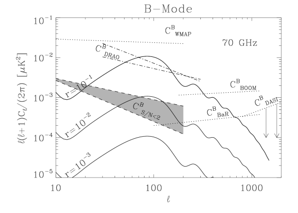
Figure 1: Summary of the current knowledge of the $B$–Mode power spectra of the Galactic synchrotron emission. Spectra are estimated at 70 GHz. A brightness temperature frequency spectral index of $\alpha=-3.1$ has been assumed for all extrapolations. $C^{B}_{\rm WMAP}$ is the general contamination at high Galactic latitude, as estimated by the WMAP team using a $\sim 75\%$ sky fraction at 22.8-GHz (Page et al., 2007). Spectra measured in small areas selected for their low emission are also shown: the target fields of the experiments BOOMERanG ($C^{B}_{\rm BOOM}$, Carretti et al. 2005b) and BaR-SPOrt ($C^{B}_{\rm BaR}$, Carretti et al. 2006a), and the upper limit found in the two fields of the experiment DASI ($C^{B}_{\rm DASI}$, Bernardi et al. 2006). Finally, $C_{S/N<2}$ shows the estimate of the emission in the best 15% of the sky (Carretti et al. 2006b, the shaded area indicates the uncertainties), while $C_{\rm DRAO}$ the values found in some intermediate regions using 1.4 GHz data (La Porta et al., 2006). For comparison, CMB spectra for three values of $r$ are also shown.

The design of future experiments is dependent on the frequency of minimum foreground emission. WMAP finds that this is in the range 60–70 GHz for high Galactic latitudes (Page et al., 2007), but it remains unknown for the lowest emission part of the sky. It has been suggested that the dust emission might have deeper minima than the synchrotron in the areas of lowest emission (e.g., Lange 2008), shifting the best window for $B$–Mode detection to higher frequencies.

Synchrotron emission from the Milky Way is not only a foreground for CMB polarization measurements, but can also be used to study the Galactic magnetic field. The total intensity of synchrotron emission can be used to estimate the total magnetic field strength, while the polarized intensity gives the strength of the regular component. This analysis in external galaxies has shown that the spiral arms are usually dominated by a small-scale, tangled, magnetic field with a weaker coherent large-scale field aligned with the arms. In the inter-arm regions the regular component dominates and in some spirals, magnetic arms with coherent scales up to the size of the disc have been detected in between the gas arms (e.g. see Beck 2008 for a review).

The synchrotron emissivity of our own Galaxy is harder to understand because of our location inside it, but has the advantage that it can be studied in detail. Frequency dependent synchrotron depolarization can be used to determine typical scale and strength of small-scale magnetic fields (e.g.Gaensler et al. 2001), and all-sky synchrotron emissivity maps can characterise the synchrotron scale height (Beuermann et al., 1985), or can be used for large-scale modeling of the Galactic magnetic field, especially in the halo. The relative parity of the toroidal magnetic field component is still under discussion (see e.g., Han 1997; Frick et al. 2001; Sun et al. 2008). Jansson et al. (2009) use WMAP synchrotron maps at 23 GHz to show that the magnetic field behaviour in the Galactic disc and halo may differ considerably.

Data from external galaxies does not help in constraining the Milky Way magnetic halo, as there is a wide variety of magnetic field configurations: from galaxies without evident halo field, to X-shaped fields centred at the galaxy centre, to large almost spherical magnetic halos (see Beck 2008 for a review).

Recent maps of polarized Galactic synchrotron radiation at 1.4 and 22.8 GHz (Wolleben et al., 2006; Testori et al., 2008; Page et al., 2007) show polarized emission across the entire sky, and can be used to study the Galactic magnetic field. However, the 1.4 GHz maps show that the disc emission is strongly depolarized up to latitudes $|b|\approx 30^{\circ}$ (Wolleben et al., 2006; Testori et al., 2008), while Faraday depolarization effects are still present up to $|b|\approx 40-50^{\circ}$ (Carretti et al., 2005a). Furthermore, those data consist of a single frequency band and do not enable rotation measure computations. The WMAP data at 22.8 GHz are virtually unaffected by Faraday rotation (FR) effects, but the sensitivity is not sufficient since, once binned in $2\degr$ pixels, about 55% of the sky has a signal to noise ratio $S/N<3$. This area corresponds to all the high Galactic latitudes with the exception of large local structures, which is most of the sky useful both for CMB studies and to investigate the Galactic magnetic field.

Therefore, synchrotron maps at intermediate frequencies over all Galactic latitudes are needed to explore the behaviour of the contamination of the CMB with latitude as well as to study the Galactic magnetic field in the disc, the halo, and the disc-halo transition.

In this work we present the Parkes Galactic Meridian Survey (PGMS), a survey conducted with the Parkes Radio Telescope to cover a strip along an entire southern Galactic meridian at 2.3 GHz. The area is free from large local structures, making it ideal for investigating both the CMB foregrounds and the Galactic magnetic field. The PGMS overlaps the target area of several CMB experiments like BOOMERanG (Masi et al., 2006), QUaD (Brown et al., 2009), BICEP (Chiang et al., 2009), and EBEX (Grainger et al., 2008). Our results may have direct implications for all these experiments.

In this paper we present the survey, observations, and a characterisation of the polarized emission. We also present an analysis of the measured emission as a contaminating foreground to CMB $B$–mode studies. Analysis and implications for the Galactic magnetic field will be subject of a forthcoming paper (Paper II, Haverkorn et al. 2010 in preparation). A third paper will deal with the polarized extragalactic sources (paper III, Bernardi et al. 2010 in preparation).

Survey and observations are presented in Section 2, the ground emission analysis in Section 3, and the maps in Section 4. The analysis of both the angular power spectrum and emission behaviour is presented in Section 5, while the dust contribution is investigated in Section 6. The detection limits of $r$ are discussed in Section 7 and, finally, our summary and conclusions are reported in Section 8.

2 The Parkes Galactic Meridian Survey

The available data and the properties of the synchrotron emission discussed in Section 1 lead to the following main requirements for a survey. Observations must

1. be conducted at a low enough radio frequency for the synchrotron emission to dominate the other diffuse emission components, but at a frequency higher than 1.4 GHz to avoid significant Faraday Rotation effects;

2. cover all latitudes from the Galactic plane to the pole, to explore the behaviour with the Galactic latitude $b$;

3. cover regions free from large local structures, such as the big radio loops, that would distort the estimates of typical conditions at high latitudes.

The Parkes Galactic Meridian Survey (PGMS) is a project to survey the diffuse polarized emission along a Galactic meridian designed to satisfy these requirements. It surveys a $5\degr\times 90\degr$ strip along the entire southern meridian $l=254^{\circ}$ from the Galactic plane to the south Galactic pole (Fig. 2). The observations have been made at 2.3 GHz with the Parkes Radio Telescope (NSW, Australia), a facility operated by the ATNF - CSIRO Astronomy and Space Science a division of CSIRO. It also includes an $10\degr\times 10\degr$ extension centred at $l=251^{\circ}$ and $b=-35^{\circ}$.

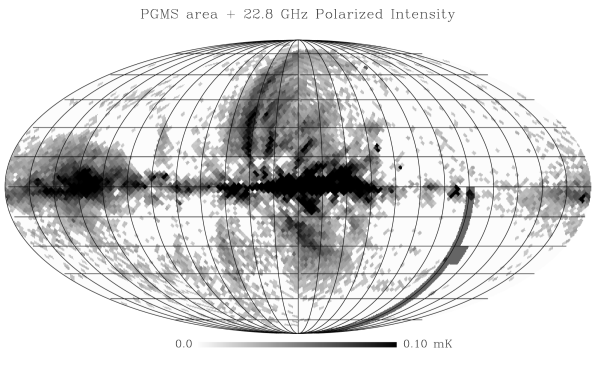
Figure 2: The PGMS strip (dark gray) plotted on the WMAP polarized intensity map ($L=\sqrt{Q^{2}+U^{2}}$) at 22.8 GHz (Page et al., 2007) binned in $2^{\circ}$ pixels (HEALPIX pixelation with Nside=32). Pixels with S/N $<$ 3 have been blanked (white). The PGMS goes through a region clear of large emission structures avoiding contamination by major large local anomalies, such as the big radio loops and the fan region (centred at $l\sim 135^{\circ}$, $b\sim 0^{\circ}$). The big radio loops are structures large several tens of degrees, like loop-I which extends from the north Galactic pole down to the Galactic plane, with a possible continuation into the southern hemisphere. The map is in Galactic coordinates with longitude $l=0^{\circ}$ at centre and increasing leftward.

The selected meridian goes through one of the low emission regions of the sky identified using the WMAP data (Fig. 2, see also Carretti et al. 2006b) and is free of large local emission structures. The meridian also goes through the area of deep polarization observations of the BOOMERanG experiment (Masi et al., 2006); the 10° extension near $b=-35^{\circ}$ is positioned to best cover that field.

At long wavelengths, measurements of Galactic polarized emission in regions of high rotation measure are corrupted by Faraday depolarization. At 1.4 GHz Faraday depolarization is significant up to Galactic latitudes $|b|<40$–$50\degr$ (Carretti et al., 2005a) where $RM>20$ rad/m². At 2.3 GHz this $RM$ limit increases to $60$ rad/m², allowing a clear view of polarized emission over all high Galactic latitudes and well into the upper part of the disc.

The observations were made in four sessions from January 2006 to September 2007 with the Parkes S-band Galileo receiver, named after NASA’s Jupiter exploration probe for which the Parkes telescope and this receiver were used for down-link support (Thomas et al., 1997). The receiver responds to left- and right-handed circular polarization, whose cross-correlation gives Stokes parameters $Q$ and $U$ (e.g. Kraus 1986). This scheme provides more protection against total-power (gain) fluctuations than the alternative: a receiver responding directly to the linearly polarized signals.

The original feed used for the Galileo mission has been replaced by a wide-band corrugated horn, highly tapered to reduce sidelobes and the response to ground emission. The feed illuminates the dish with a 20 dB edge taper and the first side-lobe is 30 dB below the main beam.

The ATNF’s Digital Filter Bank 1 (DFB1) was used to produce all four Stokes parameters, $I$, $Q$, $U$, and $V$. DFB1 was equipped with an 8-bit ADC and configured to give 256 MHz spectrum with 128 2-MHz channels. Spectra are generated using polyphase filters that provided high spectral channel isolation. The isolation between adjacent channels is 72 dB, an enormous improvement over the 13 dB isolation of Fourier-based correlators. This, in combination with the high sample precision, gives excellent protection against RFI leaking from its intrinsic frequency to other parts of the measured spectrum. This is valuable in the 13-cm band as strong RFI can be present. Recording spectra with spectral resolution greater than required for the polarimetry analysis has allowed efficient removal of RFI-effected channels, maximising the effective useful bandwidth. Data were reduced to 30 8-MHz channels. The RFI removal typically yielded an effective total bandwidth of 160 MHz.

The source B1934-638 was used for flux calibration assuming the polynomial model by Reynolds (1994) for an accuracy of 5%. The polarization response was calibrated using the sources 3C 138 and PKS 0637-752, whose polarization states were determined using the Australia Telescope Compact Array (ATCA) with an absolute error of $1^{\circ}$. The statistical error of our polarization angle calibration is $0.5^{\circ}$. The astronomical IAU convention for polarization angles is used: angles are measured from the local northern meridian, increasing towards the east. It is worth noting that this differs from the convention used in the WMAP data, for which the polarization angle increases westwards. The unpolarized source B1934-638 was also used to measure the polarization leakage, for which we measure a value of 0.4%. The off-axis instrumental polarization due to the optics response is about 1%.

The use of a system with both $Q$ and $U$ as correlated outputs mitigates gain fluctuation effects. To check the level of a 1/f noise component in the data we observed the South Celestial Pole (SCP), thereby avoiding azimuth (AZ) and elevation (EL) dependent variations of atmospheric and ground emissions. Remaining variations in the signal arise from intrinsic atmospheric changes and receiver fluctuations. Power spectra of the $Q$ and $U$ time-series are almost flat with no evidence of a 1/f component down to 3 mHz (see Fig. 3). This confirms that the system is stable and characterised by white noise up to 7-min time scales, sufficient for the duration of our scans.

Figure 3: Power spectra of $Q$ (top) and $U$ (bottom) time series for a south Celestical pole observation. Both spectra are mostly flat with no evidence of a 1/f component up to 3 mHz.

The Galactic meridian was observed in 16 $5^{\circ}\times 5^{\circ}$ fields and one $10^{\circ}\times 10^{\circ}$ field. The fields are named PGMS-XX, where XX is the Galactic latitude of the field centre. Each field except PGMS-02 includes a $1^{\circ}$ extension along $b$ at the north edge for an actual size of $5^{\circ}\times 6^{\circ}$ and an overlap of $5^{\circ}\times 1^{\circ}$ with the next northern field.

The fields were observed with sets of orthogonal scans to give $l$– and $b$–maps (scans along Galactic longitude and latitude, respectively). Each field was observed with 101 latitude scans ($b$–maps) and 121 longitude scans ($l$–maps) spaced by 3 arcmin to ensure full Nyquist sampling of the beam (FWHM = 8.9 arcmin). The same sample spacing was used along each scan by scanning the telescope at $3^{\circ}$/min with a 1-second integration time.

One full set of $l$– and $b$–maps were observed for the 6 disc fields at latitude $|b|<30^{\circ}$ and the $10^{\circ}\times 10^{\circ}$ field, giving final a sensitivity of $\sim 0.5$ mK per beam-sized pixel. Over the ten high latitude fields ($|b|>40^{\circ}$), where a weaker signal was expected, two full passes were made to give a sensitivity of $\sim 0.3$ mK per beam-sized pixel.

Prior to map-making, a linear baseline fit was removed from each scan and the ground emission contribution was estimated and cleaned up by the procedure described in Section 3.

The map-making procedure is based on the algorithm by Emerson & Gräve (1988), which combines $l$– and $b$–maps in Fourier space and recovers the power along the direction orthogonal to the scan, otherwise lost through the baseline removal. The algorithm is highly efficient and effectively removes residual stripes.

Table 1 summarises the main features of the PGMS observations.

Table 1: Main features of the PGMS observations.

Central frequency	2300 MHz
Effective bandwidth	240 MHz
Useful bandwidth1	160 MHz
FWHM	$8.9$ arcmin
Channel bandwidth	8 MHz
Central Meridian	$l_{0}=254^{\circ}$
Latitude coverage	$b=[-90^{\circ},0^{\circ}]$
Area size	$5^{\circ}\times 90^{\circ}$
Pixel size	$3\arcmin\times 3\arcmin$
Observation runs	Jan 2006
	Sep 2006
	Jan 2007
	Sep 2007
$Q$, $U$ beam-size pixel rms sensitivity (halo fields)	0.3 mK
$Q$, $U$ beam-size pixel rms sensitivity (disc fields)	0.5 mK
1 After RFI channel flagging.

3 Ground emission

Ground emission can seriously affect continuum observations, especially in our halo fields where the emission has a brightness of only a few mK. Our tests have shown that the highest ground emission occur in the Zenith cap at elevations above $60^{\circ}$ where large fluctuations are observed in the data. Even though not yet fully understood, the most likely reason is the loss of ground shielding by the upper rim of the dish at large elevations. The receiver is located at the prime focus and is shielded by the dish up to this elevation, receiving only atmospheric contributions from beyond the upper rim. Above this limit the ground becomes visible, contributing a ground component that rapidly varies as the telescope scans. To avoid this contamination all PGMS observations were limited to the elevation range EL = $[30^{\circ},60^{\circ}]$, between the lower limit of the telescope’s motion and this region of ground sensitivity.

Even though these precautions have significantly reduced the effect, some contamination is still present in the halo fields, requiring us to develop a procedure to estimate and clean the ground contribution.

3.1 Estimate and cleaning procedure

The procedure is based on making a map of the ground emission in the AZ–EL reference frame. Any AZ–EL bin gathers the contributions of data taken at different Galactic coordinates and the weak sky emission is efficiently averaged out. Since the PGMS meridian goes through low emission regions, its high latitude data are ideal for such an aim. The smooth behaviour of the ground emission enables the use of large bins, which further helps average out the sky component. We therefore use a bin size of $\Delta$EL = 1deg in EL and average over 8 degrees in Azimuth. The binning is performed in the instrument reference frame before the correction for parallactic angle.

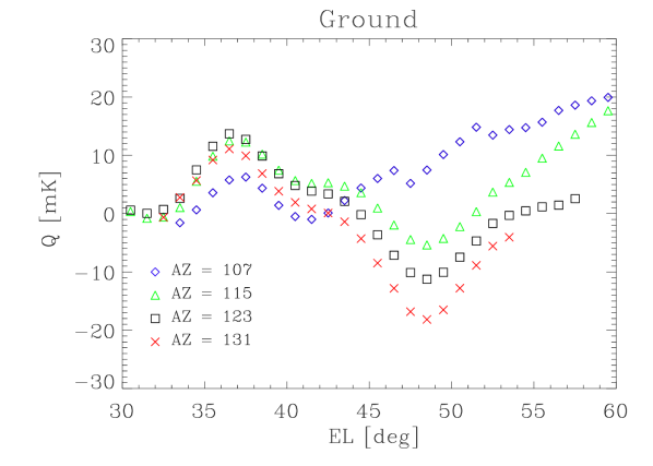
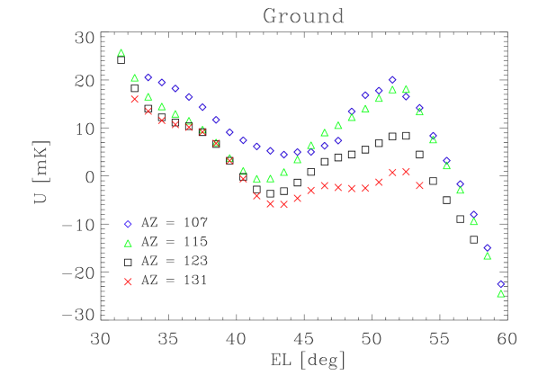
Figure 4: Examples of azimuth cuts of the ground emission maps of both $Q$ (top) and $U$ (bottom) from the 2300 MHz channel of the September 2007 observations.

For a given 8 degree AZ bin we smooth the map along the EL direction. This reduces the residual local deviations that are mainly due to strong point sources. We use a quadratic running fit: for each EL bin, we fit the 7 bins centred at it with a 2-degree polynomial, and the bin value is then replaced with the fit result at the bin position.

In the Azimuthal direction the data are sufficiently smooth that no fit is necessary in that dimension. We therefore shift our 8 degree azimuth averages by 1 degree increments, performing the elevation fit for each 1 degree bin. This results in a map of the ground emission in the AZ-EL frame with a bin size of 1 degree in both Azimuth and Elevation.

The ground emission contamination mainly comes from the far lobes, which are frequency dependent. We generate ground emission maps for each frequency channel. A set of these maps is generated at each observing session. They are checked for constancy of ground emission before a grand average set is formed from all observations.

Fig. 4 shows example AZ cuts in the 2300 MHz spectral channel. Over a range of about $30\degr$ in both AZ and EL the ground emission varies by less than 50 mK, smaller by an order of magnitude than ground emission variations reported for other polarization surveys (e.g. Wolleben et al. 2006). We attribute this low response to ground emission to the high edge tapering of the S-band feed and its consequent small sidelobes.

Finally, the sky emission measurements, observed on a 3-arcminute grid, were cleaned of ground emission using the model just described. For each sky measurement, the ground emission at its actual (AZ, EL) was obtained by linear interpolation through a standard Cloud-In-Cell technique (Hockney & Eastwood, 1981).

3.2 Cleaning procedure tests

The low emission fields in the halo have been observed twice giving two independent maps taken in different runs and at different AZ and EL. That way, they are contaminated by different ground emission enabling us to test the cleaning procedure and estimate the residual contamination. The error map can be estimated as half the difference of the two maps, in which the sky is cancelled, leaving the noise and any residual (unmodelled) ground emission.

An example is given in Fig. 5 in which one of the fields with lowest emission is shown: PGMS-87. The images show Stokes $Q$ (left) and $U$ (right) of both the observed (top) and difference maps (bottom).

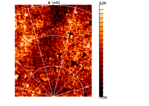
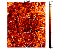
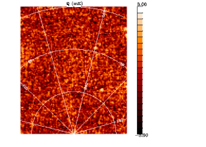
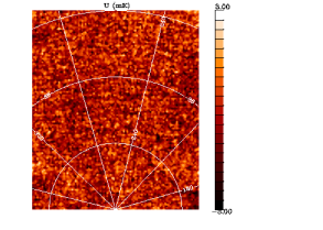
Figure 5: $Q$ (left) and $U$ images (right) of the observed (top) and difference maps (bottom) of the field PGMS-87 ($b$=[-84^∘, -90^∘]). No smoothing is applied for a resolution of FWHM=8.9’. Position coordinates are Galactic latitude and longitude; the brightness unit is mK, the intensity colour scales are linear.

The difference maps are clearly dominated by white noise, indicating that most of the ground emission has been removed at the level needed to measure the sky signal, and that the residual ground emission does not contribute significantly to the error budget. That residual can be seen as faint shadows of large scale structure in the difference maps.

These visual impressions of the ground emission removal we know quantify by measuring the angular power spectra of both the sky and the difference map. Fig. 6 reports the mean of the $E$– and $B$–mode power spectra – ($E$+$B$)/2 – which is the most complete description of the polarized emission.

The spectrum of the sky signal is dominated by the diffuse emission at low multipole $\ell$, where it follows a power law $C_{\ell}\propto\ell^{\beta}$ with a steep slope ($\beta<-2.0$). A flattening occurs at the high–$\ell$ end due to both noise and a point source contribution. A white noise spectrum would be flat ($C_{\ell}$ = constant).

The difference spectrum also follows a power law, but is much flatter than the sky signal. The best fit slope is $\beta_{\rm noise}=-0.70\pm 0.06$, which, although not pure white noise, is close to the ideal $\beta_{\rm noise}=0$. Furthermore, the difference between sky signal and noise increases at large angular scale, giving a rapidly increasing S/N.

The ground emission has a smooth behaviour that makes the largest scales the most susceptible to contamination. On a scale of 2^∘ the rms fluctuation of the difference map is $N_{2^{\circ}}=60$ $\mu$K, a factor 2.5 larger than that expected from white noise (24 $\mu$K), but much smaller than the sky signal (few mK).

This field (PGMS-87) is the worst with regard to ground emission residuals; over all fields, angular spectral slopes $\beta_{\rm noise}$ fall in the range [-0.7, 0.0] and the rms noise on the 2-degree scale $N_{2^{\circ}}$ lie in [24, 60] $\mu$K. The mean values over all fields are $\bar{\beta}_{\rm noise}=-0.4$ and $\bar{N}_{2^{\circ}}=43$ $\mu$K. Once the pure white noise component is subtracted, the effective contribution by only ground emission can be estimated in $\bar{N}_{{\rm grnd},2^{\circ}}=36$ $\mu$K. With such results the impact of the ground emission may be considered marginal on the final mapping.

4 PGMS maps

Figure 6: Power spectrum of the mean ($E$+$B$)/2 of $E$– and $B$–Modes measured for the PGMS-87 polarized emission: sky emission (diamonds), difference map (stars) and best fit curves (dashed).

Maps of the Stokes parameters $Q$, $U$ and the polarized intensity $L$ of the PGMS meridian are shown in Fig. 7, 8, and 9, while Fig. 10 displays the whole $10\degr\times 10\degr$ field (PGMS-34). All images are smoothed with a Gaussian filter of FWHM $=6\arcmin$ to give a better idea of the sensitivity on beam-size scale, for an effective resolution of FWHM $=10.7\arcmin$. All data at latitude $|b|>30^{\circ}$ are plotted with the same intensity range to show clearly the power and morphological differences. The disc fields ($|b|<30^{\circ}$) require a more extended scale. The two strongest sources present in our data (Pic A and NGC 612 in field PGMS-34 and PGMS-77, respectively) have been blanked before the map generation of their fields. Without blanking, the high brightness range causes the map-making procedure to generate artefacts.

The disc has the strongest emission, extending to latitude $|b|\sim 20\degr$ with little variation of emission power. At higher latitudes, the emission starts to decrease up to the halo where it settles on levels one order of magnitude lower.

The clear visibility of the bright polarized disc emission and its contrast with the fainter halo is a new result, not apparent from previous observations carried out at lower frequencies where the disc is strongly depolarized up to $|b|\sim 30\degr$. This allows us to locate the disc-halo boundary in polarization, which has not been visible so far because of either strong depolarization (at 1.4 GHz) or insufficient sensitivity (at 23 GHz). A more quantitative analysis is given in Section 5, but the visual inspection of the maps clearly shows that it starts at $|b|\sim 20\degr$.

The emission of the halo has a smooth behaviour with the power mostly residing on large angular scales. The disc emission is also smooth, at least at latitudes higher than $|b|=6\degr$–$7\degr$. Closer to the Galactic plane the pattern has a more patchy appearance, suggestive of Faraday depolarization effects being significant at 2.3 GHz.

This supports the view that Faraday depolarization effects are marginally significant in the disc, and are relevant only in a narrow belt a few degrees wide across the Galactic plane.

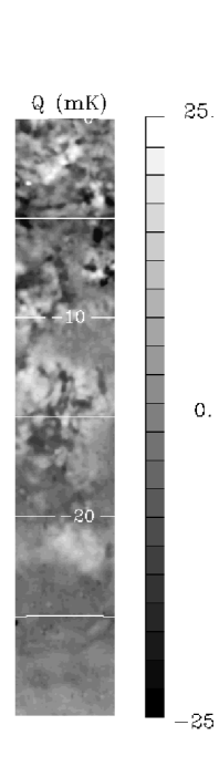
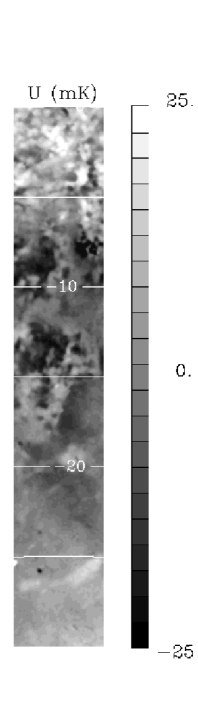
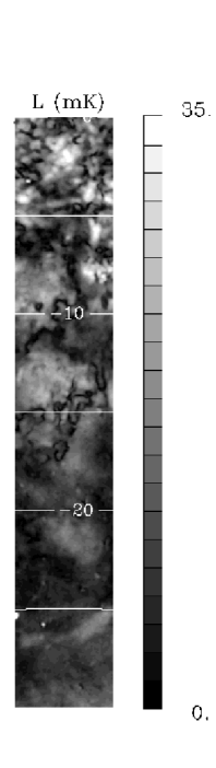
Figure 7: $Q$ (left), $U$ (mid), and polarized intensity $L=\sqrt{Q^{2}+U^{2}}$ images (right) of the six PGMS fields in the latitude range $b=[-30\degr,0\degr]$ (PGMS-27 through PGMS-02). Position coordinates are Galactic latitude; the brightness unit is mK.

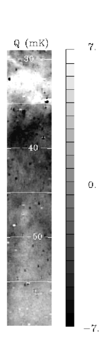
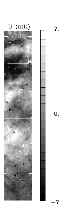
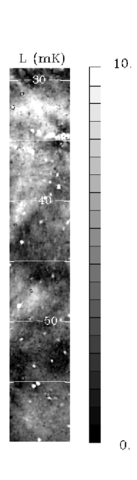
Figure 8: As for Fig. 7 but in the range $b=[-60\degr,-30\degr]$ (PGMS-57 through PGMS-34: of the latter only the $5\degr$ across the meridian $l=254\degr$ are imaged). Position coordinates are Galactic latitude; the brightness unit is mK.

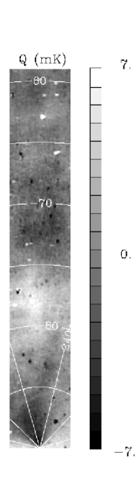
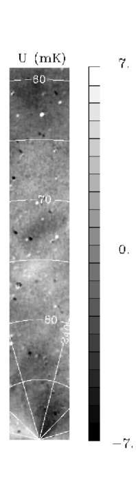
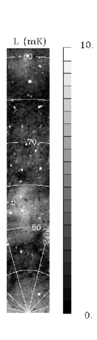
Figure 9: As for Fig. 7 but in the range $b=[-90\degr,-60\degr]$ (PGMS-87 through PGMS-62). Position coordinates are Galactic latitude and longitude; the brightness unit is mK.

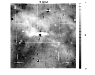
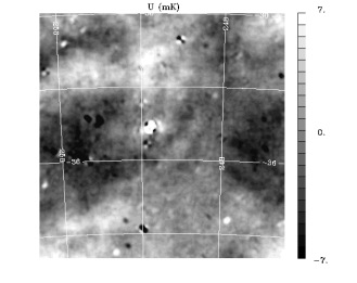
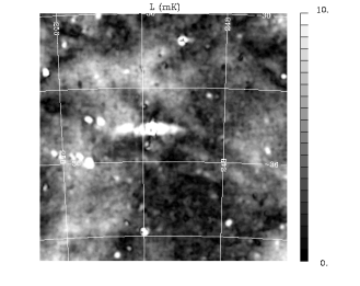
Figure 10: $Q$ (top), $U$ (mid), and $L$ images (bottom) of the whole $10\degr\times 10\degr$ fields (PGMS-34). Position coordinates are Galactic latitude and longitude; the brightness unit is mK.

Table 2: Polarization flux limits $S_{p}^{\rm lim}$ used to selected the polarized sources. The chosen limits are latitude dependent.

$b$-range	$S_{p}^{\rm lim}$ [mJy]
$[-10\degr,0\degr]$	40
$[-20\degr,-10\degr]$	30
$[-30\degr,-20\degr]$	20
$[-40\degr,-30\degr]$	15
$[-90\degr,-40\degr]$	10

Several polarized point sources are visible, especially in the halo where the diffuse emission fluctuations are smaller. To enable a cleaner analysis of the diffuse component the sources are identified, fitted and subtracted from the maps. Each source is located by a 2D-Gaussian fit of the stronger component, either $Q$ or $U$. Its position is then fixed in the fit of the second and weaker component to improve the fit robustness. A polarization flux limited selection is applied with threshold set to ensure $S/N$ ratios of at least 5. The amplitude of fluctuations in the maps is dominated by sky emission (rather than by the instrument sensitivity), which varies along the PGMS meridian. The threshold we use is therefore a function of Galactic latitude, running from 10 mJy at high latitudes up to 40 mJy near the Galactic plane (Table 2).

In this work, the point source identification is carried out only for cleaning purposes. The catalogue and a detailed analysis of their properties are subject of a forthcoming paper (Bernardi et al. 2010, in preparation).

5 Angular power spectra

The angular power spectra (APS) of $E$– and $B$–Mode of the polarized emission have been computed for each field. They account for the 2-spin tensor nature of the polarization and give a full description of the polarized signal and its behaviour across the range of angular scales. In addition, the $E$– and $B$–Modes are the quantities predicted by the cosmological models enabling a direct comparison with the CMB.

To cope with both the non-square geometry and the blanked pixels at the locations of the two brightest sources, we use a method based on the two-point correlation functions of the Stokes parameters $Q$ and $U$ described by Sbarra et al. (2003). The correlation functions are estimated on the $Q$ and $U$ maps of the regions as

$$\tilde{C}^{X}(\theta)=X_{i}X_{j}\hskip 28.45274ptX=Q,U$$ (1)

where $X_{i}$ is the emission in pixel $i$ of map $X$, and $i$ and $j$ identify pixel pairs at distance $\theta$. Data are binned with pixel-size resolution. Power spectra $C^{E,B}_{\ell}$ are obtained by integration

$$C^{E}_{\ell}=W_{\ell}^{P}\int^{\pi}_{0}[\tilde{C}^{Q}(\theta)F_{1,\ell 2}(\theta)+\tilde{C}^{U}(\theta)F_{2,\ell 2}(\theta)]\sin(\theta)d\theta$$ (2)

$$C^{B}_{\ell}=W_{\ell}^{P}\int^{\pi}_{0}[\tilde{C}^{U}(\theta)F_{1,\ell 2}(\theta)+\tilde{C}^{Q}(\theta)F_{2,\ell 2}(\theta)]\sin(\theta)d\theta$$ (3)

where $F_{1,\ell m}$ and $F_{2,\ell m}$ are functions of Legendre polynomials (see Zaldarriaga 1998 for their definition), and $W_{\ell}^{P}$ is the pixel window function accounting for pixel smearing effects.

Since the emission power is best described by the quantity $\ell(\ell+1)C_{\ell}/(2\pi)$, hereafter we will denote an angular spectrum following a power law behaviour $C_{\ell}\propto\ell^{\beta}$ as

• flat, if $\beta=-2.0$: power equally distributed across the angular scales;

• steep, if $\beta<-2.0$: large scales dominate the power budget;

• inverted, if $\beta>-2.0$: small scales dominates.

We tested the procedure using simulated maps generated from a known input power spectrum by the procedure synfast of the software package HEALPix (Górski et al., 2005). The input spectra are power laws with different slopes; for each slope we generated 100 simulated maps and compute their APS. The mean of the 100 APS reproduced the input spectrum and its slope correctly, with the exception of an excess at the largest scales, mainly at the first two multipole bands. $E$– and $B$–Mode are related to the polarization angle pattern and this excess is likely due to the discontinuity of the pattern abruptly interrupted at the area borders. To account for this we corrected our spectra for the fractional excess estimated from the simulation as the ratio between the mean of the computed and input spectra.

For a cleaner measure of the diffuse component, the point sources are subtracted from the polarization maps.

The $E$– and $B$–mode spectra $C^{E}_{\ell}$ and $C^{B}_{\ell}$ have been computed for the 17 fields along with their mean $C_{\ell}^{(E+B)/2}=(C_{\ell}^{E}+C_{\ell}^{B})/2$. Artificial fluctuations are generated on $E$ and $B$ spectra because of the limited sky coverage of the individual areas, but their mean suffers less from that effect and is a more accurate estimator if the power is distributed equally between the two modes, as is the case for Galactic emission. In addition, $C^{(E+B)/2}_{\ell}$ gives a full description of the polarized emission which the two individual spectra cannot give separately. Therefore we mostly use the mean spectrum ($E$+$B$)/2 to investigate emission behaviour and properties in the following analysis.

Fig. 11 shows $C^{(E+B)/2}_{\ell}$ for all the fields. As an example of all three spectra, Fig. 12 shows those of the two fields PGMS-52, which is from the low emission halo, and PGMS-34, our biggest field and the area observed by the BOOMERanG experiment. All spectra are shown without correction for the window functions.

Figure 11: Angular power spectra $C_{\ell}^{(E+B)/2}$ of the 17 PGMS fields. Both the measured spectra (diamonds) and the best fit curve (solid) are plotted.

Figure 12: Angular power spectrum of $E$–Mode (top), $B$–Mode (mid), and their mean ($E$+$B$)/2 of the two fields PGMS-52 (left) and PGMS-34 (right). Both the measured spectra (diamonds) and the best fit curve (solid) are plotted.

Table 3: Best fit amplitude $C^{X}_{200}$ (referenced to $\ell=200$) and angular spectral slope $\beta^{X}$ of the PGMS fields ($X=E,B,(E+B)/2$ denoting $E$–, $B$–Mode, and ($E$+$B$)/2, respectively).

Field	$C^{E}_{200}$ [$\mu$K2]	$\beta^{E}$	$C^{B}_{200}$ [$\mu$K2]	$\beta^{B}$	$C^{(E+B)/2}_{200}$ [$\mu$K2]	$\beta^{(E+B)/2}$
PGMS-02	$4500\pm 280$	$-1.69\pm 0.04$	$4860\pm 880$	$-1.90\pm 0.13$	$4610\pm 540$	$-1.76\pm 0.09$
PGMS-07	$3850\pm 380$	$-1.77\pm 0.07$	$4120\pm 340$	$-1.75\pm 0.06$	$4030\pm 340$	$-1.76\pm 0.06$
PGMS-12	$2800\pm 200$	$-1.86\pm 0.05$	$3160\pm 410$	$-1.82\pm 0.09$	$3070\pm 240$	$-1.85\pm 0.06$
PGMS-17	$2090\pm 260$	$-2.00\pm 0.10$	$1270\pm 140$	$-1.67\pm 0.08$	$1840\pm 190$	$-1.91\pm 0.08$
PGMS-22	$550\pm 100$	$-2.54\pm 0.17$	$246\pm 39$	$-2.60\pm 0.16$	$376\pm 31$	$-2.39\pm 0.08$
PGMS-27	$287\pm 58$	$-2.41\pm 0.24$	$131\pm 19$	$-2.17\pm 0.19$	$263\pm 20$	$-2.51\pm 0.09$
PGMS-34	$183.5\pm 8.5$	$-2.54\pm 0.07$	$171.8\pm 9.0$	$-2.46\pm 0.07$	$180.0\pm 7.1$	$-2.51\pm 0.06$
PGMS-42	$79\pm 11$	$-2.76\pm 0.19$	$61.9\pm 6.3$	$-2.24\pm 0.14$	$74.1\pm 4.0$	$-2.57\pm 0.08$
PGMS-47	$59.8\pm 7.7$	$-2.91\pm 0.20$	$49.7\pm 4.3$	$-2.56\pm 0.13$	$56.3\pm 3.1$	$-2.78\pm 0.08$
PGMS-52	$47.9\pm 4.4$	$-2.74\pm 0.13$	$42.7\pm 5.9$	$-2.36\pm 0.17$	$51.3\pm 3.2$	$-2.66\pm 0.08$
PGMS-57	$46.7\pm 3.4$	$-2.62\pm 0.10$	$16.6\pm 2.2$	$-2.54\pm 0.21$	$32.4\pm 1.7$	$-2.61\pm 0.07$
PGMS-62	$28.9\pm 3.1$	$-3.27\pm 0.22$	$19.1\pm 3.4$	$-3.35\pm 0.40$	$24.1\pm 1.9$	$-3.27\pm 0.17$
PGMS-67	$15.6\pm 2.0$	$-2.17\pm 0.19$	$5.4\pm 1.1$	$-2.23\pm 0.34$	$12.6\pm 1.6$	$-2.35\pm 0.20$
PGMS-72	$40.1\pm 4.1$	$-3.08\pm 0.16$	$14.9\pm 2.8$	$-2.81\pm 0.33$	$29.7\pm 2.7$	$-3.03\pm 0.15$
PGMS-77	$41.6\pm 6.4$	$-3.05\pm 0.27$	$33.8\pm 3.6$	$-2.47\pm 0.16$	$38.4\pm 4.5$	$-2.75\pm 0.19$
PGMS-82	$16.2\pm 3.3$	$-2.36\pm 0.35$	$18.0\pm 3.0$	$-2.51\pm 0.27$	$21.7\pm 2.8$	$-2.57\pm 0.21$
PGMS-87	$26.9\pm 1.6$	$-2.21\pm 0.07$	$11.3\pm 0.7$	$-1.74\pm 0.07$	$19.9\pm 1.4$	$-2.08\pm 0.09$

In most fields the spectra follow a power law behaviour that flattens at the high multipole end because of the noise contribution. Exceptions are the four fields closest to the Galactic plane (PGMS-17 to PGMS-02) where a power law modulated by the beam window function dominates everywhere. .

We fit the angular power spectra to a power law modulated by the beam window function $W_{\ell}^{B}$ for the synchrotron component and a constant term $N$ for the noise:

$$C_{\ell}^{X}=\left[C_{200}^{X}\left(\frac{\ell}{200}\right)^{\beta^{X}}W_{\ell}^{B}+N\right]\,W_{\ell}^{P}\,,$$ (4)

where $C_{200}^{X}$ is the spectrum at $\ell=200$ and $X=E,B,(E+B)/2$ denoting $E$–Mode, $B$–Mode, and their mean ($E$+$B$)/2. Possible residual contributions by point sources are accounted for by the constant term.

Plots of the best fits are shown in Fig. 11 and 12, while the parameters of the synchrotron component are reported in Table 3.

To analyse the behaviour of the synchrotron component, the power law component of the best fit spectra are plotted together in Fig. 15 where they are also extrapolated to 70 GHz for comparison with the CMB signal. To determine the spectral index for the frequency extrapolation we computed a map of spectral index of the polarized synchrotron emission (Fig. 13) using the all-sky polarization surveys at 1.4 GHz (Wolleben et al., 2006; Testori et al., 2008) and 22.8 GHz (WMAP, Hinshaw et al. 2009). The index distribution at high Galactic latitudes ($|b|>30^{\circ}$) peaks at $\alpha_{\rm pol}=-3.21$ with dispersion $\Delta\alpha_{\rm pol}=0.15$ (Fig. 14). This is consistent with the analysis of the WMAP-5yr data by Gold et al. (2009), who find a polarized synchrotron spectral index of $\alpha_{\rm WMAP}=-3.1$ in the WMAP frequency range, and that of Bernardi et al. (2004) of total intensity data ($\alpha_{I}=-3.1$ in the range 1.4–22.8 GHz). We therefore assume a spectral index of $\alpha_{\rm synch}=-3.1$ for extrapolations up to the CMB frequency window. This assumption is somewhat conservative and gives some margin to our conclusions.

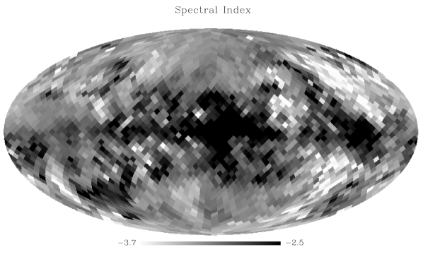
Figure 13: Map of frequency spectral index of the polarized synchrotron emission computed using the all-sky polarization maps at 1.4 GHz (Wolleben et al., 2006; Testori et al., 2008) and at 22.8 GHz (WMAP-5yr, Hinshaw et al. 2009)

Figure 14: Distribution of the spectral indexes reported in Fig. 13.

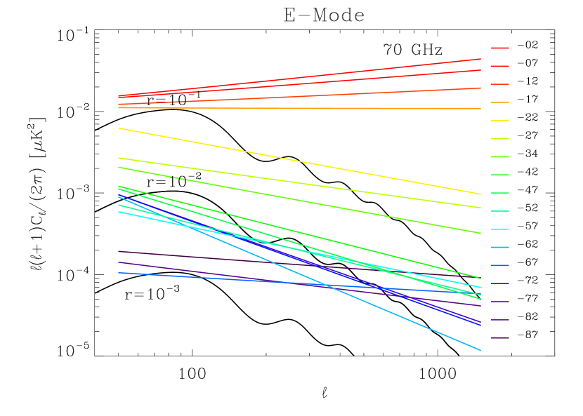
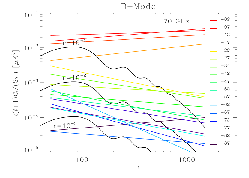
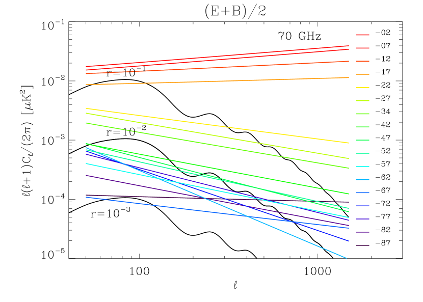
Figure 15: Best fits to the spectra of $E$–Mode (top), $B$–Mode (mid), and their mean ($E$+$B$)/2 (bottom) of all PGMS fields. The plot reports only the power law component which describes the synchrotron emission. All PGMS fields are plotted together for a direct comparison of the behaviour with the Galactic latitude. The colour code goes from blue throughout red by a rainbow palette for the areas from the south Galactic pole (PGMS-87) throughout the Galactic plane (PGMS-02), respectively. The spectra are scaled to 70 GHz for a comparison with the CMB signal (frequency spectral index $\alpha=-3.1$). CMB $B$–Mode spectra for different values of tensor-to-scalar power ratio $r$ are shown for comparison. The quantity plotted here is $\ell(\ell+1)/(2\pi)*C^{X}_{\ell}$, which provides a direct estimate of the power distribution through the angular scales: a flat spectrum means the power is evenly distributed; a decreasing spectrum (steep) is dominated by the largest scales; a rising spectrum (inverted) is dominated by the smallest scales.

Figure 16: Angular spectral slopes of the PGMS fields plotted against the field’s centre latitude for $E$–Mode (top), $B$–Mode (mid), and ($E$+$B$)/2.

Distinguishing fields in terms of their spectral slopes, Fig. 15 and Fig. 16 show the presence of two well defined regions:

• The high and mid latitude fields ($b$ = [-90$\degr$, -20$\degr$]), with steep spectra ($\beta<-2.0$); slopes are distributed over the wide range $\beta\sim$ [-3.0, -2.0] (except for a few outliers). There is no clear trend with latitude and the slopes are rather uniformly distributed. The median is $\beta_{\rm med}^{(E+B)/2}=-2.6$ (Table 4). The dispersion $\sigma_{\beta^{(E+B)/2}}=0.24$ is significantly larger than the individual measurement errors, meaning that this wide spread is an intrinsic property of the synchrotron emission at these latitudes.

• The low latitude fields ($b=[-20\degr,~{}0\degr]$), which show inverted spectra ($\beta>-2.0$); the slopes lie in a much narrower range ($\beta^{(E+B)/2}=[-1.90,-1.75]$) with dispersion $\sigma_{\beta^{(E+B)/2}}=0.08$ (Table LABEL:slope_l:Tab). All spectra have mean and median slope $\bar{\beta}^{X}=\beta^{X}_{\rm med}=-1.8$, which can be considered the typical value of this region.

This change from steep to inverted spectra is quite sudden and clearly separates two different environments: the mid-high latitudes, characterised by a smooth emission with most of the power on large angular scales, and the disc fields, whose power is more evenly distributed with a slight predominance of the small scales.

Table 4: Mean ($\bar{\beta}^{X}$), median ($\beta^{X}_{\rm med}$), and dispersion ($\sigma_{\beta}$) of the angular slopes at mid-high Galactic latitudes for all the three spectra $X=E,B,(E+B)/2$.

MID-HIGH latitudes
X	$\bar{\beta}^{X}$	$\beta^{X}_{\rm med}$	$\sigma_{\beta^{X}}$
$E$	-2.67	-2.62	0.34
$B$	-2.39	-2.46	0.27
$(E+B)/2$	-2.57	-2.57	0.24

Table 5: As for Table 4 but for low Galactic latitudes.

LOW latitudes
X	$\bar{\beta}^{X}$	$\beta^{X}_{\rm med}$	$\sigma_{\beta^{X}}$
$E$	-1.83	-1.81	0.14
$B$	-1.78	-1.78	0.10
$(E+B)/2$	-1.82	-1.80	0.08

Does this change indicate an intrinsic feature of the polarized emission of the disc, or is it the effect of Faraday modulation, which transfers power from large to small angular scales in the low latitude fields? The answer is unclear with the information available, but some points can be noted. In the disc the ISM is more turbulent than in the halo and the intrinsic emission might have more power on small angular scales. In addition, the low-latitude lines of sight go through much more ISM including more distant structures; these are expected to give more power to the small angular scales. Also the smooth emission of the two highest latitude disc fields (PGMS-12 and PGMS-17) make the presence of significant Faraday depolarization unlikely. Finally, we have computed the power spectrum of the individual frequency channels to search for a possible variation of the angular slope with frequency. Since the lowest frequencies would be more affected, steeper spectra at highest frequencies would support the presence of FR effects. We find that all the four disc fields have non-significant slope variation compatible with zero within 1.0–1.5 sigma, with the only exception of PGMS-02 which approaches 2-sigma. All these points support the view that the structure of the low-latitude polarized emission derives from the intrinsic nature of the synchrotron emitting regions close to the plane, and is not imposed by Faraday depolarization along the propagation path.

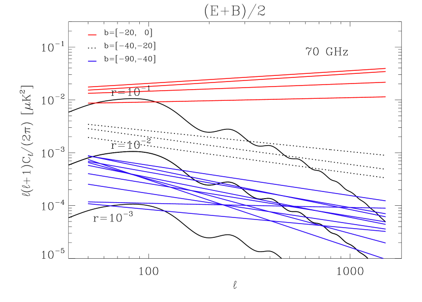
Figure 17: As bottom panel of Fig. 15, but with spectra grouped according to latitude region. The disc fields (solid, red: $b=[-20\degr,0\degr]$) are clearly distinguished by their spectral slopes and higher amplitudes, and the fields in the transition region (dotted, black: $b=[-40\degr,-20\degr]$) have amplitudes quite distinct from both the disc and halo fields (solid, blue: $b=[-90\degr,-40\degr]$).

Considering the amplitude distribution of the PGMS fields, we further divide the mid-high latitude region identified above into an halo ($b=[-90\degr,-40\degr]$) and transition region ($b=[-40\degr,-20\degr]$). Thus we identify three distinct latitude sections: two main regions (disc and high latitudes) well distinguished by both emission power and structure of the emission, and an extended transition about $20\degr$ wide connecting them. Fig. 17 reports the spectra for all field, showing how they belong to the three regions, which:

• Halo ($b=[-90\degr,-40\degr]$): the emission is weak here and, scaled to 70 GHz, is between the peaks of CMB models with $r=10^{-3}$ and $r=10^{-2}$. The weakest fields (PGMS-87 and PGMS-67) match models with $r=10^{-3}$. The fluctuations from field-to-field dominate with no clear trend with latitude. A weak trend might be present with the emission power increasing toward lower latitudes, but the effect is a minor in comparison to the dominant field-to-field fluctuations.

• Galactic disc ($b=[-20\degr,0\degr]$): the emission is stronger, about two orders of magnitude brighter than that of the halo. Within the area there is no large variation of the emission power, but slight increase toward the Galactic plane is evident.

• Transition strip ($b=[-40\degr,-20\degr]$): here a transition between the faint high latitudes and the bright disc occurs. This is clearer at large scales, where the northernmost field (PGMS-22) is almost as bright as the weakest disc field (PGMS-17) and the southermost field approaches the upper end of the halo brightness range.

An important consequence is the identification of a clear transition between disc and halo. The sudden change in the angular spectral slope at $|b|\sim 20\degr$ and the approximately constant emission power from the Galactic plane up to that transition clearly separate the $20\degr$ equatorial zone from the higher latitudes. Characterised by a more complex structure of the ISM this area can be associated with the Galactic disc.

A second environment characterised by steep spectra and low emission is clearly present for $|b|>40\degr$. Both angular slope and amplitude exhibit wide fluctuations without any clear trend with latitude. We consider this high Galactic latitude section as a single environment with regard to its polarized synchrotron emission properties. Characterised by a smoother emission and simpler ISM structure, this area we associate with the Galactic halo.

Table 6: Best fit amplitude $C^{X}_{\ell}$ and angular spectral slope $\beta^{X}$ of the mean spectrum of the PGMS halo section ($X=E,B,(E+B)/2$ denotes $E$–, $B$–Mode, and ($E$+$B$)/2, respectively).

Field	$C^{E}_{200}$ [$\mu$K2]	$\beta^{E}$	$C^{B}_{200}$ [$\mu$K2]	$\beta^{B}$	$C^{(E+B)/2}_{200}$ [$\mu$K2]	$\beta^{(E+B)/2}$
PGMS HALO	$40.7\pm 3.2$	$-2.65\pm 0.10$	$28.5\pm 3.0$	$-2.64\pm 0.12$	$35.5\pm 2.9$	$-2.60\pm 0.09$

Figure 18: Mean of the power spectra of the halo fields ($b=[-40\degr,-90\degr]$) for $E$–Mode (top), $B$–Mode (mid), and their mean ($E$+$B$)/2 (bottom). Both the mean of the measured spectra (diamonds) and its best fit curve (solid) are plotted.

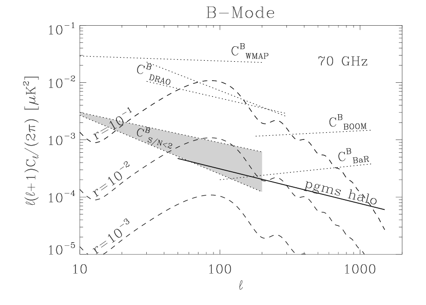
Figure 19: Best fit of the mean halo spectrum $C^{(E+B)/2}_{\ell}$ scaled to 70 GHz (solid) alongside CMB $B$–Mode spectra for different $r$ values (dashed). The mean synchrotron contamination at all high Galactic latitudes in also shown for comparison ($C^{B}_{\rm WMAP}$) together with the previous estimates in other low emission regions: $C^{B}_{S/N<2}$ (shaded area), $C_{\rm DRAO}$, $C^{B}_{\rm BOOM}$, and $C^{B}_{\rm BaR}$ (see Fig. 15 for details).

The emission of the halo section is very weak. In spite of large fluctuations, once scaled to 70 GHz the synchrotron component is equivalent to $r$ values between $1\times 10^{-3}$ and $7\times 10^{-3}$, which matches the weakest areas observed so far in polarization. It is worth noticing that PGMS fields PGMS-87 and PGMS-67 have the weakest polarized synchrotron emission observed so far.

The high Galactic latitudes above 40$\degr$ are thus just one environment, at least in a low emission region not contaminated by local anomalies like the area intersected by PGMS. This is very important for CMB investigations, since it tells that, in principle, it is possible to find large areas with optimal conditions (extended over $50\degr$, in the PGMS case).

It is thus important to measure the mean emission properties of the entire halo section ($|b|>40\degr$). The mean spectrum of the 10 halo fields and its best fit are plotted in Fig. 18; Table 6 gives the best fit parameters; the extrapolation to 70 GHz is shown in Fig. 19.

The angular slope is $\beta^{X}\sim-2.6$ for all the three spectra $E$, $B$, and ($E$+$B$)/2 and is thus be considered the typical slope of the halo section. Note that this matches the slope measured at high latitudes by WMAP at 22.8 GHz (Page et al., 2007), indicating that the power distribution through the angular scales is the same at 2.3 and 22.8 GHz. This further argues against the significance of Faraday depolarization, which would have transferred power from large to small scales and made the angular spectra frequency dependent.

Once scaled to 70 GHz, the amplitude is equivalent to

$$r_{\rm halo}=(3.3\pm 0.4)\times 10^{-3},$$ (5)

roughly in the middle of the range covered by the individual fields. As mentioned earlier, this is a very low level and corresponds to the faintest areas observed previously, which thus seem to be more the normal condition of the low emission regions rather than lucky exceptions.

Finally, the field PGMS-34 deserves mention as the area observed by the experiment BOOMERanG. It lies in the transition region, and although at the high-latitude end of this zone, has emission about five times greater than fields in the halo. It is suitable for measuring the stronger $E$-mode (the aim of the 2003 BOOMERanG flight), but our results identify more suitable fields for detecting the B-mode.

6 Dust emission in the PGMS halo section

The dust emission is the other most significant foreground for CMB observations. It has a positive frequency spectral index and dominates the foreground budget at high frequency.

An estimate of the local dust contribution in the same portion of halo covered by the PGMS is thus important to understand the overall limits of a CMB $B$–Mode detection in that area.

However, no polarized dust emission has been detected over the PGMS region, and even the total intensity dust map of WMAP is noise dominated in that area. We therefore use the Finkbeiner, Davis & Schlegel (1999) model of the total intensity dust emission applying an assumed polarization fraction. First, we generate maps at 94 GHz using their model-8 for each of the 10 PGMS fields at $|b|>40\degr$. The temperature power spectra of each are then computed and averaged together to estimate the mean conditions of the whole $5\degr\times 50\degr$ section. Fig. 20 shows both the mean spectrum and its best fit, whose parameters are reported in Table 7. Within the errors, the angular slope matches well that of the synchrotron.

Figure 20: Temperature power spectrum of the dust emission model at 94 GHz in the halo section of the PGMS ($b=[-90\degr,-40\deg]$). The spectrum is the mean of those computed in the individual PGMS fields. Both the mean of the computed spectra (diamonds) and its best fit curve (solid) are plotted. The latter is a power law with slope $\beta^{T}_{d}=-2.50\pm 0.14$ (see text and Table 7).

Table 7: Best fit amplitude $C^{T}_{200}$ and angular spectral slope $\beta^{T}_{d}$ of the mean Temperature dust spectrum at 94 GHz in the halo section of the PGMS ($|b|>40\degr$).

Field	$C^{T}_{200}$ [$\mu$K2]	$\beta^{T}_{d}$
PGMS halo Dust	$(12.0\pm 1.4)\times 10^{-6}$	$-2.50\pm 0.14$

The total polarized spectrum is estimated from this temperature spectrum assuming a polarization fraction $f_{\rm pol}=0.10$, as inferred for high Galactic latitudes from the Archeops experiment data (Beno$\hat{\rm\i}$t et al., 2004; Ponthieu et al., 2005). The spectrum is further divided by two to account for an even distribution of power between $E$– and $B$–Mode, a reasonable assumption for the Galactic emission.

For frequency extrapolations, we use a single Planck function modulated by a power law $T_{d}\propto\nu^{\alpha_{d}}/(e^{h\nu\over kT}-1)$ with index $\alpha_{d}=2.67$ and temperature $T=16.2$ K, which reproduces the Finkbeiner et al. (1999) model well in the range $[70,150]$ GHz. It is worth noticing that at 94 GHz that function is well approximated by a power law with index $\alpha_{d}^{\rm PL}=1.5$, consistent with the 5-yr WMAP result of $\alpha_{d}^{\rm WMAP}=1.8\pm 0.3\pm 0.2$ (statistical and systematic error, Gold et al. 2009).

Figure 21: Estimates of the dust polarized emission in the halo section of the PGMS at 70 GHz (solid). The best fit to the temperature spectrum is used assuming a dust polarization fraction $f_{\rm pol}=0.10$ and then scaled to 70 GHz. The synchrotron emission spectrum estimated in Section 5 is shown for comparison (dotted), as well as the CMB $B$–Mode spectra for three different $r$ values.

Our estimate of the $B$–Mode polarized dust spectrum at 70 GHz is given in Fig. 21. At this frequency the two components of Galactic polarized emission are approximately equal, and so the total polarized foregound is at a minimum. This frequency is mildly dependent on assumed polarized fraction of the dust component: alternate assumptions of five percent or twenty percent shift the frequency of minimum to 80 GHz and 60 GHz respectively.

This result is similar to that of the general high Galactic latitudes and suggests that the synchrotron-to-dust power ratio is only marginally dependent on the strength of the Galactic emission.

7 Limits on $\mn@boldsymbol{r}$

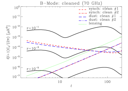
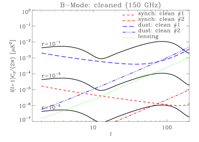
Figure 22: Residual contaminations after foreground cleaning in the PGMS halo section at 70 (left) and 150 GHz (right) for synchrotron (red) and dust emission (blue). Results for both the two cleaning methods described in text are shown. The gravitational lensing contribution is also shown assuming that cleaning has reduced its contribution by a factor 10 in the power spectrum (green).

Table 8: Detection limits of $r$ at 3-sigma C.L. ($\delta r$) at 70 and 150 GHz in the PGMS halo area and in a 2500-deg² region assumed to have equivalent foreground contamination (see text). Results for both cleaning types described in the text are reported.

Area	clean type	$\delta r$ (70 GHz)	$\delta r$ (150 GHz)
PGMS	clean #1	$2.2\times 10^{-3}$	$8.0\times 10^{-3}$
PGMS	clean #2	$1.5\times 10^{-3}$	$5.5\times 10^{-3}$
2500-deg2	clean #1	$1.2\times 10^{-3}$	$4.2\times 10^{-3}$
2500-deg2	clean #2	$0.5\times 10^{-3}$	$1.8\times 10^{-3}$

To estimate the detection limits of $r$ in the presence of the foreground contamination in the PGMS halo section, we consider an experiment with resolution $\theta_{\rm cmb}=1^{\circ}$ at the CMB frequency channel to have adequate sensitivity at the $\ell\sim 90$ peak.

We also account for the cleaning provided by foreground separation techniques. We consider the two cases discussed by Tucci et al. (2005):

1. cleaning by subtracting the foreground map scaled to higher frequencies using just one frequency spectral index for all pixels. It is a coarse method and represents a worst case. The residual contamination depends on the spread of spectral indices in the area. We use $\Delta\alpha_{s}=0.15$ for the synchrotron component (Section 5; see also Bernardi et al. 2004; Gold et al. 2009), and assume the same dispersion for the dust emission ($\Delta\alpha_{d}=0.15$). We refer to this method as clean #1.

2. cleaning by foreground subtraction, but assuming knowledge of the frequency spectral index for any individual pixel. In this case the amplitude of the residual contamination depends on the measurement error of the frequency slopes. Here we assume a combination of the PGMS data with a synchrotron channel at 22 GHz onboard the CMB experiment with resolution $\theta_{\rm s}=1^{\circ}$ and sufficient sensitivity to give $S/N=5$. For the dust emission, we assume that the CMB experiment includes a dust channel at 350 GHz with a sensitivity to allow a $S/N=5$ and resolution scaled from the CMB channel ($\theta_{\rm d}=\theta_{\rm cmb}\nu_{\rm cmb}/\nu_{\rm d}$, where $\nu_{\rm cmb}$ and $\nu_{\rm d}$ are the frequencies of the CMB and dust channel). We refer to this method as clean #2.

These two methods are at the two ends of cleaning capabilities (#1 is coarser and less efficient, #2 is finer and more efficient), so give a good idea of the range of possible performance.

The left panel of Fig. 22 shows the residual contaminations left by these two methods at 70 GHz in the PGMS halo section using the method of Tucci et al. (2005). The effect of method #1 is to reduce the amplitude of the contamination but preserve the shape of the power spectrum (for instance, the synchrotron residual preserves the angular spectral index of -2.6). Method #2 gives comparable results at the $\ell\sim 90$ CMB peak, but has a flat white–noise–like spectrum which performs much better on large angular scales. While the simpler clean #1 looks appropriate as the target is the peak at $\ell\sim 90$, the clean #2 is better suited for the reionization bump at larger scales.

With such low levels of residual foreground contribution the effects of gravitational lensing become a dominant part of the contamination budget. Its subtraction is therefore also required to realise the benefit of the low Galactic emission of the PGMS strip. Gravitational lensing effects can be cleaned using high resolution data (10 arcmin or better, Seljak & Hirata 2004) and here we assume that it can be reduced by 10 fold (Seljak & Hirata 2004).

The Fisher information matrix is used to estimate the detection limits (Tegmark, Taylor & Heavens, 1997; Tegmark, 1997). If $r$ is the only parameter to be measured, (other cosmological parameters being provided by Temperature and $E$–Mode spectrum from other experiments such as WMAP or PLANCK), the Fisher matrix reduces to the scalar

$$\mathcal{F}_{rr}=\sum_{\ell}\frac{1}{(\Delta C_{\ell}^{B})^{2}}\left(\frac{\partial C_{\ell}^{B}}{\partial r}\right)^{2}$$ (6)

and the rms error on $r$ is

$$\sigma_{r}=\mathcal{F}_{rr}^{-1/2}.$$ (7)

The uncertainty $\Delta C_{\ell}^{B}$ of the $B$–mode spectrum is a function of the CMB spectrum $C_{\ell}^{B,{\rm cmb}}$ and the cleaning residuals of synchrotron, dust, and gravitational lensing:

$$\Delta C_{\ell}^{B} = \sqrt{\frac{2}{(2\ell+1)\Delta\ell\,f_{\rm sky}}}\,C_{\ell}^{B,{\rm cmb}}$$ (8)

$$+ \left(C_{\ell}^{B,{\rm synch-res}}+C_{\ell}^{B,{\rm dust-res}}+C_{\ell}^{B,{\rm lens-res}}\right),$$

where $\Delta\ell$ is the width of the multipole bins and $f_{\rm sky}$ is the sky coverage fraction. As a set of cosmological parameters we use the best fits of the 5-yr WMAP data release (Komatsu et al., 2009).

At 70 GHz the detection limits of $r$ in the PGMS halo region is $\delta r\sim 2\times 10^{-3}$ (3-sigma C.L.) for both cleaning methods (Table 8). This is a very low level which makes the PGMS strip an excellent target for CMB experiments and enables accessing levels of $r$ much lower than previously estimated for areas of comparable size (e.g. Tucci et al. 2005; Verde et al. 2006, who used higher foreground levels estimated from total intensity data). An important point is that there is only a marginal benefit from using the more sophisticated cleaning method. For a 250-deg² area most of the sensitivity resides in the $\ell\sim 90$ peak, where the dominant residual is the gravitational lensing and a better cleaning of the other contaminants is not critical.

This result is therefore quite robust since it is based on actual measurements of the foreground contamination in a specific area and is marginally dependent on the cleaning method. Moreover, the leading residual term is the gravitational lensing, giving a good margin against errors in our dust polarization fraction assumption.

It is also important to estimate $\delta r$ for 150 GHz, a frequency that, although far from the foreground minimum, is preferred by experiments based on bolometric detectors. However, as shown in Fig. 22, right panel, the major residual at this frequency is dust emission, making the result dependent on the assumed dust polarization fraction $f_{\rm pol}$. A value of $f_{\rm pol}=0.10$ gives the limit $\delta r=6$–$8\times 10^{-3}$ (Table 8), while the goal of the most advanced sub-orbital experiments planned for the next years ($r\sim 1\times 10^{-2}$) is still achievable under the reasonable assumption that $f_{\rm pol}<0.12$.

The PGMS halo region is a narrow strip 50^∘ long and it is unlikely that its optimal conditions are confined to its 5^∘ width. Therefore we consider that a larger area, say of $50\degr\times 50\degr$ extent, could be identified with properties comparable to those of the PGMS halo region. Such an area, about 6 per cent of the sky, matches in size the southern portion of the low emission region identified in the WMAP data (Carretti et al., 2006b).

The detection limit achievable over such an area drops to $\delta r=5\times 10^{-4}$ (3-sigma C.L.) if method #2 is applied, or $\delta r=1.2\times 10^{-3}$ under the coarser method #1 (Table 8).

Note that in this case there is a significant difference between the two cleaning methods, justifying the use of the more sophisticated method #2. This is because the larger area makes measurement of the lowest multipole components relevant, where method #1 is not effective.

8 Summary and Conclusions

The PGMS has mapped the radio polarized emission at all Galactic latitudes in a 5 degree strip at a frequency sufficiently high not to be affected by Faraday depolarization and with sufficient sensitivity to detect the signal in low emission regions. It is the largest area observed so far at high Galactic latitude uncontaminated by large local structures.

This has enabled us to investigate the behaviour of the polarized emission with latitude by computing the polarized angular power spectrum in 17 fields from the Galactic plane to the South Galactic pole. We can distinguish three latitude sections: two main regions well distinguished by both brightness and structure of the emission (disc and halo), and an extended transition connecting them. In detail they are:

1.  The halo at high Galactic latitudes ($b=[-90\degr,-40\degr]$) characterised by low emission fields with steep spectra (angular slope $\beta=[-3.0,-2.0]$), that is smooth emission dominated by large scale structures. The slope is almost uniformly distributed within a wide range, with median $\beta_{\rm med}=-2.6$.

2.  A transition region at mid-latitudes ($b=[-40\degr,-20\degr]$) whose angular spectra are steep like those of the halo, but shows an increase of the emission power with decreasing latitude.

3.  The disc at low latitudes ($b=[-20\degr,0\degr]$) characterized by inverted spectra with slopes in a narrow range of median $\beta_{\rm med}=-1.8$. The amplitudes are two orders of magnitude brighter than in the halo and the power gradually increases towards the Galactic plane.

The change in the angular slope around $b=-20\degr$ is abrupt and identifies a sharp disc-halo transition from the smooth emission of the mid-high latitudes to the more complex behaviour of the disc; this is likely related to the more turbulent and complex structure of the ISM in the disc.

The halo section has no clear trend with latitude of either emission power or angular slope, and, at least along the meridian sampled by PGMS, can be considered a single environment. This is very important for CMB investigations, as it indicates that it is possible to find large areas with optimal conditions for seeking the $B$–Mode.

The synchrotron emission of the whole halo section is very weak. Once scaled to 70 GHz it is equivalent to $r=3.3\times 10^{-3}$, so that an experiment aiming for a detection limit of $\delta r=0.01$–0.02 would need no synchrotorn foreground cleaning.

The dust component is also faint and equal to the synchrotron emission at 60–80 GHz for polarization fractions between 5 and 20 %. The frequency of minimum foreground in this low emission region is thus similar to that found with WMAP for the general high Galactic latitudes (75% of the sky). If confirmed in other regions, this would imply both that the dust-synchrotron power ratio is rather independent of the brightness of the Galactic emission and the frequency of minimum foreground nearly independent of the sky position.

We estimate the $r$ detection limit of this area accounting for the use of foreground cleaning procedures. We apply both a coarse and a more refined method. The Galactic emission is so low that the dominant residual contamination is from gravitational lensing, even assuming a 10-fold reduction of the lensing foreground from cleaning. For both the two cleaning methods the detection limit is $\delta r\sim 2\times 10^{-3}$ (3-sigma C.L.) if the CMB $B$–Mode search is conducted at 70 GHz. This result provides a sound basis for investigating the $B$–Mode. The detection limit we have found here is even better than the goals of the most advanced sub-orbital experiments ($r\sim 0.01$, e.g.: SPIDER, EBEX, and QUIET, Crill et al. 2008; Grainger et al. 2008; Samtleben 2008) and proves that there exists at least one area of the sky where it is realistic to carry out investigations of the $B$–mode down to very low limits of $r$.

At 150 GHz the detection limit rises, but is still better than $\delta r=0.01$ assuming a reasonable dust polarization fraction ($f_{\rm pol}<$ 12%).

These results are valid in the area actually observed by our survey. However, the PGMS halo section is extended over $50\degr$ along one dimension and it is unlikely that its excellent conditions are confined to its $5\degr$ width. We have explored the likely results from a larger $50\degr\times 50\degr$ area, having properties similar to those of the PGMS halo section. In such a region the $r$ detection limit would drop to $\delta r=5\times 10^{-4}$ (3-sigma) at 70 GHz.

It is worth noticing that the gravitational lensing needs to be cleaned to take advantage of the low Galactic emission of the PGMS halo section. This can be effectively carried out only with high resolution data ($10^{\prime}$ or finer, Seljak & Hirata 2004) and the design of CMB experiments should comply with that rather than be limited to 1-degree to fit the peak at $\ell\sim 90$.

The results obtained here might suggest a review of plans to detecting the CMB $B$–Mode and associated investigations of the inflationary scenarios. While the detection limit is limited to $\delta r=1\times 10^{-2}$ by the detector array size and sensitivity, observations at 150 GHz might be sufficient if conducted in an area like the PGMS with clear advantages of using the currently best detectors (bolometers) and of an experiment more compact than at 70 GHz. Moreover, the synchrotron emission is sufficiently weak at 150 GHz not to require any cleaning, which removes the need for low frequency channels to measure it. Experiments like EBEX and BICEP already match such conditions, not only because of the design choices, but also because their target areas intersects the PGMS strip (Grainger et al., 2008; Chiang et al., 2009).

A deeper detection limit, down to $\delta r=2\times 10^{-3},$ could be reached by a sub-orbital experiment observing the same area but with the CMB channel shifted to 70 GHz. The inclusion of a channel at a lower frequency would be required to measure the synchrotron component. Finally, detections limits down to $\delta r=5\times 10^{-4}$ coiuld be achieved by observing at 70 GHz in a large area of $50\degr\times 50\degr$ having the PGMS foreground levels. The location of the most suitable region must be determined, a task that can be accomplished by the forthcoming large foreground surveys like the S-band Polarization All Sky Survey (S-PASS), or the C-band All Sky Survey (C-BASS).

These limits are comparable to the goals of the space missions currently under study such as B-POL and CMBPol (de Bernardis et al., 2008; Baumann et al., 2008), but with the significant advantage that such an area is still sufficiently compact to be observable by a sub-orbital experiment. The limit $r\sim 1\times 10^{-3}$ is an important threshold for the inflationary physics since it is about the lower limit of the important class of inflationary models with low degree of fine tuning (Boyle et al., 2006). Our study shows that this threshold may be reached with an easier and cheaper sub-orbital experiment rather than a more complex space mission, making this goal more realistically achievable with a smaller budget and in a shorter time than that required to develop space-borne equipment.

The PGMS data will be made available at the site http://www.atnf.csiro.au/people/Ettore.Carretti/PGMS

References

- Amarie et al. (2005) Amarie M., Hirata C., Seljak U., 2005, PRD, 72, 123006
- Baumann et al. (2008) Baumann D., et al., 2008, arXiv:0811.3911 [astro-ph]
- Beck (2008) Beck R., 2008, in ”The UV Window to the Universe”, eds. A.I. Gomez de Castro and M. Castellanos, Ap&SS, in press, arXiv:0711.4700 [astro-ph]
- Benot et al. (2004) Benot A., et al., 2004, A&A, 424, 571
- Bernardi et al. (2004) Bernardi G., Carretti E., Fabbri R., Sbarra C., Poppi S., Cortiglioni S., Jonas J.L., 2004, MNRAS, 351, 436
- Bernardi et al. (2006) Bernardi G., Carretti E., Sault R.J., Cortiglioni S., Poppi S., 2006, MNRAS, 370, 2064
- Boyle et al. (2006) Boyle L.A., Steinhardt P.J., & Turok N., 2006, Phys. Rev. Lett. 96, 111301
- Brown et al. (2007) Brown J.C., Haverkorn M., Gaensler B.M., Taylor A.R., Bizunok N.S., McClure-Griffiths N.M., Dickey J.M., Green A.J., 2007, ApJ, 663, 258
- Brown et al. (2009) Brown M.L., et al, 2009, ApJ, 705, 978
- Beuermann et al. (1985) Beuermann K., Kanbach G., & Berkhuijsen E.M., 1985, A&A, 153, 17
- Carretti et al. (2005a) Carretti E., Bernardi G., Sault R.J., Cortiglioni S., & Poppi S., 2005a, MNRAS, 358, 1
- Carretti et al. (2005b) Carretti E., McConnell D., McClure-Griffiths N.M., Bernardi G., Cortiglioni S., & Poppi S., 2005b, MNRAS, 360, L10
- Carretti et al. (2006a) Carretti E., Poppi S., Reich W., Reich P., Fürst E., Bernardi G., Cortiglioni S., Sbarra C., 2006a, MNRAS, 367, 132
- Carretti et al. (2006b) Carretti E., Bernardi G., Cortiglioni S., 2006b, MNRAS, 373, L93
- Chiang et al. (2009) Chiang H.C., et al, 2009, submitted to ApJ, arXiv:0906.1181 [astro-ph.CO]
- Crill et al. (2008) Crill B.P., et al., 2008, in Space Telescopes and Instrumentation 2008: Optical, Infrared, and Millimeter, Eds. J.M. Oschmann Jr., M.W.M. de Graauw & H.A. MacEwens, Proc. of SPIE, 7010, 70102P
- de Bernardis et al. (2008) de Bernardis P., Bucher M., Burigana C., Piccirillo L., 2008, Exp. Astron., in press, arXiv:0808.1881 [astro-ph]
- Emerson & Gräve (1988) Emerson D.T., Gräve R., 1988, A&A,190, 353
- Finkbeiner et al. (1999) Finkbeiner D.P., Davis M., Schlegel D.J., 1999, ApJ, 524, 867
- Frick et al. (2001) Frick P., Stepanov R., Shukurov A., & Sokoloff D., 2001, MNRAS, 325, 649
- Gaensler et al. (2001) Gaensler B.M., Dickey J.M., McClure-Griffiths N.M., Green A.J., Wieringa M.H., & Haynes R.F., 2001, ApJ, 549, 959
- Gold et al. (2009) Gold B., et al., 2009, ApJS, in press, arXiv:0803.0715 [astro-ph]
- Górski et al. (2005) Górski K.M., et al., 2005, ApJ, 622, 759
- Grainger et al. (2008) Grainger W., et al., 2008, in Millimeter and Submillimeter Detectors and Instrumentation for Astronomy IV, Eds. W.D. Duncan, W.S. Holland, S. Withington, J. Zmuidzinas, Proc. of SPIE Vol. 7020 70202N-2
- Han (2002) Han J.L., 2002, in Astrophysical Polarized Backgrounds, eds. S. Cecchini, S. Cortiglioni, R. J. Sault, C. Sbarra, AIP Conf. Ser., 609, 96
- Han (1997) Han J.L., Manchester R.N., Berkhuijsen E.M., & Beck R., 1997, A&A, 322, 98
- Han et al. (2006) Han J.L., Manchester R.N., Lyne A.G., Qiao G.J., van Straten W., 2006, ApJ, 642, 868
- Haverkorn et al. (2006) Haverkorn, M., Gaensler B.M., McClure-Griffiths N.M., Dickey, J.M., Green A.J., 2006, ApJS, 167, 230
- Hinshaw et al. (2009) Hinshaw G., et al., 2009, ApJS, 180, 225
- Hockney & Eastwood (1981) Hockney R.W., Eastwood J.W., 1981, Computer Simulation Using Particles (New York: McGraw-Hill)
- Jansson et al. (2009) Jansson R., Farrar G.R., Waelkens A.H., & Ensslin T.A. 2009, JCAP, 7, 21
- Kamionkowski & Kosowsky (1998) Kamionkowski M., Kosowsky A., 1998, PRD, 57, 685
- Komatsu et al. (2009) Komatsu E., et al., 2009, ApJS, 180, 330
- Kraus (1986) Kraus J.D., 1986. Radio Astronomy (Ed. Cygnus Quasar Books: Powell, OH)
- Lange (2008) Lange A., 2008, in CMB component separation and the physics of foregrounds, http://planck.ipac.caltech.edu/content/ForegroundsConference/presentationsForWEB/58_andrewLange.pdf
- La Porta et al. (2006) La Porta L., Burigana C., Reich W., Reich P., 2006, A&A, 455, L9
- Masi et al. (2006) Masi S., et al., 2006, A&A, 458, 687
- Page et al. (2007) Page L., et al, 2007, ApJS, 170, 335
- Peiris et al. (2003) Peiris H.V., et al, 2003, ApJS, 148, 213
- Ponthieu et al. (2005) Ponthieu N., et al., 2005, A&A, 444, 327
- Reynolds (1994) Reynolds J.E. 1994, ATNF Tech. Doc. Ser. 39.3040
- Samtleben (2008) Samtleben D., in Cosmology 2008, Proc. of the 43rd Rencontres de Moriond, in press, arXiv:0806.4334 [astro-ph]
- Sbarra et al. (2003) Sbarra C., Carretti E., Cortiglioni S., Zannoni M., Fabbri R., Macculi C., Tucci M., 2003, A&A, 401, 1215
- Seljak & Hirata (2004) Seljak U., Hirata C.M., 2004, PRD, 69, 043005
- Sun et al. (2008) Sun X.H., Reich W., Waelkens A., Enßlin T.A., 2008, A&A, 477, 573
- Tegmark (1997) Tegmark M., 1997, PRD, 56, 4514
- Tegmark et al. (1997) Tegmark M., Taylor A.N., Heavens A.F., 1997, ApJ, 480, 22
- Testori et al. (2008) Testori J.C., Reich P., Reich W., 2008, A&A, 484, 733
- Thomas et al. (1997) Thomas B.M., Schafer J.T., Sinclair M.W., Kesteven M.J., Hall P.J., 1997, IEEE Antennas & Propagation Magazine, 39, 54
- Tucci et al. (2005) Tucci M., Martínez-González E., Vielva P., Delabrouille J., 2005, MNRAS, 360, 935
- Verde et al. (2006) Verde L., Peiris H.V., Jimenez R., 2006, JCAP, 1, 19
- Wolleben et al. (2006) Wolleben M., Landecker T.L., Reich W., Wielebinski R., 2006, A&A, 448, 411
- Zaldarriaga (1998) Zaldarriaga M., 1998, Ph.D. Thesis, M.I.T., astro-ph/9806122