Tunable Locally-Optimal Geographical Forwarding in Wireless Sensor Networks with
Sleep-Wake Cycling Nodes

Abstract

We consider a wireless sensor network whose main function is to detect certain infrequent alarm events, and to forward alarm packets to a base station, using geographical forwarding. The nodes know their locations, and they sleep-wake cycle, waking up periodically but not synchronously. In this situation, when a node has a packet to forward to the sink, there is a trade-off between how long this node waits for a suitable neighbor to wake up and the progress the packet makes towards the sink once it is forwarded to this neighbor. Hence, in choosing a relay node, we consider the problem of minimizing average delay subject to a constraint on the average progress. By constraint relaxation, we formulate this next hop relay selection problem as a Markov decision process (MDP). The exact optimal solution (BF (Best Forward)) can be found, but is computationally intensive. Next, we consider a mathematically simplified model for which the optimal policy (SF (Simplified Forward)) turns out to be a simple one-step-look-ahead rule. Simulations show that SF is very close in performance to BF, even for reasonably small node density. We then study the end-to-end performance of SF in comparison with two extremal policies: Max Forward (MF) and First Forward (FF), and an end-to-end delay minimising policy proposed by Kim et al. [1]. We find that, with appropriate choice of one hop average progress constraint, SF can be tuned to provide a favorable trade-off between end-to-end packet delay and the number of hops in the forwarding path.

I Introduction

An important application of wireless sensor networks (WSN) is dense embedded sensing for the purpose of detecting certain infrequently occuring events, such as failures in a large structure, or intrusion into a secure region. Such an event can occur anywhere in a large WSN, and once an event is detected, the alarm needs to be rapidly sent to the sink for further action. In such WSNs, typically the nodes rely on batteries, or energy harvested from their surroundings, and, hence, need to be extremely parsimonius in their use of energy. In order to conserve energy, the nodes operate in sleep-wake cycles; when a node wakes up it performs sensing, and also can assist in forwarding any alarm packets towards the sink. In this paper, we consider the situation in which the sleep-wake cycles of nodes are not synchronized. In such a setting, stateful routing is not possible. Instead, if the nodes know their own locations and that of the sink, then it is possible to dynamically select forwarding nodes that are successively nearer to the sink. This is called geographical routing, and has been widely studied as a simple scalable approach for routing in sensor networks [2, 3, 4, 5]. For the purpose of location determination, low cost GPS devices are now becoming available, and can be incorporated in the nodes; alternatively, approximate localization algorithms based on various geometrical principles can also be used (see, for example, [6, 7]. For a survey on routing and localization, see [8, 9]. In this paper we assume that nodes know their exact locations and also the location of the sink.

The relay node selection problem: In geographical forwarding, in our setting, there arises the problem of optimal relay node selection, which we now discuss. One approach is that of greedy forwarding, in which an intermediate node forwards the packet to its neighbor node that makes maximum progress towards the sink. This scheme is referred to as Most Forward within Radius (MFR) ([2, 3]). If the node density is large such that every node has a neighbor that is closer to the sink than itself, then the greedy approach can find routes close to the minimum hop paths. Following a minimum hop path is beneficial since it reduces the number of times the network needs to transmit the packet.

However, when the nodes are sleep-wake cycling in an asynchronous manner there is a trade-off between the delay in relay node selection and the progress made towards the sink. For example, if MFR is implemented, then for an intermediate node to forward the packet to a relay node that makes the maximum progress towards the sink, the intermediate node will need to wait for all its neighbors closer to the sink than itself to wake up. This will result in an increase in the delay of the alarm that is being forwarded. In fact, a counterpart to the MFR policy could be the policy that forwards the packet to the first node that wakes up and is nearer to the sink than the intermediate node. In this paper we call this latter policy First Forward (FF), and the MFR policy, simply, Max Forward (MF).

In this paper we study the above trade-off for the following one hop relaying problem. A node needs to forward a packet to the sink. There is a set of neighbors of the node that are nearer to the sink than the node; the forwarding set. The nodes are asynchronously sleep-wake cycling according to a certain model. We seek policies for relay node selection so as to minimize the delay in determining the relay node, subject to a constraint on the progress made towards the sink. We assume that each node has at least one neighbor that is strictly closer to the sink than itself so that greedy forwarding will always find a path to sink. This is a reasonable assumption for large node densities.

Our contributions:

• The problem of minimizing average one hop delay subject to a constraint on the average progress made, when nodes wake up periodically, but not synchronously, is formulated as a Markov decision problem (MDP), and solved to yield the optimal policy which we call Best Forward (BF). See Section IV and Section V.

• In a mathematically simplified setting (i.i.d., exponentially distributed inter-wakeup times) the MDP approach is used to derive a threshold type policy, called Simplified Forward (SF). The threshold is a function of the constraint on progress, and the policy is to transmit to the first node which wakes up and makes a progress of more than the threshold. See Section VI. While such a policy has been proposed heuristically in previous works ([10, 11]), we have derived it from the MDP formulation and we show through simulations that the performance of this policy is close to that of BF. The simulation results are in Section VIII.

• Finally, we compare the end to end performance (average delay and hop counts) of the SF policy with the forwarding policy proposed by Kim et al. [1]. The approach of Kim et al. aims to achieve minimum average end-to-end delay, but at the expense of an initial configuration phase. The SF policy, however, does not need any global organization phase, and the progress constraint can be used to tune the end-to-end performance to suitably trade-off between end-to-end delay and the number of hops in the forwarding path. These results are reported in Section VIII.

II Related Work

Zorzi and Rao ([12]) consider a scenario similar to ours: geographical forwarding in a wireless mesh network in which the nodes know their locations, and are sleep-wake cycling. They propose GeRaF (Geographical Random Forwarding), a distributed relaying algorithm, whose objective is to carry a packet to its destination in as few hops as possible, by making as large progress as possible at each relaying stage. Thus, the objective is similar to the MFR algorithm, mentioned above ([2, 3]). For their algorithm, the authors obtain the average number of hops (for given source-sink distance) as a function of the node density. These authors do not consider the trade-off between relay selection delay and the progress towards the sink, which is a major contribution of our work.

Liu et al. ([11]) propose a relay selection approach as a part of CMAC, a protocol for geographical packet forwarding. With respect to the fixed sink, a node $i$ has a forwarding set consisting of all nodes that make progress greater than $r_{0}$ (an algorithm parameter). If $Y$ represent the delay until the first wake-up instant of a node in the forwarding set, and $X$ is the corresponding progress made, then, under CMAC, node $i$ chooses an $r_{0}$ that minimizes the expected normalized latency $\mathbb{E}[\frac{Y}{X}]$. The Random Asynchronous Wakeup (RAW) protocol ([10]) also considers transmitting to the first node to wake up that makes a progress greater than a threshold $Th$. Interestingly, this is also the structure of the optimal policy provided by one of our Markov decision process formulations.

Kim et al. ([1]) consider a dense WSN in which the traffic model and sleep-wake cycling are similar to ours. An occasional alarm packet needs to be sent, from wherever in the network it is generated, to the sink. The nodes are asynchronously sleep-wake cycling. The authors develop an optimal anycast scheme to minimize average end-to-end delay from any node $i$ to the sink. The optimization is also done over sleep-wake cycling patterns and rates. A dynamic programming approach is taken, with the stages being the number of hops to the sink. While the framework is similar to ours, Kim et al. do not consider the objective of spatial progress at each hop, which results in the reduction of hop counts along the forwarding paths, and thus in the reduction of node energy utilization. In our work, we have studied the trade-off, at a typical forwarding stage, between forwarding delay and the distance that the packet covers in the hop.

Rossi et al. ([13]) consider the problem of geographical forwarding in a wireless sensor network in which each node knows its hop distance from the sink. For each link, there is a link cost (for example, energy cost) for forwarding a packet over that link. Thus, there are two end-to-end cost criteria for a forwarding path: the total link cost of the path, and the number of hops in the path. When a node, say $i$, has a packet to forward to the sink, it has to consider the trade-off between cost reduction and hop distance reduction; note that cost can be reduced by forwarding the packet to a neighbor node with the same hop distance to the sink, but using which the total link cost could be lower. The information available at $i$ is the cost to all its neighbors, and the statistics of the costs-to-go from the neighbors. The major difference in our work is that we have a sequential decision problem at each stage, since the costs (wake-up delay) and rewards (progress towards the sink) are revealed as the nodes wake up, and only the statistics are known a priori.

Chaporkar and Proutiere ([14]) consider the problem of a transmitter that needs to transmit over one of several available channels. The transmitter can probe the channels to determine channel state information in order to encode its transmissions. The trade-off is between the time taken to probe and the throughput advantage of finding a good channel. Some important differences between their model and ours are the following. In our work the trade-off is between the time taken to wait for a relay to wake up, and the spatial progress the relay makes towards the sink. In [14], the transmitter can use an unprobed channel, whereas in our problem a relay that has not yet woken up cannot be used. In [14], the transmitter can probe the channels in an order that it can choose (e.g., the stochastically best channel first); in our problem the relays wake up in a random order that is not under the control of the transmitter. In [14] it is shown that if the use of an unprobed channel is not allowed then a one-step-look-ahead rule is optimal. This is similar to the solution we obtain for a simplified version of our model. Note that whereas the concern in [14] is only with one-step relaying, we also study how the one-step policy performs in terms of end-to-end objectives, namely, path delay and path hop count.

III System Model

III-A Node Deployment

$N$ identical sensor nodes are uniformly deployed in the square region $[0,L]^{2}$. We take $N$ to be a Poisson random variable of rate $\lambda L^{2}$ where $\lambda$ is the node density. Let $x_{i}$, $i=1,2,...,N$, be the locations of the nodes. Additional source and sink nodes are placed at fixed locations $x_{0}=(0,0)$ and $x_{N+1}=(L,L)$ respectively. Thus including the source and sink nodes, there are a total of $N+2$ nodes in the disk. $r_{c}$ is the communication range of each node. Two nodes $i$ and $j$ are called neighbors if and only if $|x_{i}-x_{j}|\leq r_{c}$. The distance between node $i$ and sink ($N+1$) is $L_{i}=|x_{N+1}-x_{i}|$.

III-B The Sleep-Wake Process

To conserve energy, each node performs periodic sleep-wake cycling. The sleep-wake times of the nodes are not synchronized. Since we are interested in studying the delay incurred in routing due to sleep-wake cycling alone, we neglect the transmission delay, propagation delay and other overhead delays. This means that if node $i$ has a packet to transmit to its neighboring node $j$, then $i$ can transmit immediately at the instant $j$ wakes up. We model this by taking the time for which a node stays awake to be zero.

More formally, let $T_{i}$, $i=1,2,...,N+1$ be i.i.d. random variables which are uniform on $[0,T]$, where $T$ is the period of the sleep wake cycle. Then node $i$ wakes up at the periodic instants $kT+T_{i},k\geq 0$. We define the waiting time for i to wake up at time $t$ as,

$$W_{i}(t)=\inf\{kT+T_{i}\geq t:k\geq 0\}-t$$ (1)

III-C Forwarding Rules and Assumptions

Forwarding rules dictate the actions a node can take when it has to transmit. We are interested in decentralized policies where a node can take decisions only by observing the activities in its neighborhood (i.e., the disk of radius $r_{c}$ centered around the node of interest). In this regard we impose some restrictions on the network.

Traffic Model: There is a single packet in the network which is to be routed from the source to sink. At time $0$, the packet is given to the source and the routing process begins. The nodes which get the packet for forwarding are called relay nodes. The packet traverses a sequence of relay nodes to eventually reach the sink, at which time the routing ends. Thus there is a single flow and further the flow consists of only one packet. This set up is reasonable, because in sensor networks we can assume that the events are sufficiently separated in time and/or location so that the flows due to two events do not intersect. To avoid multiple packet transmission by different nodes detecting the same event, the nodes can resolve among themselves to select one node (say the one closest to the sink), which can then transmit. Further, the information about an event comprises its location, and possibly target classification data, which along with some control bits can be easily incorporated in a single packet. This justifies the idea to study the performance of a single packet alone.

Forwarding Set: Each node knows its location and the location of the sink. The forwarding set of a node is the set of its neighbors that are closer to the sink then itself. A relay node considers forwarding the packet only to a node in its forwarding set. Each node knows the number of neighbors in its forwarding set, but is not aware of their locations and wake times. While in this paper we assume that each node knows the number of nodes in its forwarding set, it would be desirable to develop forwarding algorithms that do not require even this knowledge. We leave this as future work, but in Section VIII-B we provide simulation results on the performance of our algorithm when the node takes the number of nodes in its forwarding region to be just the expected number of nodes.

III-D Some Notation

To define a forwarding policy more formally, we begin by setting up some notation. Consider a generic node $i$ which gets the packet to forward at some instant $t$. Let $\mathcal{S}_{i}=\{y:|y-x_{i}|\leq r_{c},|x_{N+1}-y|<L_{i}\}$. $\mathcal{S}_{i}$ is the set of all points that are within the communication radius of $i$ and are strictly closer to the sink than $i$ (see Fig. 1) (we ignore edge effects by assuming that $\mathcal{S}_{i}\subset[0,L]^{2}$). If $x_{j}\in\mathcal{S}_{i}$ then the progress made by $j$ is $Z_{j}=L_{i}-L_{j}$. Let $N_{i}$ be the number of nodes in $\mathcal{S}_{i}$. Note that $N_{i}\sim Poisson(\lambda|\mathcal{S}_{i}|)$, where $|\mathcal{S}_{i}|$ is the area of the region $\mathcal{S}_{i}$. Recall that node $i$ knows $N_{i}$ and hence we focus on the event $\{N_{i}=K\}$ for some $K>0$.

Let the indices of the nodes in $\mathcal{S}_{i}$ be arranged as $i_{1},...,i_{K}$, such that $W_{i_{1}}(t)\leq W_{i_{2}}(t)\leq,...,\leq W_{i_{K}}(t)$. The corresponding values of progress are $Z_{i_{1}},Z_{i_{2}},...,Z_{i_{K}}$. For simplicity, from here on we neglect $i$ in the subscript and simply use $W_{1}(t),...,W_{{K}}(t)$ and $Z_{1},Z_{2},...,Z_{{K}}$.

Figure 1: $x_{i}$ and $x_{N+1}$ are the locations of node $i$ and sink respectively. $L_{i}$ is the distance between them, $r_{c}$ is the communication radius. $\mathcal{S}_{i}$ is the set of all points that are within the communication radius of node $i$ and closer to sink than $i$. $\mathcal{S}_{i}$ is the shaded region in the figure.

The locations of each of these $K$ nodes are uniformly distributed in the region $\mathcal{S}_{i}$ independent of the others. Hence the progress made by them are i.i.d. whose distribution is same as $Z$. The p.d.f. of $Z$ is supported on $[0,r_{c}]$ and is given by,

$$f_{Z}(z)=\frac{2(L_{i}-z)\cos^{-1}\left(\frac{{L_{i}}^{2}+{(L_{i}-z)}^{2}-{r_{c}}^{2}}{2L_{i}(L_{i}-z)}\right)}{|\mathcal{S}_{i}|}$$ (2)

Where $|\mathcal{S}_{i}|$ denotes the area of the region $\mathcal{S}_{i}$,

$$|\mathcal{S}_{i}|=\int_{0}^{r_{c}}{2(L_{i}-z)\cos^{-1}\left(\frac{{L_{i}}^{2}+{(L_{i}-z)}^{2}-{r_{c}}^{2}}{2L_{i}(L_{i}-z)}\right)}dz$$ (3)

Let $U_{1}=W_{1}(t)$ and $U_{k}=W_{{k}}(t)-W_{{k-1}}(t)$ for $2\leq k\leq K$. We refer to $\{U_{k}\}$ as the inter-wakeup times. These are the waiting times between the wakeup instants of sucessive nodes in $\mathcal{S}_{i}$ (see Fig. 2). Further $U_{k}$ and $Z_{k}$ are independent.

Figure 2: $(W_{k}(t),Z_{k})$ represents the wake instant and the progress respectively, made by the Node ${i_{k}}$ in $\mathcal{S}_{i}$. These are shown as points in $[0,T]\times[0,r_{c}]$. $U_{k}$ is the inter-wakeup time between node $i_{k}$ and $i_{k-1}$.

The waiting times $W_{1}(t),W_{2}(t),$ $...,W_{{K}}(t)$ are the order statistics of $K$ i.i.d. random variables that are uniform on $[0,T]$. The p.d.f. of the $k-{th}$ order statistics is [15, Chapter 2],

$$f_{W_{k}}(u)=\frac{K!u^{k-1}(T-u)^{K-k}}{(k-1)!(K-k)!T^{K}}$$ (4)

for $0\leq u\leq T$. Also the joint p.d.f. of the $k-{th}$ and $l-{th}$ order statistics (for $k<l$) is [15, Chapter 2],

$$f_{W_{k},W_{l}}(u,v)=\frac{K!u^{k-1}(v-u)^{l-k-1}(T-v)^{K-l}}{(k-1)!(l-k-1)!(K-l)!T^{K}}$$ (5)

for $0\leq u<v\leq T$. Later we will be interested in the conditional p.d.f. $f_{U_{k+1}|W_{{k}}}$ for $1\leq k\leq K-1$. Using the above equations we can write ,

$$f_{U_{k+1}|W_{{k}}}(u|w) = \frac{f_{W_{{k}},W_{{k+1}}}(w,w+u)}{f_{W_{{k}}}(w)}$$ (6)

$$= (K-k)\frac{(T-w-u)^{K-k-1}}{(T-w)^{K-k}}$$

for $0\leq w\leq T$ and $0\leq u\leq T-w$.

III-E Single Hop Policy

Decision process begins at the instant $t$ at which node $i$ gets the packet to forward. This is stage $k=0$. The $k-th$ ($k\geq 1$) decision instant is the time at which node $i_{k}$ wakes up.
A Single Hop (SH) policy $\pi$ is a sequence of mappings $\{\mu_{k}^{\pi}:0\leq k\leq K\}$, where $\mu_{0}^{\pi}:\{(0,0)\}\rightarrow\{0\}$ and for $k\geq 1$ $\mu_{k}^{\pi}:{[0,T]\times[0,r_{c}]}\rightarrow\{0,1\}$. $\pi$ should also satisfy $\mu_{K}^{\pi}(w,b)=1$. The function $\mu_{k}^{\pi}$ maps the state at stage $k$ to an action $0$ (continue) or $1$ (stop). Let $D^{\pi}(t)$ and $Z^{\pi}(t)$ denote the delay incurred and progress made by node $i$ using policy $\pi$. Forwarding rules for node $i$, using policy $\pi$ are as follows:

• At stage $0$, node $i$ has to wait for further nodes to wake up. We represent this by allowing the only state at stage $0$ to be $\textbf{0}=(0,0)$ and the corresponding action to be to $0$ (continue to wait) i.e., $\mu^{\pi}_{0}(\textbf{0})=0$.

• If $L_{i}\leq r_{c}$, then wait for sink to wake up and transmit to it. In this case, the delay and progress made are $D^{\pi}(t)=W_{N+1}(t)$ and $Z^{\pi}(t)=L_{i}$ respectively.

• Otherwise (i.e., if $L_{i}>r_{c}$), wait for the nodes in $\mathcal{S}_{i}$ to wake up. When node $i_{k}$ wakes up $(1\leq k\leq K)$, evaluate $p=\mu_{k}^{\pi}(W_{k}(t),b_{k})$ where $b_{k}=\max\{Z_{1},...,Z_{k}\}$. If $p=1$, then transmit to the node $i_{\arg\max\{Z_{1},...,Z_{k}\}}$. The delay incurred is $D^{\pi}(t)=W_{k}(t)$ and the progress made is $Z^{\pi}(t)=b_{k}$. If $p=0$, ask the node which makes the most progress so far to stay awake, put the other node to sleep and wait for further nodes to wake up.

• The requirement $\mu_{K}^{\pi}(w,b)=1$ in the definition of $\pi$ ensures that node $i$ transmits at or before the instant the last node wakes up.

Since the distribution of $\{(W_{k}(t),Z_{k}):1\leq k\leq K\}$ are not dependent on the value of $t$, the average values of $D^{\pi}(t)$ and $Z^{\pi}(t)$ also do not depend on $t$. Hence to compute these average values we can, without loss of generality, take $t=0$ and use $D^{\pi}$ and $Z^{\pi}$ to simplify the notation.

Let $\Pi$ represent the class of all SH policies. Note that many policies are excluded from class $\Pi$. For instance, the policy which waits for all the nodes to wake up and then transmits to the one which makes least progress does not belong to the class $\Pi$. This is because for a policy in $\Pi$, transmission is allowed only to the node that makes the most progress so far. We would like to explicitly mention two SH policies namely Max Forward (MF) and First Forward(FF):

A node using Max Forward policy will wait for all the nodes in its forwarding set to wake up and then transmit to the one which makes most progress. We use $\pi_{MF}$ to represent this policy. For this policy, $\mu_{k}^{\pi_{MF}}(w,b)=1$ if and only if $k=K$. This policy obtains maximum delay and maximum progress among all other policies in class $\Pi$.
A node using First Forward policy will always transmit to the node in the forwarding set which wakes up first irrespective of the progress made by it. $\pi_{FF}$ is used to represent this policy. For this policy, $\mu_{1}^{\pi_{FF}}(w,b)=1$. $\pi_{FF}$ obtains minimum delay and minimum progress among all the policies in class $\Pi$.

IV Problem Formulation

From here on, without loss of generality we fix $T=1$ and $r_{c}=1$. Let $\mathbb{P}_{K}$ (where $K\geq 1$) denote the probability law conditioned on the event $\{N_{i}=K\}$ i.e., $\mathbb{P}_{K}(.)=\mathbb{P}(.|N_{i}=K)$. Similarly we define the conditional expectation $\mathbb{E}_{K}$. Define $\gamma_{MF}=\mathbb{E}_{K}[Z^{\pi_{MF}}]$ and $\gamma_{FF}=\mathbb{E}_{K}[Z^{\pi_{FF}}]$, average progress made by the MF and FF policies respectively.

Our interest in this work are, at a relay node $i$ with $N_{i}=K$, to minimize the average delay subject to a constraint on the average progress achieved. More formally the problem is,

$$\min_{{{\pi}}\in{{{\Pi}}}} \mathbb{E}_{K}[D^{{\pi}}]$$ (7)

s.t. $$\mathbb{E}_{K}[Z^{{\pi}}]\geq\gamma$$

where $\gamma\in\left[0,\gamma_{MF}\right]$.

This formulation embodies the one-step tradeoff between the need to forward the packet quickly while attempting to make substantial progress towards the sink. The parameter $\gamma$ controls the tradeoff. A large $\gamma$ indicates our desire to make large progress in each step, which will come at a cost of a large one hop forwarding delay.

To solve the problem in (7), we consider the following unconstrained problem,

$$\min_{{\pi}\in{\Pi}} \mathbb{E}_{K}[D^{\pi}]-\eta\mathbb{E}_{K}[Z^{\pi}]$$ (8)

Where $\eta>0$. Let $\pi_{BF}(\eta)$ (Best Forward) be the optimal solution for this problem.

Lemma 1

For a given $\gamma$ in problem (7), suppose there is an $\eta_{\gamma}$ such that $\mathbb{E}_{K}[Z^{\pi_{BF}(\eta_{\gamma})}]=\gamma$, then $\pi_{BF}(\eta_{\gamma})$ is optimal for the problem in (7) as well.

Proof:

Since $\pi_{BF}(\eta_{\gamma})$ is optimal for the problem in (8),

$$\mathbb{E}_{K}[D^{\pi_{BF}(\eta_{\gamma})}]-\eta_{\gamma}\mathbb{E}_{K}[Z^{\pi_{BF}(\eta_{\gamma})}] \leq \mathbb{E}_{K}[D^{\pi}]-\eta_{\gamma}\mathbb{E}_{K}[Z^{\pi}]\mbox{, for all }\pi\in\Pi$$

$$\mbox{ \emph{i.e.} }\mathbb{E}_{K}[D^{\pi_{BF}(\eta_{\gamma})}] \leq \mathbb{E}_{K}[D^{\pi}]-\eta_{\gamma}(\mathbb{E}_{K}[Z^{\pi}]-\gamma)$$

Therefore for any $\pi$ such that $\mathbb{E}_{K}[Z^{\pi}]\geq\gamma$, we have

$$\mathbb{E}_{K}[D^{\pi_{BF}(\eta_{\gamma})}]\leq\mathbb{E}_{K}[D^{\pi}]$$

∎

In the subsequent sections we focus on solving the problem in (8).

V Optimal Policy for the Exact Model

To solve the problem in (8), we develop it in a Markov Decision Process (MDP) framework [16]. $\mathcal{X}=[0,1]^{2}\bigcup\{\psi\}$ is the state space (recall that $T=1$ and $r_{c}=1$). $\psi$ is the terminating state. $\mathcal{C}=\{0,1\}$ is the control space where $1$ is for stop and $0$ is for continue. A small change to the $\pi$ defined earlier in section (III-E), is the inclusion of $\psi$ in the domain of $\mu^{\pi}_{k}$. Let $(w_{k},b_{k})$ be the state at stage $k$ where $b_{k}$ is the best (maximum) progress made by the nodes waking up until stage $k$ i.e., $b_{k}=\max\{Z_{1},...,Z_{k}\}$. Conditioned on being in state $(w_{k},b_{k})$ at stage $k$, transition to the next state depends on $w_{k}$ through ${U}_{k+1}$ whose p.d.f. is $f_{U_{k+1}|W_{k}}(.|w_{k})$ (Equation (6)). The other disturbance component $Z_{{k+1}}$, is independent of the $(w_{k},b_{k})$. p.d.f. of $Z_{k+1}$ is $f_{Z}$ (Equation (2)). We define the conditional expectation,

$$\mathbb{E}_{(W_{k}=w_{k})}[.]=\mathbb{E}_{K}[.|W_{k}=w_{k}]$$

Then using expression (6) we can write,

$$\mathbb{E}_{(W_{k}=w_{k})}[U_{k+1}]=\frac{1-w_{k}}{K-k+1}$$ (9)

Initial state $s_{0}=\textbf{0}$ and initial action $a_{0}=0$ always. Therefore the next state is $s_{1}=(U_{1},Z_{1})$ and the cost incurred at stage $0$ is $g_{0}(\textbf{0},0)=U_{1}$. If $a_{k}\in\mathcal{C}$ is the action taken at stage $1\leq k\leq K-1$, then the next state $s_{k+1}$ is,

$$s_{k+1}=\left\{\begin{array}[]{ll}(w_{k}+{U}_{k+1},\max\{Z_{{k+1}},b_{k}\})&\mbox{ if }a_{k}=0\\ \psi&\mbox{ if }a_{k}=1\end{array}\right.$$

and the one step cost function is,

$$g_{k}((w_{k},b_{k}),a_{k})=\left\{\begin{array}[]{ll}{U}_{k+1}&\mbox{ if }a_{k}=0\\ -\eta b_{k}&\mbox{ if }a_{k}=1\end{array}\right.$$ (10)

If the state at stage $k$ is $\psi$ then $s_{k+1}=\psi$ and $g_{k}(\psi,a_{k})=0$ irrespective of $a_{k}$. Also if $s_{K}$ is the state of the system at the last stage, there is a cost of termination, $g_{K}(s_{K})$ given as,

$$g_{K}(s_{K})=\left\{\begin{array}[]{ll}0&\mbox{ if }s_{K}=\psi\\ -\eta b_{K}&\mbox{ otherwise }\end{array}\right.$$

The total average cost incurred with policy $\pi$ is,

$$J_{\pi}(\textbf{0})=\mathbb{E}_{K}\left[\sum_{k=0}^{K-1}g_{k}(s_{k},\mu^{\pi}_{k}(s_{k}))+g_{K}(s_{K})\right]$$

The expectation in the cost function above is taken over the joint distribution of $\{({U}_{k},Z_{k}):1\leq k\leq K\}$. Note that,

$$J_{\pi}(\textbf{0})=\mathbb{E}_{K}[D^{\pi}]-\eta\mathbb{E}_{K}[Z^{\pi}]$$

Therefore the optimal cost is,

$$J^{*}(\textbf{0})=\min_{\pi}J_{\pi}(\textbf{0})=J_{\pi_{BF}(\eta)}(\textbf{0})$$

Let $J_{k}(w,b)$ be the optimal cost to go when the system is in state $(w,b)$ at stage $1\leq k\leq K$. When the stage is $K$ (i.e., all the nodes have woken up), then invariably transmission has to happen. Therefore,

$$J_{K}(w,b) = -\eta b$$ (11)

$$= -\eta\max\{b,\phi_{K}(w,b)\}$$

where, we define $\phi_{K}(w,b)=0$ for all $(w,b)$. Next when there is one more node to wake up (i.e., stage is $K-1$) then both actions, $a_{K-1}=1$ and $a_{K-1}=0$ are possible. Therefore,

$${J_{K-1}(w,b)} = \min\left\{-\eta b,\mathbb{E}_{(W_{K-1}=w)}\left[{U}_{K}+J_{K}(w+{U}_{K},\max\{b,Z_{K}\})\right]\right\}$$

The terms in the $\min$ expression are the costs when $a_{K-1}=1$ (stop) and $a_{K-1}=0$ (continue) respectively. Using the expression for $J_{K}$ in (11) we obtain,

$${J_{K-1}(w,b)} = \min\left\{-\eta b,\mathbb{E}_{(W_{K-1}=w)}\left[{U}_{K}-\eta\max\{b,Z_{K},\phi_{K}(w+{U}_{K},\max\{b,Z_{K}\})\}\right]\right\}$$ (12)

$$= -\eta\max\{b,\phi_{K-1}(w,b)\}$$

where,

$$\phi_{K-1}(w,b) = \mathbb{E}_{(W_{K-1}=w)}\left[\max\{b,Z_{K},\phi_{K}(w+{U}_{K},\max\{b,Z_{K}\})\}-\frac{{U}_{K}}{\eta}\right]$$ (13)

The following lemma is obtained easily.

Lemma 2

For every $1\leq k\leq K-1$, the following equations holds,

$$J_{k}(w,b)=-\eta\max\{b,\phi_{k}(w,b)\}$$ (14)

where,

$$\phi_{k}(w,b) = \mathbb{E}_{(W_{k}=w)}\left[\max\{b,Z_{k+1},\phi_{k+1}(w+{U}_{k+1},\max\{b,Z_{k+1}\})\}-\frac{{U}_{k+1}}{\eta}\right]$$ (15)

Proof:

Suppose for some $2\leq k\leq K-1$ equations (14) and (15) holds, then following similar lines which was used to obtain (12) and (13) (just replace $K$ by $k$) we can show that (14) and (15) holds for $k-1$ as well. Since we have already shown that these equations hold for $k=K-1$, from induction argument we can conclude that it holds for every $1\leq k\leq K-1$. ∎

The structure of the optimal policy is given in the following corollary.

Corollary 3

The optimal policy $\pi_{BF}(\eta)$ is of the following form,

$$\mu^{\pi_{BF}(\eta)}_{k}(w,b)=\left\{\begin{array}[]{ll}1&\mbox{ if }b\geq\phi_{k}(w,b)\\ 0&\mbox{ otherwise }\end{array}\right.$$ (16)

for $1\leq k\leq K$. Where $\phi_{K}(w,b)=0$ for all $(w,b)\in\mathcal{S}$ and for $1\leq k\leq K-1$, $\phi_{k}(w,b)$ is given in equation (15). $\blacksquare$

Remarks: The optimal policy requires threshold functions $\{\phi_{k}\}$ which are computionally intensive. For our later numerical work in Section (VIII), we discretize the state space into ${10}^{4}$ equally spaced points and use the approximate values of the functions $\phi_{k},1\leq k\leq K-1$ at these discrete points.

VI Optimal Policy for a Simplified Model

The random variables $\{U_{k}:1\leq k\leq K\}$ are identically distributed [15, Chapter 2] (but not independent). Their common c.d.f. is $F_{U_{k}}(u)=1-(1-u)^{K}$. From Fig. 3 we observe that the c.d.f. of $\{U_{k}:1\leq k\leq K\}$ is close to that of the c.d.f. of an exponential random variable of parameter $K$ and the approximation becomes better for large values of $K$. This motivates us to consider a simplified model where $\{U_{k}:1\leq k\leq K\}$ are distributed as Exponential(K). Further in our simplified model we take these random variables to be independent.

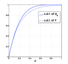
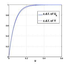
Figure 3: The c.d.f.’s $F_{U_{k}}$ and $F_{Y}$ where $Y\sim Exponential(K)$ are plotted for 3 $K=5$ and 3 $K=15$.

For the simplified model, the cost function (similar to (10)) when the system is in state $(w,b)$ at stage $1\leq k\leq K-1$ is,

$$g_{k}((w_{k},b_{k}),a_{k})=\left\{\begin{array}[]{ll}{U}_{k+1}&\mbox{ if }a_{k}=0\\ -\eta b_{k}&\mbox{ if }a_{k}=1\end{array}\right.$$ (17)

We observe that due to the i.i.d. inter-wake time assumption the cost function is not dependent on the value of $w_{k}$. Also we need not consider conditioning on $W_{k}=w_{k}$ unlike in the previous section since the p.d.f. of $U_{k+1}$ does not depend on $w_{k}$. Hence, the optimal policy for this model is going to be independent of $w_{k}$ for each $k$. So we simplify the state space by ignoring the values of $w_{k}$ for each $k$, i.e., the state space is $\mathcal{\bar{X}}=[0,1]\bigcup\{\psi\}$. Control space $\mathcal{C}$ and the other disturbance component ${Z_{k}}$ remain the same. Since the state space is different, we make a small change to the definition of policy $\pi$ by allowing $\mu_{k}^{\pi}:\mathcal{\bar{X}}\rightarrow\mathcal{C}$. The state transition and cost functions remain same as in the previous section with $(w,b)$ replaced by $b$. Let $\pi_{SF}(\eta)$ represent the optimal policy for this model.

Let $J_{k}(b)$ be the optimal cost to go at stage $k$ when the state is $b$. Then, for all $b\in[0,1]$,

$$J_{K}(b)=-\eta b$$ (18)

Next when the stage is $K-1$, for $b\in[0,1]$,

$$J_{K-1}(b) = \min\{-\eta b,\mathbb{E}_{K}\left[{U}_{K}+J_{K}(\max\{b,Z_{K}\})\right]\}$$ (19)

$$= \min\{-\eta b,\mathbb{E}_{K}\left[{U}_{K}-\eta\max\{b,Z_{K}\}\right]\}$$

$$= -\eta\max\{b,\beta_{1}(b)\}$$

where $\beta_{1}$ is a function, which for $b\in[0,1]$ is given by,

$$\beta_{1}(b) = \mathbb{E}_{K}[\max\{b,Z_{K}\}]-\frac{\mathbb{E}_{K}[{U}_{K}]}{\eta}$$ (20)

$$= \mathbb{E}_{K}[\max\{b,Z\}]-\frac{1}{\eta K}$$

Here we have made use of the fact that $\mathbb{E}_{K}[{U}_{K}]=\frac{1}{K}$ and $Z_{K}\sim Z$. The p.d.f. of $Z$ is given in (2). Evidently, at stage $K-1$, the optimal action is to stop and transmit the packet if $b\geq\beta_{1}(b)$ and to continue otherwise. The following results about $\beta_{1}(b)$ can easily be obtained, the proof of which we provide in Appendix.

Lemma 4

1. $\beta_{1}$ is continuous, increasing and convex in $b$.

2. If $\beta_{1}(0)<0$, then $\beta_{1}(b)<b$ for all $b\in[0,1]$.

3. If $\beta_{1}(0)\geq 0$, then there is a unique $\alpha_{\eta}$ such that $\beta_{1}(\alpha_{\eta})=\alpha_{\eta}$.

4. If $\beta_{1}(0)\geq 0$, then $\beta_{1}(b)<b$ for $b\in(\alpha_{\eta},1]$ and $\beta_{1}(b)>b$ for $b\in[0,\alpha_{\eta})$.

$\blacksquare$

If $\beta_{1}(0)<0$, then define $\alpha_{\eta}=0$. Otherwise $\alpha_{\eta}$ is defined by $\beta_{1}(\alpha_{\eta})=\alpha_{\eta}$. Then

$$\mu^{\pi_{SF}(\eta)}_{K-1}(b)=\left\{\begin{array}[]{ll}1\mbox{, if }b\geq\alpha_{\eta}\\ 0\mbox{, otherwise}\end{array}\right.$$

We proceed to evaluate $J_{K-2}$.

$$J_{K-2}(b) = \min\{-\eta b,\mathbb{E}_{K}[U_{K-1}+J_{K-1}(\max\{b,Z_{K-1}\})]\}$$ (21)

$$= \min\{-\eta b,\mathbb{E}_{K}[U_{K-1}-\eta\max\{b,Z_{K-1},\beta_{1}(\max\{b,Z_{K-1}\})\}]\}$$

$$= -\eta\max\{b,\beta_{2}(b)\}$$

where,

$$\beta_{2}(b) = \mathbb{E}_{K}[\max\{b,Z,\beta_{1}(\max\{b,Z\})\}]-\frac{1}{\eta K}$$ (22)

Lemma 5

$\beta_{2}(b)\geq\beta_{1}(b)$ for any $b\in[0,1]$. In particular, if $b\geq\alpha_{\eta}$ then $\beta_{2}(b)=\beta_{1}(b)$.

Proof:

The first part follows easily because $\mathbb{E}_{K}[\max\{b,Z\}]$ $\leq\mathbb{E}_{K}[\max\{b,Z,\beta_{1}(\max\{b,Z\})\}]$. Next, if $b\geq\alpha_{\eta}$ then from Lemma 4, $\max\{b,Z\}\geq\beta_{1}(\max\{b,Z\})$, so that $\max\{b,Z,\beta_{1}(\max\{b,Z\})\}=\max\{b,Z\}$. Therefore,

$$\beta_{2}(b) = \mathbb{E}_{K}[\max\{b,Z\}]-\frac{1}{\eta K}$$

∎

Lemma 6

For every $1\leq k\leq K-2$ the following holds,

$$J_{k}(b)=-\eta\max\{b,\beta_{K-k}(b)\}$$ (23)

where,

$$\beta_{K-k}(b) = \mathbb{E}_{K}[\max\{b,Z,\beta_{K-(k+1)}(\max\{b,Z\})\}]-\frac{1}{\eta K}$$

and has the property, $\beta_{K-k}(b)\geq\beta_{K-(k+1)}(b)$ for any $b\in[0,1]$. In particular, if $b\geq\alpha_{\eta}$ then $\beta_{K-k}(b)=\beta_{1}(b)$.

Proof:

Proof is along the lines used to obtain Equations (21), (22) and Lemma 5. ∎

Corollary 7

The policy $\pi_{SF}(\eta)$ is of the following form,
$\mu^{\pi_{SF}(\eta)}_{K}(b)=1$ and

$$\mu^{\pi_{SF}(\eta)}_{k}(b)=\left\{\begin{array}[]{ll}1&\mbox{ if }b\geq\alpha_{\eta}\\ 0&\mbox{ otherwise }\end{array}\right.$$ (24)

for $1\leq k\leq K-1$. $\blacksquare$

Remarks: The policy is a simple one-step-look-ahead rule where at each $k$ $(1\leq k\leq K-1)$ the policy compares the cost of stopping at $k$ ($C_{s}=-\eta b$) with the cost of continuing for one more step and then stopping at $k+1$ $(C_{c}=\frac{1}{K}-\eta\mathbb{E}_{K}[\max\{b,Z\}])$. The policy is to stop if $C_{s}\leq C_{c}$ (simplification yields, stop if $b\geq\alpha_{\eta}$), continue otherwise. The policy is to transmit to the first node which makes a progress of more than $\alpha_{\eta}$. If all the nodes, make progress of less than $\alpha_{\eta}$ then transmit to the node whose progress is maximum at the instant the last node wakes up.

VII Analytical Results

In this section we apply the policy $\pi_{SF}(\eta)$ obtained from the simplified model to the actual model and obtain expressions for average progress and average delay incurred by node $i$. First we need some more notation. We abuse the notation $\mathcal{S}_{i}$ by allowing $\mathcal{S}_{i}(z)=\{y:|y-x_{i}|\leq r_{c},|x_{N+1}-y|<L_{i}-z\}$. $\mathcal{S}_{i}(z)$ is the set of points that are closer to the sink than $x_{i}$ by atleast $z\in[0,1]$ (see Fig. 4). When $z=0$, we simply use $\mathcal{S}_{i}$ instead of $\mathcal{S}_{i}(0)$. Let $p_{z}=\frac{|\mathcal{S}_{i}(z)|}{|\mathcal{S}_{i}|}$, where $|\mathcal{S}_{i}(z)|$ denotes the area of the region $\mathcal{S}_{i}(z)$. $p_{z}$ is the conditional probability that a node falls in the region $\mathcal{S}_{i}(z)$ conditioned on the event that the node belongs to $\mathcal{S}_{i}$.

Figure 4: $x_{i}$ and $x_{N+1}$ are the locations of node $i$ and sink respectively. $L_{i}$ is the distance between them, $r_{c}$ is the communication radius. $\mathcal{S}_{i}(z)$ is the set of all points that are within the communication radius of node $i$ and are closer to sink than $i$ by atleast $z$. $\mathcal{S}_{i}(z)$ is the shaded region in the figure.

VII-A Average values for $\pi_{SF}(\eta)$

When using policy $\pi_{SF}(\eta)$, node $i$ transmits to the first node which makes a progress of more than $\alpha_{\eta}$. If there are $k\geq 1$ nodes in the region $\mathcal{S}_{i}(\alpha_{\eta})$, since the wake time of each of these is uniform on $[0,1]$ and independent of each other, the average time until the first one wakes up is $\frac{1}{k+1}$. If the region $\mathcal{S}_{i}(\alpha_{\eta})$ is empty, then node $i$ will wait for all the nodes in $\mathcal{S}_{i}$ to wake up and then transmit to the one which makes the maximum progress. In this case the average delay is $\frac{K}{K+1}$. Therefore,

$$\mathbb{E}_{K}[D^{\pi_{SF}(\eta)}] = \sum_{k=1}^{K}{K\choose k}p_{\alpha_{\eta}}^{k}(1-p_{\alpha_{\eta}})^{K-k}\frac{1}{k+1}+{(1-p_{\alpha_{\eta}})}^{K}\frac{K}{K+1}$$ (25)

The expression for average progress can be written as,

$$\mathbb{E}_{K}[Z^{\pi_{SF}(\eta)}] = \int_{0}^{1}\mathbb{P}_{K}(Z^{\pi_{SF}(\eta)}>z)dz$$ (26)

When $z\in[0,\alpha_{\eta}]$ then the event $(Z^{\pi_{SF}(\eta)}>z,N_{i}=K)$ is same as the event that at least one node makes a progress of more than $z$. Therefore for $z\in[0,\alpha_{\eta}]$,

$$\mathbb{P}_{K}(Z^{\pi_{SF}(\eta)}>z)=1-{(1-p_{z})}^{K}$$ (27)

When $z\in(\alpha_{\eta},1]$ then the event $(Z^{\pi_{SF}(\eta)}>z,N_{i}=K)$ is the same as the event that the region $\mathcal{S}_{i}(\alpha_{\eta})$ is non-empty and the node to wake up first in this region makes a progress of more than $z$, the probabilty of which is $\frac{p_{z}}{p_{\alpha_{\eta}}}$. Therefore for $z\in(\alpha_{\eta},1]$,

$$\mathbb{P}_{K}(Z^{\pi_{SF}(\eta)}>z)=\left(1-{(1-p_{\alpha_{\eta}})}^{K}\right)\frac{p_{z}}{p_{\alpha_{\eta}}}$$ (28)

VII-B Average Values for $\pi_{FF}$

The policy $\pi_{FF}$ (First Forward) transmits to the node in the region $\mathcal{S}_{i}$ which wakes up first, irrespective of the progress made by it. Therefore,

$$\mathbb{E}_{K}[D^{\pi_{FF}}] = \frac{1}{K+1}$$ (29)

Average progress is,

$$\mathbb{E}_{K}[Z^{\pi_{FF}}] = \int_{0}^{1}\mathbb{P}_{K}(Z^{\pi_{FF}}>z)dz$$ (30)

$$= \int_{0}^{1}p_{z}dz$$

VII-C Average Values for $\pi_{MF}$

The policy $\pi_{MF}$ (Max Forward) always waits for all the nodes to wake up and then transmits to the node which makes the maximum progress. Therefore,

$$\mathbb{E}_{K}[D^{\pi_{MF}}] = \frac{K}{K+1}$$ (31)

Average progress is given by,

$$\mathbb{E}_{K}[Z^{\pi_{MF}}] = \int_{0}^{1}\mathbb{P}_{K}(Z^{\pi_{MF}}>z)dz$$ (32)

$$= \int_{0}^{1}\left(1-{(1-p_{z})}^{K}\right)dz$$

VIII Simulation Results

VIII-A One Hop Performance

We apply the policies $\pi_{BF}(\eta)$ and $\pi_{SF}(\eta)$ to the actual model and obtain average progress and average one hop delay for $L_{i}=10$ and $K=5$. Expressions for the average values for policies $\pi_{SF}(\eta)$, $\pi_{FF}$ and $\pi_{MF}$ were obtained in Section VII. Since it is difficult to obtain similar analytical expressions for policy $\pi_{BF}(\eta)$, we have performed simulations to obtain these values. In Figs. 5 and 5 we plot the average values as a function of $\eta$. The minimum and maximum values of average delay and progress are achieved by $\pi_{FF}$ and $\pi_{MF}$ respectively. From the figures we can observe that for values of $\eta$ less than $\eta_{o}=\frac{1}{\mathbb{E}_{K}[Z]K}$ the performance of $\pi_{SF}(\eta)$ is same as $\pi_{FF}$. This is because for $\eta$ less than $\eta_{o}$, we have $\beta_{1}(0)<0$, and therefore the threshold used is $\alpha_{\eta}=0$ which is same as that used by $\pi_{FF}$.

By using a large value of $\eta$, a node will value progress more and will end up waiting for better nodes to wake up thus incurring a large delay as well. Hence, delay and progress for both the policies ($\pi_{BF}$ and $\pi_{SF}$) are increasing with $\eta$. We can conclude from Lemma 1, that for each policy, BF or SF, and a given $\eta$, the corresponding delay value is the minimum that can be obtained using that policy, subject to a constraint on progress equal to the progress value obtained for that $\eta$. These corresponding average delay vs. average progress values are shown in Fig. 5, for $K=3,5$ and $15$. Each point on the curve for each $K$ corresponds to a different value of $\eta$, which increases along the curves as shown. We see that the performance of the $SF$ policy is close to that of the optimal BF policy, even for small values of $K$. The way $\eta$ serves to trade-off one hop progress and delay is clearly shown by these curves.

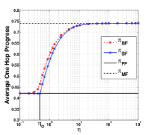
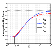
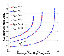
Figure 5: One Hop Performance: 5: Average one hop progress as a function of $\eta$ for various policies. The plots are for $L_{i}=10$ and $K=5$. Maximum and minimum progress are achieved by $\pi_{MF}$ and $\pi_{FF}$ respectively. 5: Average one hop delay as a function of $\eta$ for various policies. The plots are for $L_{i}=10$ and $K=5$. Maximum and minimum delay are achieved by $\pi_{MF}$ and $\pi_{FF}$. 5: Average one hop delay vs. the corresponding average one hop progress for the class of policies $\pi_{BF}$ and $\pi_{SF}$ are plotted for $K=3,5$ and $15$. The parameter $\eta$ controls the delay-progress trade-off. Each point on the curve corresponds to a different value of $\eta$ which increases along the direction shown.

VIII-B End to End Performance

Although our policies have been developed for one-hop optimality, it is interesting to study their end-to-end performance if they were used, heuristically, at each hop. We compare the end-to-end performance of our policy with the work of Kim et al. [1] who have developed end-to-end delay optimal geographical forwarding in a setting similar to ours. We first give a brief description of their work. They minimize, for a given network, the average delay from any node to the sink when each node $i$ wakes up asynchronously with rate $r_{i}$. They show that periodic wake up patterns obtain minimum delay among all sleep-wake patterns with the same rate. A relay node with a packet to forward, transmits a sequence of beacon-ID signals. They propose an algorithm called LOCAL-OPT [17] which yields, for each neighbor $j$ of node $i$, an integer $h_{j}^{(i)}$ such that if $j$ wakes up and listens to the $h-th$ beacon signal from node $i$ and if $h\leq h_{j}^{(i)}$, then $j$ will send an ACK to receive the packet from $i$. Otherwise (if $h>h_{j}^{(i)}$) $j$ will go back to sleep. A configuration phase is required to run the LOCAL-OPT algorithm.

As before, we fix $r_{c}=1$ and $T=1$ sec. Each node wakes up periodically with rate $\frac{1}{T}$ but asynchronously. To make a fair comparision with the work of Kim et al. we introduce beacon-ID signals of duration $t_{I}=5$ msec and packet transmission duration of $t_{D}=30$ msec. We fix a network by placing $N$ nodes randomly in $[0,L]^{2}$ where $L=10$. $N$ is sampled from Poisson($\lambda L^{2}$) where $\lambda=5$. Additional source and sink nodes are placed at locations $(0,0)$ and $(L,L)$ respectively. Further we have considered a network where the forwarding set of each node is non-empty. The wake times of the nodes are sampled independently from Uniform([0,1]). Description of the policies that we have implemented is given below.

$\pi_{SF}$: We fix $\gamma$ as a network parameter. Each relay node chooses an appropriate $\eta$ (in other words, chooses an appropriate threshold $\alpha_{\eta}$) such that the average one hop progress made using the policy $\pi_{SF}(\eta)$ is equal to $\gamma$. Note that ${\eta}$ depends on node $i$ (i.e., on the values of $L_{i}$ and $K$). At a relay node $i$ if $\gamma$ is less (greater) than the average progress made by $\pi_{FF}$ ($\pi_{MF}$) then we allow node $i$ to use $\pi_{FF}$ ($\pi_{MF}$) to forward. When a node $j$ wakes up and if it hears a beacon signal from $i$, it waits for the ID signal and then sends an ACK signal containing its location information. If the progress made by $j$ is more than the threshold, then $i$ forwards the packet to $j$ (packet duration is $t_{D}=30$ msec). If the progress made by $j$ is less than the threshold, then $i$ asks $j$ to stay awake if its progress is the maximum among all the nodes that have woken up thus far, otherwise $i$ asks $j$ to return to sleep. If more than one node wakes up during the same beacon signal, then contentions are resolved by selecting the one which makes the most progress among them. In the simulation, this happens instantly (as also for the Kim et al. algorithm that we compare with); in practice this will require a splitting algorithm; see, for example, [18, Chapter 4.3]. We assume that within $t_{I}=5$ msec all these transactions (beacon signal, ID, ACK and contention resolution if any) are over. $\pi_{FF}$ and $\pi_{MF}$ can be thought of as special cases of $\pi_{SF}$ with thresholds of $0$ and $1$ respectively.

$\hat{\pi}_{SF}$: This is same as $\pi_{SF}$ except that here a relay node does not know $K$, but estimates its value as $\lfloor\lambda|\mathcal{S}_{i}|\rfloor$ nodes where $|\mathcal{S}_{i}|$ is the area of the region $\mathcal{S}_{i}$ (Equation (3)). If there is no eligible node even after the $\frac{T}{t_{I}}-th$ beacon signal (one case when this is possible is when the actual number of nodes $K$ is less than $\lfloor\lambda|\mathcal{S}_{i}|\rfloor$ and none of the nodes make a progress of more than the threshold) then $i$ will select one which makes the maximum progress among all nodes.

Kim et al.: We run the LOCAL-OPT algorithm [17] on the network and obtain the values $h_{j}^{(i)}$ for each pair $(i,j)$ where $i$ and $j$ are neighbors. We use these values to route from source to sink in the presence of sleep wake cycling. Contentions, if any, are resolved (instantly, in the simulation) by selecting a node $j$ with the highest $h_{j}^{(i)}$ index.

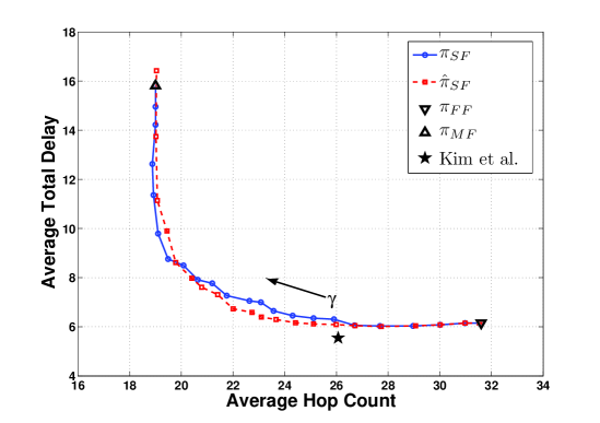
Figure 6: End-to-end performance: Plot of average end-to-end delay vs. average end-to-end hop count when the one hop optimal policy for the progress constraint $\gamma$ is used at each hop. The operating points of the policies $\pi_{FF}$, $\pi_{MF}$ and Kim et al. are also shown in the figure. Each point on the curve corresponds to a different value of $\gamma$ which increases along the direction shown.

In Fig. 6 we plot average total delay vs. average hop count for different policies for fixed node placement, while the averaging is over the wake times of the nodes. Each point on the curve is obtained by averaging over 1000 transfers of the packet from the source node to the sink. As expected, Kim et al. achieves minimum average delay. In comparision with $\pi_{FF}$, Kim et al. also achieves smaller average hop count. Notice, however that using $\pi_{SF}$ policy and properly choosing $\gamma$, it is possible to obtain hop count similar to that of Kim et al., incurring only slightly higher delay.

The advantage of $\pi_{SF}$ over Kim et al. is that there is no need for a configuration phase. Each relay node has to only compute a threshold that depends on the parameter $\gamma$ which can be set as a network parameter during deployment. A more interesting approach would be to allow the source node to set $\gamma$ depending on the type of application. For delay sensitive applications it is appropriate to use a smaller value of $\gamma$ so that the delay is small, whereas, for energy constrained applications (where the network energy needs to conserved) it is better to use large $\gamma$ so that the number of hops (and hence the number of transmissions) is reduced. For other applications, moderate values of $\gamma$ can be used. $\gamma$ can be a part of the ID signal so that it is made available to the next hop relay.

Another interesting observation from Fig. 6 is that the performance of $\hat{\pi}_{SF}$ is close to that of $\pi_{SF}$. In practice it might not be reasonable to expect a node to know the exact number of relays in the forwarding set. $\hat{\pi}_{SF}$ works with average number of nodes instead of the actual number. For small values of $\gamma$ both the policies $\pi_{SF}$ and $\hat{\pi}_{SF}$, most of the time, transmit to the first node to wake up. Hence the performance is similar for small $\gamma$. For larger $\gamma$, we observe that the delay incurred by $\hat{\pi}_{SF}$ is larger.

IX Summary and Future Work

The problem of optimal relay selection for geographical forwarding was formulated as one of minimizing the forwarding delay subject to a constraint on progress. The simple policy (SF) of transmitting to the first node that wakes up and makes a progress of more than a threshold was found to be close in performance to the optimal policy. We then compared the end-to-end performance (average delay and average hop count) of using SF at each relay node enroute to the sink with that of the policy proposed by Kim et al. [1], which is designed to achieve minimum average end-to-end delay. However, the delay obtained by the policy in [1] is only a little smaller than that obtained by the FF policy. Further, by using the SF policy with a appropriate $\gamma$, performance very close to that of the policy in [1] can be obtained without the need for an initial global configuration phase. We note that $\pi_{SF}$ is self-configuring; each node takes decisions based only on local information. The end-to-end performance obtained can be tuned by the use of a single parameter $\gamma$. For a small $\gamma$ we obtain low end-to-end delay but the number of hops is large and vice versa.

In this work we have assumed that each node knows the number of neighbors in its forwarding set. We had given a heuristic policy $\hat{\pi}_{SF}$ when the actual number of forwarding neighbors is not known. In future work we aim to obtain optimal forwarding policies by relaxing this assumption. Also, the use of a one-hop optimal policy for end-to-end forwarding is a heuristic. In future work we propose to directly formulate the end-to-end problem and derive optimal policies. In addition, we could also include aspects such as the relay’s link quality in our formulation.

[Proof of Lemma 4]

Proof:

Recall from Equation (20) that

$$\beta_{1}(b) = \mathbb{E}_{K}[\max\{b,Z\}]-\frac{1}{\eta K}$$

Let $F_{Z}$ represent the $c.d.f.$ of $Z$. For $b\in[0,1]$, the $c.d.f.$ of $\max\{b,Z\}$ is,

$$F_{\max\{b,Z\}}(z)=\left\{\begin{array}[]{ll}0&\mbox{ if }z<b\\ F_{Z}(z)&\mbox{ if }z\geq b\end{array}\right.$$

$$\beta_{1}(b) = \int_{0}^{1}(1-F_{\max\{b,Z\}}(z))dz-\frac{1}{\eta K}$$

$$= b+\int_{b}^{1}(1-F_{Z}(z))dz-\frac{1}{\eta K}$$

${\beta_{1}}^{\prime}(b)=F_{Z}(b)\geq 0$ and ${\beta_{1}}^{\prime\prime}(b)=f_{Z}(b)\geq 0$ implies that $\beta_{1}$ is continuous, increasing and convex in $b$. ∎

Proof:

Since $\mathbb{E}_{K}[\max\{b,Z\}]\leq 1$, $\eta>0$ and $K>0$, we have $\beta_{1}(1)<1$. Also $\beta_{1}$ is convex (from Lemma 4.1). Hence we can write,

$$\beta_{1}(b) \leq (1-b)\beta_{1}(0)+b\beta_{1}(1)$$

$$< b$$

∎

Proof:

Let $g(b)=b-\beta_{1}(b)$. Then, $g(0)\leq 0$ and $g(1)>0$ (because $\beta_{1}(1)<1$). Also $g(b)$ is continuous (being differentiable) on $[0,1]$. Hence, $\exists$ an $\alpha_{\eta}\in[0,1)$ such that $g(\alpha_{\eta})=0$.

Suppose $\exists$ an ${\alpha}^{\prime}_{\eta}>{\alpha_{\eta}}$ such that $g({\alpha}^{\prime}_{\eta})=0$. Then by convexity of $\beta_{1}$ (from Lemma 4.1),

$$\beta_{1}({\alpha}^{\prime}_{\eta}) \leq \frac{1-{\alpha}^{\prime}_{\eta}}{1-{\alpha_{\eta}}}\beta_{1}(\alpha_{\eta})+\frac{{\alpha}^{\prime}_{\eta}-{\alpha_{\eta}}}{1-{\alpha_{\eta}}}\beta_{1}(1)$$

$i.e.,$ ${\beta_{1}}(1)\geq 1$. Contradicts the fact that, $\beta_{1}(1)<1$. ∎

Proof:

Again consider $g(b)=b-\beta_{1}(b)$. $g(b)$ is continuous (being differentiable) on $[0,1]$. Suppose $\exists$ $b\in(\alpha_{\eta},1]$ such that $\beta_{1}(b)>b$, then $g(b)\leq 0$ and $g(1)>0$. This implies that $\exists$ $b^{\prime}$ in $[b,1)$ such that $g(b^{\prime})=0$. Contradicts the uniqueness of $\alpha_{\eta}$ shown in Lemma 4.3. Similarly it can be shown that $\beta_{1}(b)>b$ for $b\in[0,\alpha_{\eta})$. ∎

References

- [1] J. Kim, X. Lin, and N. Shroff, “Optimal Anycast Technique for Delay-Sensitive Energy-Constrained Asynchronous Sensor Networks,” in INFOCOM 2009. The 28th Conference on Computer Communications. IEEE, April 2009, pp. 612–620.
- [2] H. Takagi and L. Kleinrock, “Optimal Transmission Ranges for Randomly Distributed Packet Radio Terminals,” Communications, IEEE Transactions on [legacy, pre - 1988], vol. 32, no. 3, pp. 246–257, 1984.
- [3] T. C. Hou and V. Li, “Transmission Range Control in Multihop Packet Radio Networks,” Communications, IEEE Transactions, vol. 34, no. 1, pp. 38–44, 1986.
- [4] B. Karp and H. T. Kung, “GPSR: Greedy Perimeter Stateless Routing for Wireless Networks,” in MobiCom ’00: Proceedings of the 6th annual international conference on Mobile computing and networking. New York, NY, USA: ACM Press, 2000, pp. 243–254.
- [5] F. Kuhn, R. Wattenhofer, and A. Zollinger, “An Algorithmic Approach to Geographic Routing in Ad Hoc and Sensor Networks,” IEEE/ACM Trans. Netw., vol. 16, no. 1, pp. 51–62, 2008.
- [6] S. Dulman, M. Rossi, P. Havinga, and M. Zorzi, “On the Hop Count Statistics for Randomly Deployed Wireless Sensor Networks,” Int. J. Sen. Netw., vol. 1, no. 1/2, pp. 89–102, 2006.
- [7] S. Nath and A. Kumar, “Performance Evaluation of Distance Hop Proportionality on Geometric Graph Models of Dense Sensor Networks,” Proc. 3rd International Conference on Performance Evaluation Methodologies and Tools (Valuetools ’08), Athens, Greece, October 2008.
- [8] M. Mauve, J. Widmer, and H. Hartenstein, “A Survey on Position-Based Routing in Mobile Ad-Hoc Networks,” IEEE Network, vol. 15, pp. 30–39, 2001.
- [9] K. Akkaya and M. Younis, “A Survey on Routing Protocols for Wireless Sensor Networks,” Ad Hoc Networks, vol. 3, pp. 325–349, 2005.
- [10] V. Paruchuri, S. Basavaraju, A. Durresi, R. Kannan, and S. S. Iyengar, “Random Asynchronous Wakeup Protocol for Sensor Networks,” Broadband Networks, International Conference on, vol. 0, pp. 710–717, 2004.
- [11] S. Liu, K. W. Fan, and P. Sinha, “CMAC: An Energy Efficient MAC Layer Protocol using Convergent Packet Forwarding for Wireless Sensor Networks,” in Sensor, Mesh and Ad Hoc Communications and Networks, 2007. SECON ’07. 4th Annual IEEE Communications Society Conference on, June 2007, pp. 11–20.
- [12] M. Zorzi, S. Member, R. R. Rao, and S. Member, “Geographic Random Forwarding (GeRaF) for Ad Hoc and Sensor Networks: Multihop Performance,” IEEE Transactions on Mobile Computing, vol. 2, pp. 337–348, 2003.
- [13] M. Rossi, M. Zorzi, and R. R. Rao, “Statistically Assisted Routing Algorithms (SARA) for Hop Count Based Forwarding in Wireless Sensor Networks,” Wirel. Netw., vol. 14, no. 1, pp. 55–70, 2008.
- [14] P. Chaporkar and A. Proutiere, “Optimal Joint Probing and Transmission Strategy for Maximizing Throughput in Wireless Systems,” Selected Areas in Communications, IEEE Journal on, vol. 26, no. 8, pp. 1546–1555, October 2008.
- [15] H. A. David and H. N. Nagaraja, Order Statistics (Wiley Series in Probability and Statistics). Wiley-Interscience, August 2003.
- [16] D. P. Bertsekas, Dynamic Programming and Optimal Control, Vol. I. Athena Scientific, 2005.
- [17] J. Kim, X. Lin, and N. B. Shroff, “Optimal Anycast Technique for Delay Sensitive Energy-Constrained Asynchronous Sensor Networks,” 2008, Technical Report, Purdue University. [Online]. Available: http://web.ics.purdue.edu/~kim309/Kim08tech3.pdf
- [18] D. Bertsekas and R. Gallager, Data networks. Upper Saddle River, NJ, USA: Prentice-Hall, Inc., 1992.