A Near-Infrared Study of the Stellar Cluster: [DBS2003] 45

Abstract

We present a multi-wavelength photometric and spectroscopic study of a newly discovered candidate cluster [DBS2003] 45. Our H, Ks photometry confirms that [DBS2003] 45 is a cluster. An average visual extinction A_V$\sim$7.1$\pm$0.5 is needed to fit the cluster sequence with a model isochrone. Low resolution spectroscopy indicates that half a dozen early B and at least one late O type giant stars are present in the cluster. We estimate the age of the cluster to be between 5 and 8 Myr based on spectroscopic analysis. Assuming an age of 6 Myr, we fit the observed mass function with a power law, N(M) $\varpropto$ M^-Γ, and find an index $\Gamma\sim$ 1.27$\pm$0.15, which is consistent with the Salpeter value. We estimate the total cluster mass is around 10³M_⊙ by integrating the derived mass function between 0.5 and 45 M_⊙. Both mid-infrared and radio wavelength observations show that a bubble filled with ionized gas is associated with the cluster. The total ionizing photon flux estimated from radio continuum measurements is consistent with the number of hot stars we detected. Infrared bright point sources along the rim of the bubble suggest that there is triggered star formation at the periphery of the HII region.

1 Introduction

Stellar clusters serve as ideal laboratories to study the evolution of stars of different masses, as the stars in a cluster are formed at the same time from the same molecular cloud. This assumption predicts that the stars are at the same distance, have practically the same initial chemical abundances, and evolve in a similar physical environment. Such a coeval population can be used to make critical tests of theoretical stellar evolution models. Young clusters are of particular interest for this purpose because most of their massive stellar members are still in main sequence (MS) or post-MS stages before supernova explosions. Studies of such stars can improve our understanding about the formation and evolution of massive stars, as well as the evolution of whole clusters in general.

Stars generally form with a frequency that decreases with increasing mass for M$>$1 M_⊙, i.e. $\Gamma$=d(log N)/d(log m) $\sim$ -1.35 (Salpeter, 1955; Scalo, 1998; Kroupa, 2001, 2002). This initial mass function (IMF) has been used extensively. However, some evidence suggests that the function may not be universal. Figer et al. (1999), Stolte et al. (2002) and Kim et al. (2006) claim a significantly shallower slope for the Arches cluster. This result, for one of the most massive and the densest cluster in the Galaxy, suggests that more massive and dense clusters have a shallow IMF. Alternatively, perhaps the Galactic center favors shallow IMFs (Morris, 1993). Since the existing IMF slope of -1.35 was first measured by Salpeter (1955) for field stars with masses lower than 10 M_⊙ and field stars have a MF which is different from the IMF of clusters, the claim of a universal IMF seems questionable. Zinnecker & Yorke (2007) commented that, although massive stars can form locally in the field, evidence suggested that massive stars form preferentially in dense clusters or OB associations. Additionally, mass segregation can cause massive stars to sink toward the cluster center and the cluster continuously loses low mass stars to the field. These effects would modify the cluster MF so that it becomes shallower as the age of the cluster increases. The ultimate resolution to this question will come from measurements of the IMF in stellar clusters throughout the Galaxy. The sample of newly-identified clusters provides a fresh opportunity for this purpose.

There are less than 1600 open clusters discovered at optical wavelengths in our galaxy (Dias et al., 2002). It is reasonable to believe that a large number of such clusters are missed by optical observations due to substantial line-of-sight interstellar extinction in the Galactic plane. The advance of infrared technology allows surveys to be carried out in near infrared (NIR) and mid infrared (mid-IR) wavelengths to circumvent the problem of high extinction. Systematic searches for Galactic open cluster candidates have been carried out in infrared bands and more than 1000 new candidates were discovered (Bica et al., 2003; Dutra et al., 2003a, b; Froebrich et al., 2007), although many of them remain unconfirmed and extensive efforts in follow-up observations are needed to determine their true identities..

Here we present our photometric and spectroscopic analysis of [DBS2003] 45, a candidate cluster chosen from such an infrared cluster catalog (Dutra et al., 2003a). This target is located at (l, b) = (283.^∘88, -0.^∘91) and is about 3.5 degrees on the sky to the west of the Carina nebula (NGC3372), suggesting that the candidate cluster is likely located in the Sagittarius-Carina spiral arm. In § 2, we describe the origin of data that are used in this work. Our data reduction procedure is described in § 3. In § 4, we present the results of our analysis. Some issues related to our observation are discussed in § 5. Finally, we summarize our findings in § 6.

2 Observations

Photometric observations of [DBS2003] 45 were carried out on the ESO 3.8m New Technology Telescope (NTT) with SofI in 2008 February (ESO proposal ID 080.D-0470 ). SofI is an infrared spectrograph and imaging camera equipped with a Rockwell Hg:Cd:Te 1024 $\times$ 1024 HAWAII array of 18.5 micron pixel-size (Moorwood et al., 1998). It takes images with a plate scale of 0.288^′′/pixel. H and Ks band images of the target field were obtained in a dither pattern in which candidate clusters were shifted to one of four corners of the detector each time. We used discrete integration times (DITs) of 2s, coadded 10 times, in 4 dithers. Multiple images were taken at each dither location, resulting in a total 160s of integration time for the location of the cluster at each waveband.

We also obtained low-resolution spectroscopy of several stars in the field of the cluster. We used the ‘Red’ grism in conjunction with the 0.6″ slit, giving a spectral resolution of $R\sim 900$ in the wavelength range 1.9 - 2.4$\mu$m. We employed DITs of 40-60s, repeated twice at each position. After each integration the target was nodded 20″ along the slit. Each object was observed in 8 nod positions, hence total integration times were 16mins per object. For fainter objects ($Ks>10$) we increased the number of nod positions to 16 in order to improve signal-to-noise. To correct for atmospheric absorption, the solar-type star Hip059532 was observed immediately after observing the cluster stars. Dark-frames and flat-field observations were made during twilight. For wavelength calibration purposes a neon arc lamp was observed.

Additionally, images of the field were taken in four bands at 3.6, 4.5, 5.8, and 8 $\mu$m on February 2007 using the infrared camera - IRAC on the Spitzer space telescope (Program ID: 30734). During the observations, we used the 5 position Gaussian dithering pattern. The resulting images of each band cover an area of 5^′ by 5^′ with a pixel size of 1.2^′′ in both directions of RA and DEC. The total integration time on target is 471s.

In order to study the nebulosity surrounding the cluster and its association with the cluster, we use H_α, mid-infrared maps, and radio survey data. H_α line observations were taken from superCOSMOS survey archive (Parker et al., 2005). Radio flux is obtained from Parkes-MIT-NRAO 4850 MHz southern sky survey catalog (Wright et al., 1994). We also obtained from the archive an 8 $\mu$m image of a large area including our field taken by Spitzer/IRAC (Program ID: 40791). The mid-IR image and the H_α emission map will be compared in order to address the association between the cluster and the bubble.

3 Data Reduction and Analysis

Our photometric and spectroscopic data sets come from different sources. Therefore, the reduction procedure is slightly different for individual data set. The SofI data set includes both photometric and spectroscopic observations. Here we describe their reduction procedures separately.

3.1 SofI Data

3.1.1 Photometry

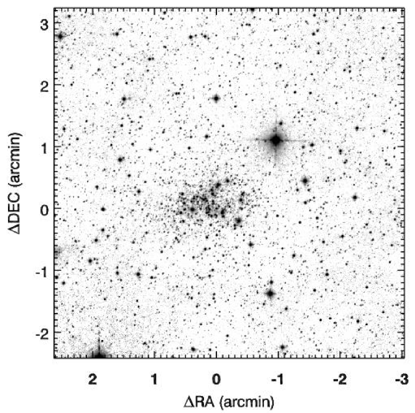
Figure 1: Ks band mosaic of the cluster candidate [DBS2003] 45 in a logarithmic scale. The origin of the axes corresponds to R.A.=10^h19^m10.5^s, Decl.=-58^∘02^′22.6^′′ (2000).

Our SofI photometric data consists of two bands, H and Ks, with eight partially overlapping images in each band. The flat-fielding is done using facility provided dark and flat frames. A group of 8 images that were obtained closest in time are scaled according to the integration time and median-combined to create a sky background image. This background image is scaled and subtracted from each flat-fielded image of the target. The resulting images are re-sampled, cross-correlated, shifted, and coadded to create a mosaic. We register resulting mosaics with downloaded 2MASS mosaics of the same field in the same photometrical bands to correct for astrometric errors in our observations. We manually pick a group of relatively bright and isolated stars that can be seen in both SofI and 2MASS mosaics. Using the 2MASS coordinates of these bright stars, we compute the geometric transformation coefficients between the coordinates of observed images and the 2MASS images. The observed images are re-mapped onto the 2MASS grid to produce the final images for photometric analysis. The final Ks band image is shown in Figure 1.

3.1.2 Calibration

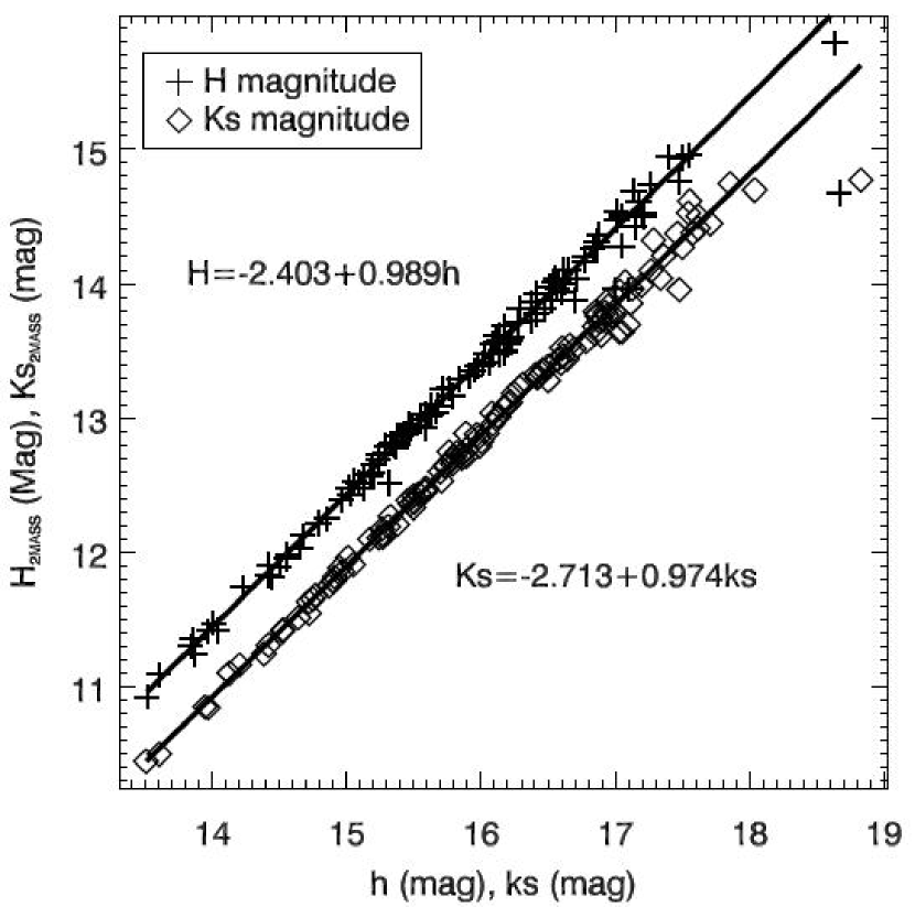
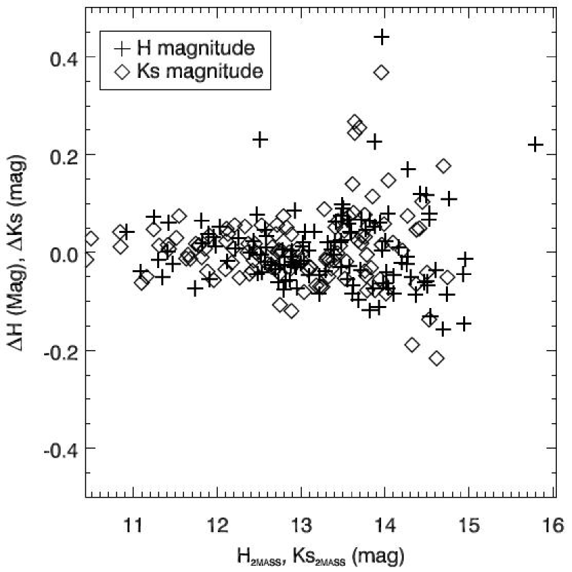
Figure 2: Using 2MASS magnitudes to calibrate the observed photometry. In both figures, plus signs indicate H band magnitudes and diamonds in the figures indicate Ks band magnitudes. In the left figure, x and y axes are observed and 2MASS magnitudes, respectively. Solid lines and equations show the results of a single variable linear model fitting. In the right figure, x axis is the calibrated magnitude and y axis is the difference between the calibrated and the instrumental magnitudes.

The aperture photometry of point sources are obtained for the SofI data using an IDL adapted version of the DAOPHOT. Since all images are re-mapped onto the 2MASS grid, the magnitudes of different bands can be associated using stellar locations. The same group of stars that were used to register the SofI mosaics are used to calibrate detected H and Ks band magnitudes. Figure 2(left) shows corresponding instrumental and 2MASS magnitudes of these stars with plus signs and diamonds representing H and Ks band magnitudes, respectively. It clearly shows that linear relations (solid lines) exist between two sets of measurements.

To account for any color term effect present in the data, the following linear bivariate model between the instrumental magnitudes and the 2MASS magnitudes is assumed:

$$h = a_{h}+b_{h}H+c_{h}Ks$$ (1)

$$ks = a_{k}+b_{k}H+c_{k}Ks$$ (2)

here, h and ks are instrumental magnitudes of the picked stars. H and Ks are the corresponding 2MASS magnitudes. The model coefficients are determined using a regression method. Once all coefficients have been determined, the following equations are used to compute calibrated magnitudes of all stars in the field

$$H = \frac{c_{k}h-c_{h}ks-a_{h}c_{k}+a_{k}c_{h}}{b_{h}c_{k}-c_{h}b_{k}}$$ (3)

$$Ks = \frac{b_{k}h-b_{h}ks-a_{h}b_{k}+a_{k}b_{h}}{c_{h}b_{k}-b_{h}c_{k}}$$ (4)

or

$$H = A_{H}+B_{H}h+C_{H}ks$$ (5)

$$Ks = A_{K}+B_{K}h+C_{K}ks$$ (6)

here, coefficients in the capital form (A, B, C) are the results of combining the corresponding terms in the equation 3. Table 1 shows the coefficients found by our regression procedure and indicates small amount of color effect. Figure 2 (right) shows the corrections between instrumental and calibrated magnitudes. Again, diamonds and plus signs in the figure indicate Ks and H band magnitudes, respectively.

3.1.3 Completeness Test

The ability to detect stars is impaired when dealing with crowded fields. Faint stars are likely missed by a star finding procedure due to the overlapping of stellar point spread functions (PSFs). A completeness test is carried out to correct for such an error and to establish the actual magnitude distribution. We add artificial stars to the mosaics and apply the same star extracting procedure to see whether or not they can be recovered. Stars detected in each mosaic are ranked based on their distances from neighboring stars. The first 20 unsaturated stars with the largest separations are picked. Each star’s PSF is extracted from the mosaic and the local sky background is subtracted. Finally, the individual PSFs are re-sampled, shifted, and added to create a template PSF.

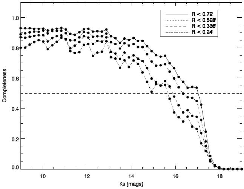
Figure 3: The completeness curves of the derived photometry for the candidate cluster when choosing different sizes. The curve for the outermost region shows that the photometry is 50% complete at Ks$\simeq$17. The dashed line indicates 50% completeness.

We divide the magnitude range from 9 to 19 magnitudes into bins with a binsize of 1 magnitude. Within each bin, we create 50 fake stars with their magnitudes uniformly distributed across the bin. The images of the stars are created by scaling the template PSF and added to the input mosaic at random locations within 43^′′ from the center of the cluster field. The resulting mosaic is then treated with DAOPHOT in the exactly same manner that is used to find stars in the original extraction. If a star is found at the location where a fake star is added and the difference between the input and output magnitudes is less than 0.5 mag, we define that the fake star is recovered. Otherwise, we define that the added artificial star is missing. We repeat this experiment 10 times and generate 500 artificial stars total which are evenly distributed over the magnitude bins. Figure 3 shows the curve of completeness from our simulation, which suggests that we achieve the 50% completeness at M${}_{Ks}{\simeq}$17 (mag) at the center of the field.

3.1.4 Spectroscopy

We first subtracted dark frame from each science frame to minimize fixed-pattern noise of the detector. Observations at two complimentary nod-positions were then subtracted from each other to remove atmospheric OH emission lines. Repeating observations were averaged to reduce noise. Afterwards, spectra were extracted from the average frame by summing the rows across the width of the spectral traces. A spectrum of the arc lamp at the same position on the chip was also extracted using the same extraction procedure. Wavelength calibration was achieved by fitting the locations of the arc lines with a 4th-degree polynomial. Atmospheric absorption in the stellar spectra was removed using the telluric standard star, which had first been divided through by a synthetic spectrum of a GV star. Finally, stellar spectra were normalized by dividing through by their median continuum values. The reduced spectra are shown in Figure 4. The coordinates of the stars are listed in Table 2. From flat regions of continuum, we estimate the signal-to-noise of the spectra are 80 or better.

3.2 Spitzer IRAC Photometry

The basic calibrated data (bcd) was downloaded and used to create new mosaics using Spitzer’s Mopex tool before the mosaics were treated with DAOPHOT. Point spread function (psf) photometry was performed in order to achieve deeper photometric detection. After every round of star finding process, the detected stars were subtracted from the mosaic to create a residual mosaic. Additional rounds of star finding were then performed on the resulting mosaics until no additional stars were found in the final image. Finally, all detected point sources were collected and cross-correlated with 2MASS point sources for completeness.

4 Results

4.1 Color Magnitude Diagram

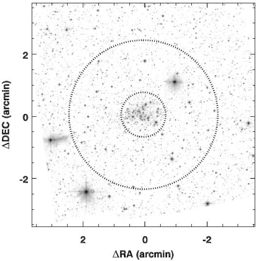
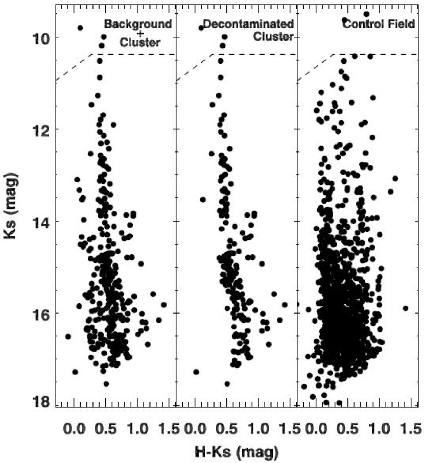
Figure 5: The Color-Magnitude diagram (CMD) of [DBS2003] 45. The Ks band image (in a logarithmic scale) on the left shows the region from which the CMDs are drawn. Two concentric circles centered at (RA, DEC) = (10^h19^m10.5^s, -58^∘02^′22.6^′′) demonstrate the central circular region and an annulus region chosen for the cluster candidate and the control field. The radii of the circles are 0.72 and 2.4 arcmin, respectively. The CMDs on the right in the figure are for the cluster with background contamination (left panel), the decontaminated cluster (middle panel) and the control field CMD (right panel), respectively.

Figure 5(right) shows color magnitude diagrams (CMDs) of the candidate cluster before (left panel) and after (middle panel) field contamination has been removed and the CMD of a chosen control field (right panel) for our SofI data. The image on the left demonstrates how the regions for the cluster and the control field are defined. A circular region with a radius $\sim$0.72 arcmin is chosen for the cluster and it includes the densest part of the observed field. An annulus region outside the circular region is chosen as the control field, which has an outer radius about 2.4 arcmin. Both regions are centered at RA(2000)=10^h19^m10.5^s, Dec(2000)=-58^∘02^′22.6^′′. The CMD of the control field is scaled based on the area ratio of regions for the cluster and the field and is subtracted from the CMD of the cluster+field. The resulting decontaminated cluster CMD is shown in the middle panel of Figure 5(right), which demonstrates clearly a cluster sequence with majority of stars along a vertical line with H-Ks$\simeq$0.45. Among 175 remaining stars, the brightest one has Ks$\simeq$10. Since a few stars are located above our saturation limit (dashed lines in the CMDs), we have replaced presumably saturated magnitudes with the corresponding values in the 2MASS catalog, which does not significantly change the locations of those stars on our CMDs.

4.2 Spectroscopy

Low-resolution spectra of a few relatively bright stars present in the field of the candidate cluster are shown in the right panel of Figure 4 with their locations indicated in a Ks band image of the field on the left together with other stars remaining in the cluster CMD. The spectrum of the brightest star in the field #8 shows CO bandhead absorption. The CO equivalent width is consistent with the star being either a late-type giant (M5-7III) or a supergiant of an earlier type (K2-4 I). The spectrum of the star #6 shows faint emission at the wavelengths of the Br$\gamma$ line and the HeI 2.06 $\mu$m line and absorption in the HeI 2.11 $\mu$m line. All other spectra show weak absorption at the wavelengths of the Br$\gamma$ line, the 2.06 $\mu$m and 2.11 $\mu$m HeI lines. None of these spectra shows significant contribution from the 2.19 $\mu$m HeII line.

According to the atlas provided by Hanson et al. (2005), stars earlier than O9.5 usually show HeII 2.19 $\mu$m line in absorption in their spectra. This feature should be as strong as the Br$\gamma$ line absorption in the early O type stars, fades away after O7 while Br$\gamma$ gets stronger. The spectra of late O and early B type stars should also possess the HeI 2.06 $\mu$m or 2.11 $\mu$m line in absorption. These qualitative comparisons suggest the hot stars shown in Figure 4 have spectral types later than O8, probably early B types. Particularly, star #6 has a spectral type earlier than B0. The presence of the Br$\gamma$ line emission indicates a spectral type around O9. Accurate spectral types need to be determined by future high resolution spectroscopic observations for these stars.

4.3 Extinction

The intrinsic H-Ks colors of most main sequence and evolved stars are approximately zero. This allows us to estimate the average foreground extinction from the observed H-Ks colors by assuming that the observed H-Ks values of stars in a cluster sequence are entirely due to the foreground extinction. In this way, we derive a foreground visual extinction A${}_{V}{\simeq}$7.1$\pm$0.5 assuming a standard extinction law (Rieke & Lebofsky, 1985).

Additionally, patchy extinction may be present at the observed field because the distribution of stars is not symmetric. A hole of stars can be seen at the west side of the identified cluster and more stars seem to concentrate toward the southeast side of the cluster.

4.4 Distance

Without high resolution spectra, we have to rely on measurements in the literature for the kinematic distance to the candidate cluster. Deharveng et al. (2005) determined the kinematic distance of [DBS2003] 45 to be $\sim$4.5 kpc from the Sun based on a radial velocity measurement of a molecular cloud-HII region complex G283.9 -0.9, which seems associated with the target based on their locations on sky (Russeil, 2003). This is the only distance measurement available. Blum et al. (2000) gave the absolute K band magnitudes for main sequence stars of different spectral types. At a distance of 4.5 kpc, late O and early B dwarfs will have a M_K in the range of 11 and 14 mags with an assumed foreground extinction A${}_{V}{\simeq}$7.1. The median of these values is at least one magnitude fainter than our measurement of $\sim$10.5 mags for those hot stars. This fact suggests that the hot stars in our observations are giants or supergiants, which is consistent with the presence of Br$\gamma$ emission.

The adopted distance puts the cluster candidate and the Sun at the same radial distance from the Galactic center. Therefore, it is reasonable to assume that the members of the cluster have similar initial chemical abundances to solar values. For this reason we use solar metallicity isochrones in the following analysis.

4.5 Cluster Age

In general, it is hard to determine the age of the cluster with only NIR photometric data because of the degeneracy of isochrones at the NIR wavelengths. However, the absence of early O stars and the presence of several late O or early B type blue giants/supergiants in our cluster candidate put some constraints on the cluster age. Based on solar abundance Geneva evolutionary models (Lejeune & Schaerer, 2001), we can determine that the cluster must be older than 3 Myr to allow some massive stars to evolve off the main sequence. Our isochrone fitting using solar abundance Geneva tracks suggests that for any star earlier than O7.5 to be in our observed magnitude ranges, the cluster needs to be younger than 6 Myr. We applied A_V=7.1 and a distance of 4.5 kpc as suggested in the previous sections during the isochrone fitting. Star #8 in Figure 4 also provides some constraint on the cluster age. Our spectroscopy suggests that it is either a M5-7 giant or a K2-4 supergiant. The star is saturated in our SofI photometry. The 2MASS photometry indicates that the magnitudes of the star are H$\sim$6.57 Mag and Ks$\simeq$5.85 Mag. If we take this red giant/supergiant as a cluster member, the age of the cluster should be older than 8 Million years.

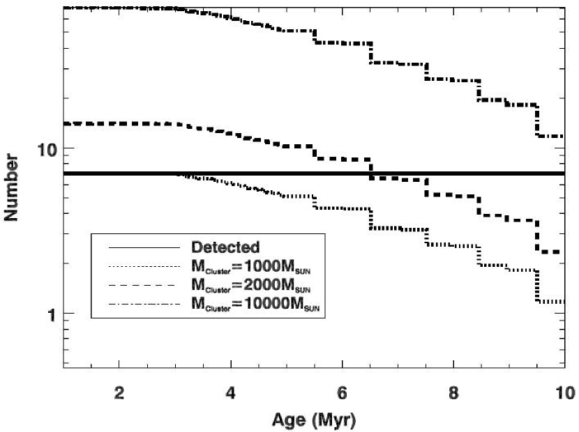
Figure 6: The number of stars with masses over 15 M_⊙ versus the age in a cluster of mass 10³, 2$\times$10³ and 10⁴ M_⊙, respectively. The ‘Salpeter’ IMF is assumed for the mass distribution at the zero age. The Geneva isochrones with solar abundances are used for the evolution of cluster members. The solid straight line indicates the number of massive stars detected in [DBS2003] 45.

To better constrain the age of the cluster, we carry out a Monte-Carlo simulation to estimate the number of massive stars that should be observed within our observing range (M_K$<$18 and 0.4$<$H-Ks$<$0.8) for a cluster. We create a stellar cluster which has an IMF following the ‘Salpeter’ law and has a total mass of 10⁶ M_⊙. In order to improve number statistics, we use the large cluster mass in the simulation. Afterwards, we scale the resulting number down according to an assumed cluster mass. The colors of stars in the cluster are computed for ages between 1 Myr and 10 Myr according to the Geneva isochrones (Schaller et al., 1992). The same distance and average reddening as that derived for [DBS2003] 45 are assumed for the model cluster. Finally, we count the number of stars with masses larger than 15 M_⊙, which is approximately the initial mass of a B0.5 star (Blum et al., 2000). The results are shown in Figure 6. The curves are for a cluster of mass 10⁴ M_⊙, 2.0$\times$10³ M_⊙, and 10³ M_⊙. The simulation predicts that a cluster with M${}_{Cluster}\sim$10³M_⊙ will have only 2-3 massive stars present in our observing range when the cluster is older than 8 Myr. This value is about two times smaller than our detection of 7-8 massive stars. This suggests that either the cluster mass is over 2000 M_⊙ or the cluster age is below 8 Myr. Using a 9.0 Myr isochrone, we estimate that the mass of the cluster is around 1400 M_⊙. An alternative 6.0 Myr isochrone would suggest a cluster mass of 1170 M_⊙. Therefore, the choice of the isochrone does not cause a significant change in the resulting cluster mass to be above 2000 M_⊙. We take this as the evidence to support a younger age for the cluster.

From stellar evolution models, we know that all stars with a mass M$<$120 M_⊙ of a 3 Myr old cluster should be still on the main sequence. Therefore, there should be a limited number of giants or supergiants in the cluster. For stars with an intermediate-mass (M$\sim$25 M_⊙) to evolve off the main sequence, the cluster should be at least 5 Myr old. Our detection of a few evolved stars suggests that [DBS2003] 45 is older than 5 Myr. Therefore stellar models support that [DBS2003] 45 is between 5 and 8 Myr old. This analysis also suggests that the cool supergiant is not a member of the cluster.

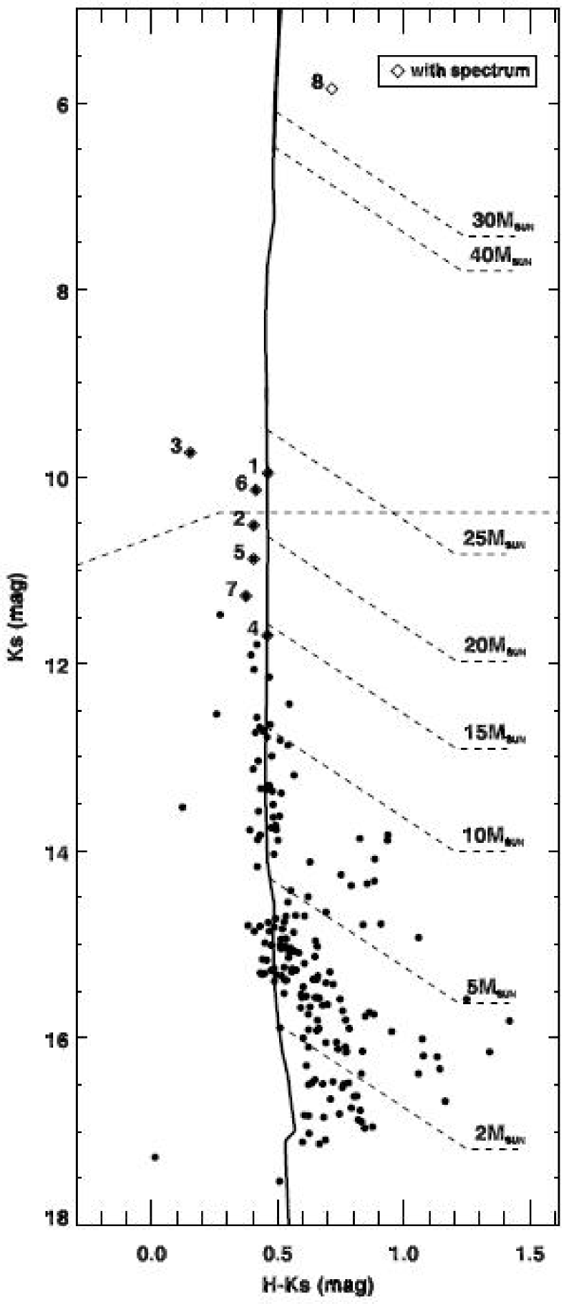
Figure 7: The CMD of [DBS2003] 45 with field contamination removed. The solid line shows the 6 Myr isochrone. The stars with low resolution spectra are signified with diamonds and numbers. The locations of stars of certain initial masses are also indicated with the reddening vector.

In Figure 7, we plot a 6.0 Myr isochrone on the top of the CMD of the observed cluster. As in Figure 5 and 4, the stars with available spectra are indicated with diamonds and numbers. Open squares on the top of some stars indicate that IRAC four color photometric measurements are also available. In the figure, we also indicate the locations of a few stars with different initial masses on the isochrone and the direction of the reddening vector.

4.6 Mass Function

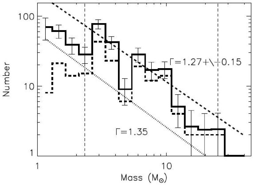
Figure 8: (Left) The mass function of [DBS2003] 45 assuming a 6 Myr isochrone. The dashed histogram shows the result before completeness correction and the solid histogram shows the result after the correction. The fitting result to a power law is indicated for the solid histogram. A classic ‘Salpeter’ model is also plotted. (Right) The slope of the mass function with different bin numbers.

The cluster mass function is based on the stellar magnitudes and the chosen isochrones. The initial mass of a star can be immediately determined if the star is close enough (within 5-$\sigma$ uncertainties) to the isochrone in the CMD. It is simply the corresponding initial mass of the star with the same magnitude on the isochrone. A few stars are on the left side of the isochrone. They could be due to low number statistics. We leave them out in our discussion. The initial masses of stars on the right side of the isochrone are found by extrapolating the reddening vector back toward the isochrone. Figure 8 (left) shows the mass distribution for the final 164 stars with reasonable colors. The Geneva 6 Myr isochrone with solar abundances is used to transform colors to masses. The dashed line histogram shows the distribution before the incompleteness correction and the solid line shows the result after the correction. A set of mass bins equally spaced at the logarithmic scale are chosen to make the histogram. A theoretical (Salpeter) mass function of $\frac{N}{N_{0}}=(\frac{M}{M_{0}})^{-\Gamma}$ with $N(20M_{\odot})=1$ and $\Gamma$=1.35 is also indicated with a straight line in the figure. A regression procedure is used to fit the power law. The regression only uses the bins with at least 3 counts and with a mass bigger than the 50% completeness limit. A slope of $\Gamma$=1.27$\pm$0.15, which is close to the Salpeter value, is found. We notice that the change of isochrone does not produce significant difference in the slope. We estimate the total mass of the cluster by taking the summation of the mass function between the mass range from 0.5 M_⊙ to 45.0 M_⊙, which results in $\sim$1092 M_⊙, $\sim$1170 M_⊙, and $\sim$1393 M_⊙ for the 3 Myr, 6 Myr, and 9 Myr isochrones, respectively.

Our field contamination removed CMD of [DBS2003] 45 has only $<$200 stars. The small size of the sample can result in large statistical uncertainty, especially at the high mass end. There are only a limited number of stars in the bins with the largest central masses. We investigate the effect of the bin number on the resulting slope. By choose different bin numbers, we divide the entire logarithmic mass range into bins of equal sizes. We then populate the bins and fit the resulting mass function to a power law. Figure 8 (right) shows the result of this analysis. The horizontal axis is the number of mass bins that are used. We notice that there is no substantial change in the slope due to the change of the bin size and the slope tends to stabilize at $\sim$-1.25 when the bin number approaches 16 from both ends. Based on this analysis, we conclude that the slope of the mass function is not very different from the Salpeter value.

Compared to Arches cluster at the Galactic center, [DBS2003] 45 has much lower mass. Therefore, our findings can not be used as the evidence to support the statement that the mass function of massive clusters is same as less massive clusters or field stars. Nevertheless, the current data implies that intermediate or low mass clusters may have a similar mass function as field stars. And, the evolutionary effect such as evaporating low mass cluster members to the field during the cluster lifetime seems not change the cluster initial mass function significantly. Our result also does not contradict with Morris (1993), who suggests that clusters near the Galactic center may have shallower IMFs, since [DBS2003] 45 is at a similar distance from the Galactic center as the sun.

However, our finding is based on only one cluster. Low number statistics can be important in this case. Observations and analysis of a large sample of clusters are needed to answer questions such as whether or not the slope of the initial mass function is a function of the cluster mass, the dynamical time and the environment.

4.7 Mid IR Excess

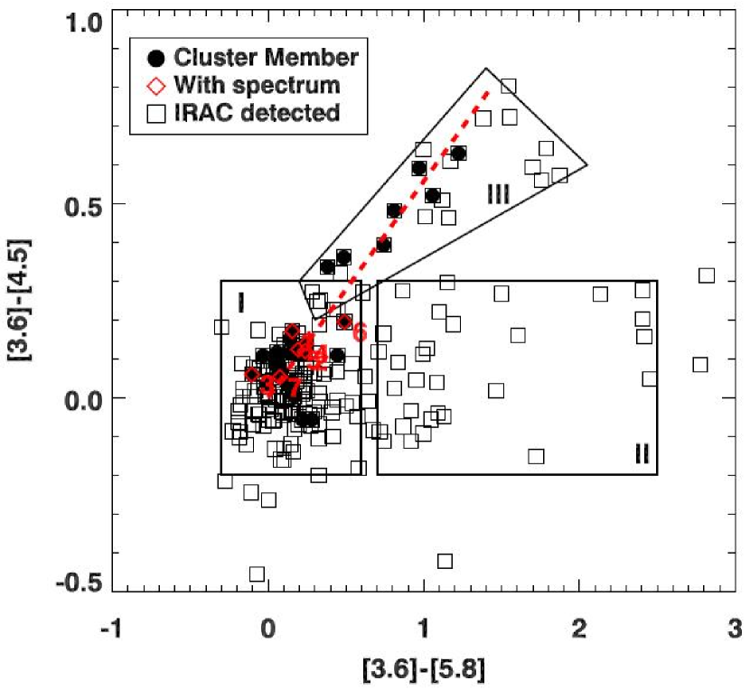
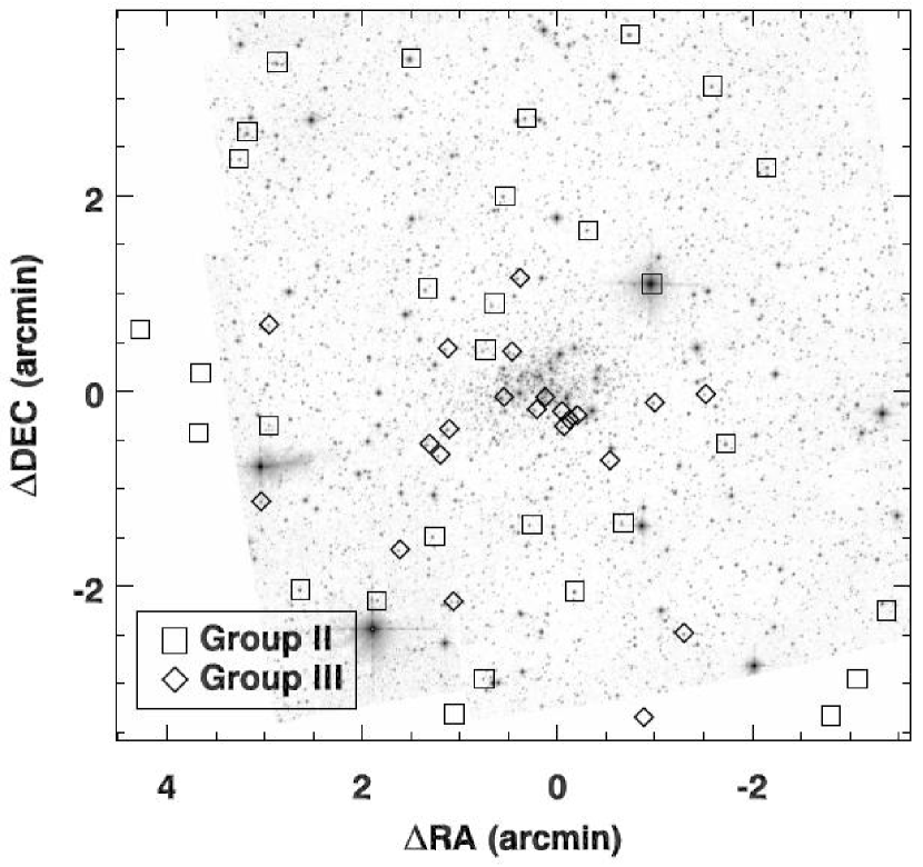
Figure 9: Left: The IRAC color-color diagrams of the cluster. Squares represent data points in the IRAC photometry and filled circles represent the stars with SofI measurements. Stars with spectra are indicated with diamonds and numbers. Right: The locations of stars showing 5.8 $\mu$m excess (Group II) and strong foreground dust extinction (Group III) are indicated with squares and diamonds, respectively. The image is centered at (RA, DEC) = (10^h19^m10.5^s, -58^∘02^′22.6^′′).

As we mentioned earlier, a certain degree of asymmetry in spatial distribution is observed for cluster members. This could suggest patchy extinction toward the field. To confirm this, we plot the photometry of stars obtained by Spitzer/IRAC in Figure 9. We can divide stars on the IRAC M_3.6-4.5 versus M_3.6-5.8 color-color image into three groups, which are indicated by solid-lined boxes. Majority of stars in the lower-left box have M_3.6-4.5$\sim$0.0 and M_3.6-5.8$\sim$0.0 (group I). In the second box, stars have almost constant M_3.6-4.5 but varying M_3.6-5.8 (group II). In the third box, M_3.6-4.5 seems to vary linearly with M_3.6-5.8 and with $\frac{M_{3.6-4.5}}{M_{3.6-4.5}}{\sim}$0.3 (group III).

Stars in group I include almost all stars on the cluster sequence, particularly those close to the assumed isochrone. It is consistent with their small color differences. In the figure, we plot the reddening vector with A_Ks=6.0 mags assuming the intrinsic M_3.6-4.5,0=M_3.6-5.8,0=0.0 and a standard extinction law (A${}_{\lambda}{\varpropto}{\lambda}^{-1.53}$). With A${}_{Ks}{\sim}$0.112A${}_{V}{\sim}$0.8 mag, the values of M_3.6-4.5 and M_3.6-5.8 would be small and within the box we plotted. Group II represents stars with 5.8 $\mu$m excess. The 5.8 $\mu$m and 8.0 $\mu$m channels of IRAC were designed to observe emission from Polycyclic Aromatic Hydrocarbon (PAH) particles in warm interstellar medium. The detection of 5.8 $\mu$m excess may suggest a group of stars with strong PAH emission from their circumstellar envelopes. One interesting fact about these stars is that none of them is present in our cluster CMD. We plot their locations on the top of our Ks band image of the field to check the integrity of our results (right panel of Figure 9), which suggests that those 5.8 $\mu$m bright stars (squares) are all at large distances from the cluster center, including some areas which are not covered by our NIR observations. Thus, it is not a surprise that they are excluded from the cluster population. These stars could be red giant stars in the field, which have lower than main sequence stellar effective temperatures. Stars in group III distribute approximately along the reddening vector and seems to suggest that their colors are strongly affected by varying foreground extinction. Their locations in the Ks band map indicate they do distribute unevenly in the cluster, supporting a patchy extinction interpretation.

Stars left unexplained are those faint in the Ks band and heavily reddened in Figure 7. None of them have an IRAC correspondent. They are probably too faint for IRAC to pick up since the detection limit of IRAC photometry is Ks$\simeq$15.3 mags based on our cross-correlation result between the IRAC catalog and the SofI catalog. Their uneven spatial distribution in the cluster demonstrated by Figure 4 is similar to that of stars in group III in the Figure 9. Therefore, the extra red colors of these faint stars may also be caused by foreground extinction, although we could not rule out the possibility that they have intrinsic colors similar to those in group II. Deeper photometry is needed to clarify on this.

5 Discussion

5.1 The Cluster’s Ionized Bubble

Ionized gas has been observed around massive clusters. In some cases, well-defined bubbles of ionized material and warm dust are seen in radio and infrared wavelengths (Deharveng et al., 2005). It is suggested that dusty material around clusters is heated by energetic photons from cluster members to high temperatures and emits at infrared wavelengths. By examining the properties of radio/IR continuum from the heated material, one can check the consistency between the total energetics and the assumption about the cluster members.

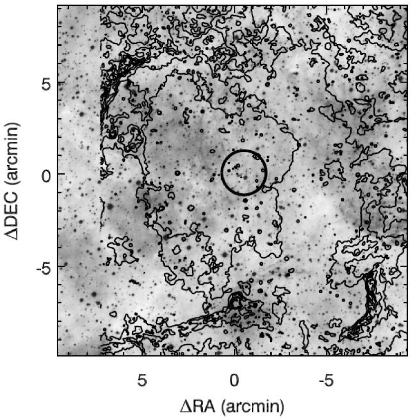
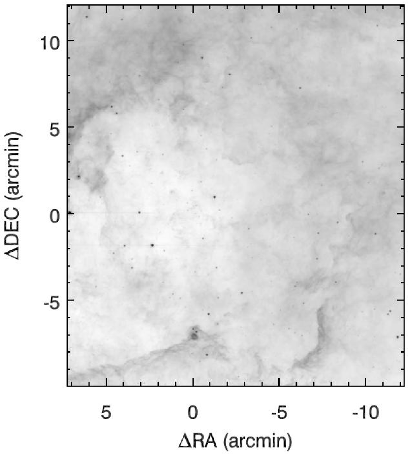
Figure 10: Left: The contours of the IRAC 8.0 $\mu$m image are plotted over the SUPERCOSMOS H_α grey scale image. It is evident that emission from neutral material is mainly come from a ring-like structure around the concentration of emission of ionized gas identified by H_α line emission. The location of the cluster is indicated with a circle. Right: The IRAC 8.0 $\mu$m image is shown in grey scale. Point sources can be seen at several locations along the rim of emission. Both images are centered at (RA, DEC) = (10^h19^m10.5^s, -58^∘02^′22.6^′′).

We over-plot Spitzer IRAC 8.0 $\mu$m emission contours on the top of superCOSMOS H_α emission grey scale image (Figure 10, left). A well-defined cavity of 8.0 $\mu$m emission can be seen around relatively concentrated H_α emission. The location of the identified cluster inside the bubble suggests that the cluster is the source of the ionizing photons. Radio VLA 4850 MHz continuum observations showed that the total continuum flux density of the HII region is 4519$\pm$99 mJy (Wright et al., 1994). In a thermal situation, radio continuum flux luminosity (L${}_{\nu}^{ff}$) and flux density (F${}_{\nu}^{ff}$) are related to the total Lyman continuum photon flux, Q_Ly (Rybicki & Lightman, 1986):

$$L_{\nu}^{ff} = 4{\pi}D^{2}F_{\nu}^{ff}=6.8{\times}10^{-38}T^{0.5}e^{-h{\nu}/kT}\bar{g}_{ff}{\int}N_{e}N_{i}dV$$ (7)

$$Q_{Ly} = {\alpha}_{B}{\int}N_{e}N_{i}dV.$$ (8)

Here D is the heliocentric distance to the HII region, T$\simeq$10⁴K electron temperature, $\bar{g}_{ff}$=5.1 the Gaunt factor, N_e and $N_{i}$ the electron density and the proton density, and ${\alpha}_{B}$ the recombination coefficient. The integral is over the entire volume of the ionized region. We can derive the ionizing photon luminosity to be Q${}_{Ly}{\simeq}$8.2$\times$10⁴⁸ sec^-1. This luminosity corresponds to the total ionizing luminosity of one O8.5 giant star or four B0 type giants (Schaerer & de Koter, 1997; Sternberg et al., 2003). This is consistent with our detection of $\sim$6 early B giants plus one O9 giant. The total energy budget is also consistent with the value from far-IR observations. Deharveng et al. (2005) reported that the far-IR fluxes of IRAS point source associated with the dust ring indicates that the total energy required to power the IRAS source is equivalent to the total luminosity of 10 B1.5V stars. Nevertheless, this energy budget should be the lower limit because it is possible that some fraction of the ionizing photons would escape from the envelope of the surrounding neutral material. From our analysis, it is plausible that the HII region and the bright dust rim around [DBS2003] 45 are excited by the central cluster.

5.2 Triggered Star Formation

Observations indicate that the spatially separated subgroups in given OB associations show systematic differences in stellar age (Blaauw, 1964). Elmegreen & Lada (1977) suggest that the formation of these subgroups is triggered sequentially by the expansion of HII regions. Other scenarios of triggered star formation on different scales have also been proposed (Elmegreen, 1998, and references therein). As we know, in spontaneous star formation the fragmentation and collapse of molecular clouds is due to the loss of internal hydrostatic equilibrium between gravity and supporting forces. On the other hand, external dynamical processes dominate the compression of molecular clouds and initiate the following fragmentation and collapse in triggered star formation scenarios. Triggered star formation is believed to be ubiquitous across star forming regions and galactic disks (Elmegreen, 1998).

Among the proposed scenarios, the “collect and collapse” process at the peripheries of HII regions is particularly interesting because it is thought to be a mechanism by which very massive stars can form (Whitworth et al., 1994, , hereafter W94). In this scenario, star formation is triggered by the propagation of an ionization-shock front into molecular clouds. As the shock front drives into the clouds, neutral material is accumulated and compressed in a layer behind the front. Eventually, this layer of gas becomes gravitationally unstable, fragments, and collapses to form stars. Relatively higher temperature of the shocked gas causes the collapse to start at a higher Jean’s mass.

Despite its appealing to the theory of massive star formation, the collect and collapse process is not convincingly confirmed due to the lack of evidence. This is partially because young stellar objects in the peripheries of HII regions are usually embedded in molecular material and can not be easily detected at optical wavelengths. It is also difficult to distinguish it from other triggering mechanisms since they all introduce systematic differences of the physical properties, e.g. stellar age and mass, between the formed subgroups. With appropriate initial conditions, even spontaneous star formation can cause similar observational features. The initial hierarchical structure in large star forming regions can result in a systematic progression in size, age, and velocity dispersion for OB subgroups formed through the spontaneous process (Elmegreen, 1998). Particularly, the collect and collapse process and the external pressure induced collapse of pre-existing clumps occur on the same scale and cause radial progressions in physical properties, therefore are difficult to be distinguished from each other.

Elmegreen (1998) points out that the collect and collapse process differs from the clump-squeezing process in two aspects. In the former scenario, star formation activities are more like a burst along the ridge of the accumulated gas. In contrast, star formation is continuous throughout the disturbed cloud in the latter case. The collect and collapse scenario tends to form stellar clusters and no star at an intermediate age should exist between the clusters, while the clump compression mechanism tends to form individual stars or small stellar systems and the age distribution of stars is smooth. Therefore, it is possible to distinguish two processes using these properties. We should note that different mechanisms of star formation may be present at the same time. The shock front of an HII region can compress pre-existing globules inside molecular clouds and force them to collapse. At the same time, ambient medium between the globules is swept-up into a layer which can form stars through the collect and collapse process. Nevertheless, observations of young stars along the ridges of HII regions provide supporting evidence of star formation through the collect and collapse mechanism since stars formed through other mechanisms will not distribute preferentially along the shock front.

In a search for infrared sources at HII region peripheries, Deharveng et al. (2005) observed bright and red objects in the dust rim surrounding the ionized gas around [DBS2003] 45. These authors suggest that the point sources are the results of the collect and collapse star formation. Our new observations of [DBS2003] 45 with Spitzer IRAC show a ring-like structure in all four wavelength channels surrounding the cluster. Many bright sources can be seen along the ridge of the structure (Figure 10, right). The light in these mid-IR channels is generally attributed to large molecules such as polycyclic aromatic hydrocarbons (PAHs) (Leger & Puget, 1984). The observed morphology clearly indicates that the ring-like structure is the boundary of the ionized gas and very likely consists of neutral material accumulated during the expansion of the ionization front. Bright and red stellar objects spotted along this structure are the best example of triggered star formation in the swept-up layer around HII regions. Therefore, our observations support that the collect and collapse star formation process is undergoing in [DBS2003] 45. Further support for this star formation mechanism in action would come from observations of the age and mass distributions of the stars along the HII region peripheries. These stars should be significantly younger than the stars belonging to or near the cluster. Observations of similar masses and separations for the newly formed stars along the peripheries would support that they are formed together through the fragmentation of the compressed layer since this process occurs on a typical length scale and produces molecular cores with a typical mass (Whitworth et al., 1994; Elmegreen, 1998).

5.3 Comparison With A Theoretical Model

Whitworth et al. (1994) studied the fragmentation of the dense layer of accumulated material surrounding an expanding HII region and derived formula for the time at which the fragmentation starts (t_frag), the radius of the HII region at that time (R_frag), the column density of the layer, the masses of the fragments (M_frag) and the separation between them. Particularly, W94 showed that both t_frag and R_frag depend weakly on the isothermal sound speed (a_S) in the compressed layer, the number of Lyman continuum photons emitted by the exciting star per second (Q_Ly) and the density of the ambient medium (n₀):

$$R_{frag} {\simeq} 5.8~{}a_{.2}^{4/11}~{}Q_{49}^{1/11}~{}n_{3}^{-6/11}~{}pc$$ (9)

$$t_{frag} {\simeq} 1.56~{}a_{.2}^{7/11}~{}Q_{49}^{-1/11}~{}n_{3}^{-5/11}~{}Myr,$$ (10)

where a_.2=[a_S/0.2 km s^-1], Q₄₉=[Q_Ly/10⁴⁹ s^-1] and n₃=[n₀/10³ cm^-2] are dimensionless variables. They also predicted that the mass of fragments depends strongly on the sound speed a_S:

$$M_{frag} {\simeq} 23~{}a_{.2}^{40/11}~{}Q_{49}^{-1/11}~{}n_{3}^{-5/11}~{}M_{\odot}.$$ (11)

This model has been tested by Dale et al. (2007) using an 1-D smooth particle hydrodynamical code. Although M_frag predicted by Dale et al. is $\sim$2.5 times smaller than the value predicted by the W94 model, the predicted t_frag and R_frag from two models agree with each other within 20 to 25 per cent, suggesting that the W94 model is valid and accurate.

Zavagno et al. (2006)(hereafter Z06) applied the analytical model to a real HII region RCW 79 to estimate its age and other properties. Located at 4.2 kpc (Russeil, 2003), RCW 79 appears to be a circular HII region surrounded by a partially open dust ring. Point sources are observed along the dust ring. This morphology of RCW 79 suggest that the expansion of the HII region triggered the star formation in the dust ring as described by the collect and collapse process (Deharveng et al., 2005). Z06 compared the 1.2 mm continuum, NIR and mid-IR data of RCW 79 with the analytical model and estimated that the dynamical age of RCW 79 is 1.7 Myr. They also estimated that the triggered star formation along the dust ring occurred $\sim$10⁵ years ago. These timescales and the corresponding density ($\sim$2000 cm^-3) of the surrounding molecular material are used to constrain the age of an associated compact HII region and the masses of fragments observed in the ring. The good agreement between the observations and the model predictions indicates that the collect and collapse process is in deed the main triggering mechanism of star formation in the dust ring around RCW 79.

We have not performed molecular line observations to help us constrain the masses of fragments and the sound speed inside the molecular layer in [DBS2003] 45. However, using the morphology of [DBS2003] 45 and the theoretical predictions of W94 (similar to the study of RCW79 by Z06), we can compare the fragmentation age of the expanding bubble with both the bubble’s dynamical age and the age derived for the cluster. The Spitzer IRAC images of [DBS2003] 45 show that the average radius of the ring-like structure is about 8 arcmin. This corresponds to a fragmentation radius of $\leq$10.5 pc at a distance of 4.5 kpc. Adopting an intermediate value (0.4 km s^-1) for a_S, we can derive n${}_{0}\simeq$500 cm^-3 and t${}_{frag}\simeq$3.3 Myr, based on Eq. 9 and 10. Since we assume that the molecular cloud is uniform with a small sound speed and the expansion of the HII region is continuous, the derived n₀ should be considered as the lower limit. Here we have applied Q_Ly=8.2$\times$10⁴⁸ photons per second. Additionally, according to W94 and Dyson & Williams (1997), the radius of the swept-up shell around an evolved HII region grows with time $t$:

$$R{\simeq}4.5~{}Q_{49}^{1/7}~{}n_{3}^{-2/7}~{}t_{M}^{4/7}~{}pc,$$ (12)

where t_M=[t/Myr]. Adopting R=10.5 pc, Q₄₉=0.82 and n₃=0.5, we have $t\simeq$3.3 Myr. The above age estimates are consistent with each other and suggest that the point sources along the dust ridge formed not long time ago. A typical sound speed in the compressed layer is around 0.2-0.6 km s^-1. We used a_S=0.4 km s^-1 in the above calculation, which implies an uncertainty of $\pm$1 Myr for the derived fragmentation age. We have also assumed other values, e.g. the density of the compressed layer, the ionizing luminosity of the central cluster and the size of the ionized bubble, which may introduce additional uncertainty into the derived dynamical age and the fragmentation time of the bubble. If we take the uncertainty into account, 3.3 Myr is in a good agreement with the age of the central cluster of 5 Myr that we have derived in the earlier section.

The above derived numbers rely on the following assumptions: the ionizing photon luminosity of the exciting source is constant during the lifetime of the HII region; the HII region expands within an originally uniform and smooth molecular cloud; the compressed layer by the ionization/shock front has a typical sound speed in dense molecular clouds; the effects of stellar winds and other more complex physical processes are not considered. These assumptions may be oversimplified compared to real star forming regions. More rigorous calculation of the nebular dynamics is well beyond the scope of the current work. Nevertheless, our simple calculations suggest that the radio emission from the HII region is consistent with being powered by the ionizing flux from the cluster. The dynamical age and the fragmentation age of the expanding bubble are consistent with the age we derived for the central cluster. These findings together point to a scenario in which the central cluster has driven the expansion of the HII region into the surrounding medium, and a second generation of star-formation is currently being triggered through the collect and collapse mechanism at the periphery of the bubble.

6 Summary

We present a photometric and spectroscopic study of a stellar cluster candidate on the southern sky. Our study confirms that [DBS2003] 45 is a cluster of a total mass $\sim$10³ M_⊙. The field decontaminated CMD clearly shows a cluster sequence at H-Ks$\simeq$0.45, suggesting an average extinction Av$\sim$7.1 Mags. Based on low-resolution spectroscopy, we identify a few bright cluster members to be early type blue giants/supergiants. The presence of these late O / early B type stars and the absence of any early O type stars and M-type supergiants, suggests an age between 5 and 8 Myr for the identified cluster. A mass function with an approximately Salpeter slope is found for the cluster. The associations of the cluster with the SuperCOSMOS H_α emission morphology and the ring-shaped 8.0$\mu$m structure observed by the infrared camera IRAC on the Spitzer telescope support that the cluster is relatively young and the ambient medium has not been completely dispersed by stellar winds and supernova explosions. Evidence of patchy extinction toward the cluster is found and is consistent with the presence of a population of heavily reddened stars. The presence of infrared point sources along the rim of the dusty bubble supports the mechanism of triggered star formation. Simple calculations of the radio emission and the ages of the HII region support that the identified cluster is the source to drive the expansion of the HII region into the ambient medium and to trigger the formation of new stars.

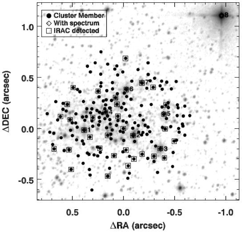
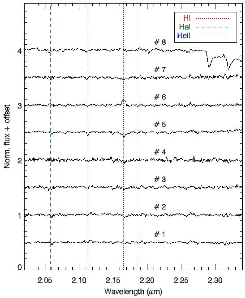
Figure 4: Low-resolution spectra of a few picked stars. The image shows a blowup of the Ks band mosaic of the cluster with symbols indicating different groups of stars in the NIR CMD (Figure 7) and the mid-IR color-color diagram (Figure 9) of the cluster. Filled circles represent stars detected by SofI and stay in the CMD after contamination subtraction. Squares represent stars detected by IRAC. Diamonds and numbers indicate locations of stars with a spectrum shown in the right panel. The image is centered at (RA, DEC) = (10^h19^m10.5^s, -58^∘02^′22.6^′′).

Table 1: Magnitude Calibration Coefficients

Band	a(A)	b(B)	c(C)
h	2.396	1.008	0.007
ks	2.876	0.001	1.019
H	-2.359	0.992	-0.007
Ks	-2.822	-0.001	0.982

Note. — Magnitude transformation coefficients derived through the regression between 2MASS magnitudes and instrumental magnitudes.

Table 2: LIST OF STARS

Star#	RA(J2000)	DEC(J2000)
1	154   48  00.5	- 58   02  23.4
2	154   47  31.7	- 58   02  26.6
3	154   47  15.6	- 58   02  34.6
4	154   47  47.8	- 58   02  13.0
5	154   47  13.8	- 58   02  13.9
6	154   47  35.7	- 58   01  59.5
7	154   47  26.5	- 58   01  55.5
8	154   46  39.9	- 58   01  16.0

Note. — Coordinates of the stars indicated in Figure 4.

References

- Bica et al. (2003) Bica, E., Dutra, C. M., Soares, J., & Barbuy, B. 2003, A&A, 404, 223
- Blaauw (1964) Blaauw, A. 1964, ARA&A, 2, 213
- Blum et al. (2000) Blum, R. D., Conti, P. S., & Damineli, A. 2000, AJ, 119, 1860
- Dale et al. (2007) Dale, J. E., Bonnell, I. A., & Whitworth, A. P. 2007, MNRAS, 375, 1291
- Deharveng et al. (2005) Deharveng, L., Zavagno, A., & Caplan, J. 2005, A&A, 433, 565
- Dias et al. (2002) Dias, W. S., Alessi, B. S., Moitinho, A., & Lépine, J. R. D. 2002, A&A, 389, 871
- Dutra et al. (2003a) Dutra, C. M., Bica, E., Soares, J., & Barbuy, B. 2003a, A&A, 400, 533
- Dutra et al. (2003b) Dutra, C. M., Ortolani, S., Bica, E., Barbuy, B., Zoccali, M., & Momany, Y. 2003b, A&A, 408, 127
- Dyson & Williams (1997) Dyson, J. E. & Williams, D. A. 1997, The physics of the interstellar medium, ed. J. E. Dyson & D. A. Williams
- Elmegreen (1998) Elmegreen, B. G. 1998, in Astronomical Society of the Pacific Conference Series, Vol. 148, Origins, ed. C. E. Woodward, J. M. Shull, & H. A. Thronson, Jr., 150–+
- Elmegreen & Lada (1977) Elmegreen, B. G. & Lada, C. J. 1977, ApJ, 214, 725
- Figer et al. (1999) Figer, D. F., Kim, S. S., Morris, M., Serabyn, E., Rich, R. M., & McLean, I. S. 1999, ApJ, 525, 750
- Froebrich et al. (2007) Froebrich, D., Scholz, A., & Raftery, C. L. 2007, MNRAS, 374, 399
- Hanson et al. (2005) Hanson, M. M., Kudritzki, R.-P., Kenworthy, M. A., Puls, J., & Tokunaga, A. T. 2005, ApJS, 161, 154
- Kim et al. (2006) Kim, S. S., Figer, D. F., Kudritzki, R. P., & Najarro, F. 2006, ApJ, 653, L113
- Kroupa (2001) Kroupa, P. 2001, MNRAS, 322, 231
- Kroupa (2002) —. 2002, Science, 295, 82
- Leger & Puget (1984) Leger, A. & Puget, J. L. 1984, A&A, 137, L5
- Lejeune & Schaerer (2001) Lejeune, T. & Schaerer, D. 2001, A&A, 366, 538
- Moorwood et al. (1998) Moorwood, A., Cuby, J.-G., & Lidman, C. 1998, The Messenger, 91, 9
- Morris (1993) Morris, M. 1993, ApJ, 408, 496
- Parker et al. (2005) Parker, Q. A., Phillipps, S., Pierce, M. J., Hartley, M., Hambly, N. C., Read, M. A., MacGillivray, H. T., Tritton, S. B., Cass, C. P., Cannon, R. D., Cohen, M., Drew, J. E., Frew, D. J., Hopewell, E., Mader, S., Malin, D. F., Masheder, M. R. W., Morgan, D. H., Morris, R. A. H., Russeil, D., Russell, K. S., & Walker, R. N. F. 2005, MNRAS, 362, 689
- Rieke & Lebofsky (1985) Rieke, G. H. & Lebofsky, M. J. 1985, ApJ, 288, 618
- Russeil (2003) Russeil, D. 2003, A&A, 397, 133
- Rybicki & Lightman (1986) Rybicki, G. B. & Lightman, A. P. 1986, Radiative Processes in Astrophysics (Radiative Processes in Astrophysics, by George B. Rybicki, Alan P. Lightman, pp. 400. ISBN 0-471-82759-2. Wiley-VCH , June 1986.)
- Salpeter (1955) Salpeter, E. E. 1955, ApJ, 121, 161
- Scalo (1998) Scalo, J. 1998, in Astronomical Society of the Pacific Conference Series, Vol. 142, The Stellar Initial Mass Function (38th Herstmonceux Conference), ed. G. Gilmore & D. Howell, 201–+
- Schaerer & de Koter (1997) Schaerer, D. & de Koter, A. 1997, A&A, 322, 598
- Schaller et al. (1992) Schaller, G., Schaerer, D., Meynet, G., & Maeder, A. 1992, A&AS, 96, 269
- Sternberg et al. (2003) Sternberg, A., Hoffmann, T. L., & Pauldrach, A. W. A. 2003, ApJ, 599, 1333
- Stolte et al. (2002) Stolte, A., Grebel, E. K., Brandner, W., & Figer, D. F. 2002, A&A, 394, 459
- Whitworth et al. (1994) Whitworth, A. P., Bhattal, A. S., Chapman, S. J., Disney, M. J., & Turner, J. A. 1994, MNRAS, 268, 291
- Wright et al. (1994) Wright, A. E., Griffith, M. R., Burke, B. F., & Ekers, R. D. 1994, ApJS, 91, 111
- Zavagno et al. (2006) Zavagno, A., Deharveng, L., Comerón, F., Brand, J., Massi, F., Caplan, J., & Russeil, D. 2006, A&A, 446, 171
- Zinnecker & Yorke (2007) Zinnecker, H. & Yorke, H. W. 2007, ARA&A, 45, 481