Abstract

We examine the possible trajectories of a classical particle, trapped in a two-dimensional infinite rectangular well, using the Hamilton-Jacobi equation. We observe that three types of trajectories are possible: periodic orbits, open orbits and some special trajectories when the particle gets pocketed.

1 Introduction

The so-called ‘Billiard systems’, describing the motion of a classical particle (a point ball) moving within a closed boundary of different shapes, and bouncing perfectly from the walls, have attracted the attention of various scientists for a long time [1]. Though the system appears simple, nevertheless it is very rich and instructive, as the dynamics depends particularly on the shape of the enclosure [2, 3]. Consequently, such systems have been studied both classically as well as in the realm of quantum mechanics [4, 5]. It is assumed that motion between collisions with the wall is in a straight line, and at each bounce there is simple reflection with no dissipation, i.e., the ball follows a path just like a light ray with a boundary wall which is a perfect mirror [2]. Enclosures of different shapes have been studied widely in the framework of Hamilton-Jacobi theory and interesting results obtained. For example, circular and elliptic enclosures with rigid boundaries have been considered in [2] and the orbits traced out. In particular, for such circular and elliptic enclosures a second conserved quantity has been found other than the Hamiltonian, leading to integrability and order. The trajectory for a circular enclosure is found to be a succession of chords such that the angular momentum of the particle about the centre remains constant through successive bounce at the boundary. For the elliptical enclosure the second conserved quantity is the product of the angular momentum of the particle measured about the two foci of the ellipse. In [6] the periodic trajectories of a particle trapped in an infinite square well have been explored, using the Hamilton-Jacobi equation in 2-dimensions. Motivated by such efforts, our aim in this work is to study the same for a conventional billiard, modelled by an infinite rectangular well potential.

In section 2, we touch upon the Hamilton-Jacobi (H-J) equation [3,7,8] and discuss the action-angle variables. In Section 3, we apply the H-J equation to investigate the periodic classical trajectories of a particle trapped inside a rectangular billiard with infinite barriers. The different types of orbits, viz., periodic orbits, open trajectories, and those special trajectories when the ball hits one of the corners and gets pocketed, are discussed in detail in Section 4, with suitable illustrations. Finally, Section 5 is kept for Conclusions and remarks.

2 Hamilton-Jacobi Equation

If $(q,p,t)$ is cannonically related to $(Q,P,t)$ under the influence of a Hamiltonian $H(q,p,t)$ where $q=(q_{1},q_{2},...,q_{n})$ and $p=(p_{1},p_{2},...,p_{n})$ are generalized coordinates and canonical momenta respectively, then, as is well known, the Hamilton Jacobi equation is

$$\frac{\partial S}{\partial t}+H\left(q,\frac{\partial S}{\partial q},t\right)=0$$ (1)

where S is the Hamilton’s principal function

Writing ,

$$S=W(q_{1},q_{2},\cdots,q_{n})-\alpha_{1}t$$ (2)

where the time-independent function $W(q)$ is Hamilton’s characteristic function and the constant $\alpha_{1}$ is the energy $E$. This transforms the H-J equation to

$$H\left(q,\frac{\partial S}{\partial q}\right)=E$$ (3)

For integrable systems there is a natural set of co-ordinates and momenta which is particularly convenient and useful [3, 7]. These systems have $n$ distinct constants of motion and we can transform to a new set of coordinates $w_{i}$ and momenta $J_{i}$ in such a way that
$*$ the Hamiltonian form of the equations of motion is preserved : $K(J_{j})\equiv H$,
$*$ the new momenta $J_{i}$ are all constants of motion,
$*$ the new coordinates $w_{i}$ are all ignorable.
Writing the Hamilton’s characteristic function as $W=W(q,J)$, the angle variables $w_{i}$ and the corresponding canonically conjugate action variables $J_{i}$ are given by

$$\dot{w}_{j}~{}=~{}\displaystyle\frac{\partial K(J)}{\partial J_{j}}~{}\equiv~{}\nu(J)$$ (4)

$$\dot{J}_{j}~{}=~{}\displaystyle-\frac{\partial K}{\partial w_{j}}~{}=~{}0$$ (5)

For Hamilton’s equations to be form-invariant it is necessary that the change of variables $(q,p)\rightarrow(w,J)$ should preserve areas, so that a natural choice for $J$ is given by

$$J=\displaystyle\oint pdq$$ (6)

where the integration is carried over a complete period of libration or rotation, as the case may be. The angle variable, which is the generalized coordinate conjugate to $J$, is defined by the transformation equation

$$w(J)=\displaystyle\frac{\partial W}{\partial J}$$ (7)

It is evident from (4) that the angle variables evolve at a uniform rate, given by

$$w_{j}=\nu_{j}t+\beta_{j}$$ (8)

where $\nu_{j}$ is the frequency associated with the periodic motion and $\beta_{j}$ are constants. The use of action-angle variables thus provides a powerful technique for obtaining the frequency of periodic motion without finding a complete solution to the motion of the system.

3 Motion of a particle in a 2-dim. rectangular well

With the above background, let us investigate the nature of the trajectories when the particle is in an infinite rectangular well, with centre at $(0,0)$ and vertices at $(\pm a\ ,\ \pm b)$ :

$$V(x,y)=\left\{\begin{array}[]{lcl}0\qquad\ \ \ \ \ \ \ |x|<a\qquad{\rm{and}}\qquad|y|<b\\ \\ \infty\qquad\ \ \ \ \ \ |x|>a\qquad{\rm{and}}\qquad|y|>b\\ \end{array}\right.$$ (9)

A canonical transformation from $(q,p)\rightarrow(Q,P)$, i.e., to new variables $(\beta,\alpha)$ which are constants in time, and, employing a type-two generating function $F_{2}(q,P,t)\equiv S(q,\alpha,t)$, with the assumption that $H$ does not depend on $t$ explicitly, (3) reduces to the form

$$\frac{1}{2m}\left[\left(\frac{\partial W}{\partial x}\right)^{2}+\left(\frac{\partial W}{\partial y}\right)^{2}\right]=E$$ (10)

Writing $W(q)=X(x)+Y(y)$ in (10), the constants of motion are obtained as

$$\left(\frac{dX}{dx}\right)^{2}=\alpha_{x}^{2}\qquad,\qquad\displaystyle\left(\frac{dY}{dy}\right)^{2}=\alpha_{y}^{2}$$ (11)

with $\displaystyle E=\frac{1}{2m}\left(\alpha_{x}^{2}+\alpha_{y}^{2}\right)$, yielding

$$p_{x}=\pm\alpha_{x}\qquad,\qquad p_{y}=\pm\alpha_{y}$$ (12)

the signs showing the reversal in the direction of motion of the particle each time it hits the barriers at $x=\pm a$ and $y=\pm b$.
The action variables can now be calculated easily from (6) and turn out to be

$$J_{x}=4a\alpha_{x}$$ (13)

$$J_{y}=4b\alpha_{y}$$ (14)

so that $E$ becomes

$$E=\displaystyle\frac{1}{32m}\left(\frac{J_{x}^{2}}{a^{2}}+\frac{J_{y}^{2}}{b^{2}}\right)$$ (15)

Thus the natural frequencies of the system are obtained from (4) to be

$$\nu_{x}=\displaystyle\frac{\partial E}{\partial J_{x}}=\frac{J_{x}}{16ma^{2}}\qquad,\qquad\nu_{y}=\displaystyle\frac{\partial E}{\partial J_{y}}=\frac{J_{y}}{16mb^{2}}$$ (16)

which, with the help of (13) and (14) read equivalently

$$\nu_{x}=\displaystyle\frac{p_{x}}{4ma}\qquad,\qquad\nu_{y}=\frac{p_{y}}{4mb}$$ (17)

Thus the natural frequencies are functions of the particle velocity and the dimensions of the well. Consequently, three types of trajectories are possible for the particle trapped in the rectangular well, as discussed below.

4 Possible Trajectories

In this section we shall discuss in detail the three possible trajectories of the trapped particle, viz.,
1. Periodic Trajectories
2. Open Trajectories
3. Special Trajectories when the particle hits one of the corners and gets pocketed.

4.1 Periodic Trajectories :

One of our primary aims in this work is to study periodic or closed trajectories. It is evident from equation (17), for the particle to execute periodic motion, it must return to the starting point with its initial momenta after a certain time. This is possible only if

$$T=n_{x}T_{x}=n_{y}T_{y}$$ (18)

where $T_{x}$ and $T_{y}$ represent the time in which the particle reaches the starting point with its initial momenta in the $x$ and $y$ directions respectively, $T$ is the time period of the orbit, and $n_{x}\ ,\ n_{y}$ are integers. Thus, if the particle starts from the origin at an angle $\theta$ to the $x$ direction, where

$$\tan\ \theta=\frac{p_{y}}{p_{x}}$$ (19)

then, for closed orbits $\tan\ \theta$ must be rational , with the time period given by (18). With the help of (17), eq. (19) may be rearranged to give

$$\tan\ \theta=\displaystyle\frac{b\nu_{y}}{a\nu_{x}}=\frac{bT_{x}}{aT_{y}}=\frac{bn_{y}}{an_{x}}$$ (20)

We shall illustrate this with a couple of explicit examples below, the particle starting from the origin in each case. The corresponding closed orbits are plotted in Figures 1 and 2; the starting trajectory is shown in blue, the intermediate ones in red, and the closing one in black.

4.1.1 Some explicit examples for periodic trajectories

Case 1 : $n_{y}=1,n_{x}=4$ , i.e., $\displaystyle\frac{p_{y}}{p_{x}}=\frac{b}{4a}$

This case is illustrated in Figure 1. The trajectories traced out by the particle are

$$\begin{array}[]{lcl}x&=&\displaystyle\frac{p_{x}}{m}t\qquad\qquad\qquad\qquad\qquad\ y=\displaystyle\frac{p_{y}}{m}t\qquad\qquad\qquad\qquad\qquad\ \ \ t_{16(r-1)}\leq t\leq t_{16r-15}\\ \\ x&=&\displaystyle-\frac{p_{x}}{m}\left(t-t_{16r-15}\right)+a\qquad\ \ \ y=\displaystyle\frac{p_{y}}{m}\left(t-t_{16r-15}\right)+\frac{b}{4}\qquad\ \ \ \ \ t_{16r-15}\leq t\leq t_{16r-14}\\ \\ x&=&\displaystyle-\frac{p_{x}}{m}\left(t-t_{16r-14}\right)\qquad\qquad\ \ y=\displaystyle\frac{p_{y}}{m}\left(t-t_{16r-14}\right)+\frac{b}{2}\qquad\ \ \ \ \ t_{16r-14}\leq t\leq t_{16r-13}\\ \\ x&=&\displaystyle\frac{p_{x}}{m}\left(t-t_{{16r-13}}\right)-a\qquad\qquad y=\displaystyle\frac{p_{y}}{m}\left(t-t_{16r-13}\right)+\frac{3b}{4}\qquad\ \ \ \ t_{16r-13}\leq t\leq t_{16r-12}\\ \\ x&=&\displaystyle\frac{p_{x}}{m}\left(t-t_{16r-12}\right)\qquad\qquad\ \ \ \ \ y=\displaystyle-\frac{p_{y}}{m}\left(t-t_{16r-12}\right)+b\qquad\ \ \ \ t_{16r-12}\leq t\leq t_{16r-11}\\ \\ x&=&\displaystyle-\frac{p_{x}}{m}\left(t-t_{16r-11}\right)+a\qquad\ \ \ \ y=\displaystyle-\frac{p_{y}}{m}\left(t-t_{16r-11}\right)+\frac{3b}{4}\qquad\ \ t_{16r-11}\leq t\leq t_{16r-10}\\ \\ x&=&\displaystyle-\frac{p_{x}}{m}\left(t-t_{16r-10}\right)\qquad\qquad\ \ \ y=\displaystyle-\frac{p_{y}}{m}\left(t-t_{16r-10}\right)+\frac{b}{2}\qquad\ \ \ \ t_{16r-10}\leq t\leq t_{16r-9}\\ \\ x&=&\displaystyle\frac{p_{x}}{m}\left(t-t_{16r-9}\right)-a\qquad\qquad\ \ y=\displaystyle-\frac{p_{y}}{m}\left(t-t_{16r-9}\right)+\frac{b}{4}\qquad\ \ \ \ t_{16r-9}\leq t\leq t_{16r-8}\\ \\ x&=&\displaystyle\frac{p_{x}}{m}(t-t_{16r-8})\qquad\qquad\qquad\ \ y=\displaystyle-\frac{p_{y}}{m}(t-t_{16r-8})\qquad\qquad\ \ \ t_{16r-8}\leq t\leq t_{16r-7}\\ \\ x&=&\displaystyle-\frac{p_{x}}{m}\left(t-t_{16r-7}\right)+a\qquad\ \ \ \ y=\displaystyle-\frac{p_{y}}{m}\left(t-t_{16r-7}\right)-\frac{b}{4}\qquad\ \ \ \ t_{16r-7}\leq t\leq t_{16r-6}\\ \\ x&=&\displaystyle-\frac{p_{x}}{m}\left(t-t_{16r-6}\right)\qquad\qquad\ \ \ y=\displaystyle-\frac{p_{y}}{m}\left(t-t_{16r-6}\right)-\frac{b}{2}\qquad\ \ \ \ \ t_{16r-6}\leq t\leq t_{16r-5}\\ \\ x&=&\displaystyle\frac{p_{x}}{m}\left(t-t_{{16r-5}}\right)-a\qquad\qquad\ y=\displaystyle-\frac{p_{y}}{m}\left(t-t_{16r-5}\right)-\frac{3b}{4}\qquad\ \ \ \ t_{16r-5}\leq t\leq t_{16r-4}\\ \\ x&=&\displaystyle\frac{p_{x}}{m}\left(t-t_{16r-4}\right)\qquad\qquad\ \ \ \ \ \ y=\displaystyle\frac{p_{y}}{m}\left(t-t_{16r-4}\right)-b\qquad\ \ \ \ t_{16r-4}\leq t\leq t_{16r-3}\\ \\ x&=&\displaystyle-\frac{p_{x}}{m}\left(t-t_{16r-3}\right)-a\qquad\ \ \ \ \ y=\displaystyle\frac{p_{y}}{m}\left(t-t_{16r-3}\right)-\frac{b}{4}\qquad\ \ t_{16r-3}\leq t\leq t_{16r-2}\\ \\ x&=&\displaystyle-\frac{p_{x}}{m}\left(t-t_{16r-2}\right)\qquad\qquad\ \ \ \ y=\displaystyle\frac{p_{y}}{m}\left(t-t_{16r-2}\right)-\frac{b}{2}\qquad\ \ \ \ t_{16r-2}\leq t\leq t_{16r-1}\\ \\ x&=&\displaystyle\frac{p_{x}}{m}\left(t-t_{16r-1}\right)-a\qquad\qquad\ \ y=\displaystyle\frac{p_{y}}{m}\left(t-t_{16r-1}\right)-\frac{b}{4}\qquad\ \ \ \ t_{16r-1}\leq t\leq t_{16r}\\ \\ \end{array}$$ (21)

where $r=1,2,\cdots$ and $t_{n}=\displaystyle(2n-1)\frac{ma}{p_{x}}\ ,\ n=1,2,\cdots$
Thus, in this case, the trajectories are periodic when the velocities of the particle in the $x$ and $y$ directions are such that the time taken by the particle to cover distance $a$ in the $x$ direction, is the same as the time it takes to cover the distance $b/4$ in the $y$ direction :

$$t_{1}=\frac{ma}{p_{x}}=\frac{mb}{4p_{y}}$$

This gives the time period as $T=4T_{x}=T_{y}$, where $T_{x}=4t_{1}$ and $T_{y}=16t_{1}$. This is a new result not discussed for $a=b$ in ref. [6].

Case 2 : $n_{y}=2,n_{x}=3$ , i.e., $\displaystyle\frac{p_{y}}{p_{x}}=\frac{2b}{3a}$

This case is illustrated in Figure 2. The particle can be shown to trace out the following trajectories :

$$\begin{array}[]{lcl}x&=&\displaystyle\frac{p_{x}}{m}t\qquad\qquad\qquad\qquad\qquad\ y=\displaystyle\frac{p_{y}}{m}t\qquad\qquad\qquad\qquad\qquad\ \ \ t_{12(r-1)}\leq t\leq t_{12r-11}\\ \\ x&=&\displaystyle-\frac{p_{x}}{m}\left(t-t_{12r-11}\right)+a\qquad\ \ \ y=\displaystyle\frac{p_{y}}{m}\left(t-t_{12r-11}\right)+\frac{2b}{3}\qquad\ \ \ t_{12r-11}\leq t\leq t_{12r-10}\\ \\ x&=&\displaystyle-\frac{p_{x}}{m}\left(t-t_{12r-10}\right)+\frac{a}{2}\qquad\ \ \ y=\displaystyle-\frac{p_{y}}{m}\left(t-t_{12r-10}\right)+b\qquad\ \ \ \ \ t_{12r-10}\leq t\leq t_{12r-9}\\ \\ x&=&\displaystyle\frac{p_{x}}{m}\left(t-t_{{12r-9}}\right)-a\qquad\qquad\ y=\displaystyle-\frac{p_{y}}{m}\left(t-t_{12r-9}\right)\qquad\qquad t_{12r-9}\leq t\leq t_{12r-8}\\ \\ x&=&\displaystyle\frac{p_{x}}{m}\left(t-t_{12r-8}\right)+\frac{a}{2}\qquad\qquad\ y=\displaystyle\frac{p_{y}}{m}\left(t-t_{12r-8}\right)-b\qquad\ \ \ \ t_{12r-8}\leq t\leq t_{12r-7}\\ \\ x&=&\displaystyle-\frac{p_{x}}{m}\left(t-t_{12r-7}\right)+a\qquad\ \ \ \ y=\displaystyle\frac{p_{y}}{m}\left(t-t_{12r-7}\right)-\frac{2b}{3}\qquad\ \ t_{12r-7}\leq t\leq t_{12r-6}\\ \\ x&=&\displaystyle-\frac{p_{x}}{m}\left(t-t_{12r-6}\right)\qquad\qquad\ \ \ y=\displaystyle\frac{p_{y}}{m}\left(t-t_{12r-6}\right)\qquad\qquad\ \ \ t_{12r-6}\leq t\leq t_{12r-5}\\ \\ x&=&\displaystyle\frac{p_{x}}{m}\left(t-t_{12r-5}\right)-a\qquad\qquad\ y=\displaystyle\frac{p_{y}}{m}\left(t-t_{12r-5}\right)+\frac{2b}{3}\qquad\ \ \ \ t_{12r-5}\leq t\leq t_{12r-4}\\ \\ x&=&\displaystyle\frac{p_{x}}{m}(t-t_{12r-4})-\frac{a}{2}\qquad\ \ \ \ y=\displaystyle-\frac{p_{y}}{m}(t-t_{12r-4})-b\qquad\qquad\ \ \ t_{12r-4}\leq t\leq t_{12r-3}\\ \\ x&=&\displaystyle-\frac{p_{x}}{m}\left(t-t_{12r-3}\right)+a\qquad\ \ \ \ \ y=\displaystyle-\frac{p_{y}}{m}\left(t-t_{12r-3}\right)\qquad\ \ \ \ t_{12r-3}\leq t\leq t_{12r-2}\\ \\ x&=&\displaystyle-\frac{p_{x}}{m}\left(t-t_{12r-2}\right)-\frac{a}{2}\qquad\ \ \ \ y=\displaystyle\frac{p_{y}}{m}\left(t-t_{12r-2}\right)-b\qquad\ \ \ \ \ t_{12r-2}\leq t\leq t_{12r-1}\\ \\ x&=&\displaystyle\frac{p_{x}}{m}\left(t-t_{{12r-1}}\right)-a\qquad\qquad\ y=\displaystyle\frac{p_{y}}{m}\left(t-t_{12r-1}\right)-\frac{2b}{3}\qquad\ \ \ \ t_{12r-1}\leq t\leq t_{12r}\\ \\ \end{array}$$ (22)

where $r=1,2,\cdots$ and $t_{n}=\displaystyle(2n-1)\frac{ma}{p_{x}}\ ,\ n=1,2,\cdots$

It is easy to observe from Figure 2 that in this case $t_{2}=3t_{1}/2,\ t_{3}=3t_{1},\ t_{4}=9t_{1}/2,\ t_{5}=5t_{1}$, etc. Thus $T_{x}=t_{5}-t_{1}=\displaystyle 4t_{1}$ and $T_{y}=t_{8}-t_{2}=\displaystyle 6t_{1}$, where $t_{1}=\displaystyle\frac{ma}{p_{x}}=\frac{2mb}{3p_{y}}$, giving $T=12t_{1}=3T_{x}=2T_{y}$. Note that we get back the result of [6] for $a=b$.

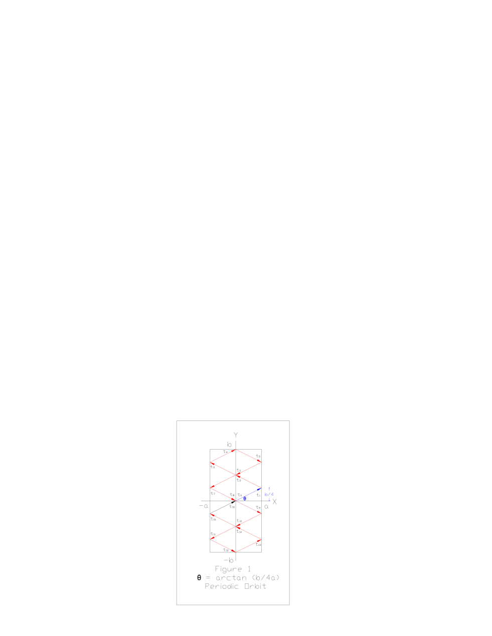
Figure 1: This shows a periodic trajectory for $\displaystyle n_{y}=1,\ n_{x}=4$, so that $\tan\theta=\displaystyle\frac{p_{y}}{p_{x}}=\frac{b}{4a}$

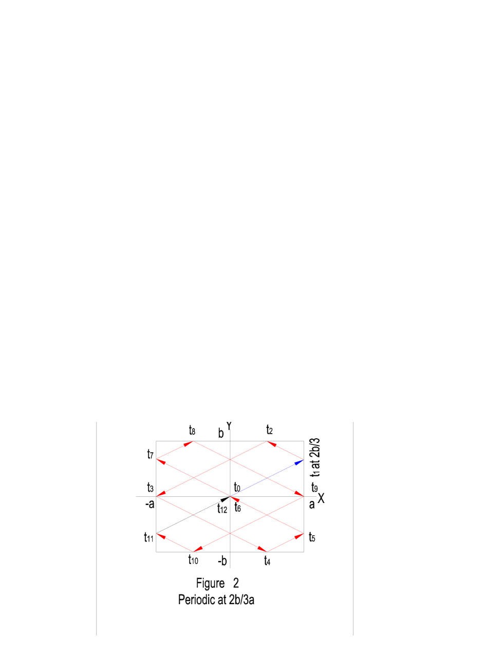
Figure 2: This shows a periodic trajectory for $\displaystyle n_{y}=2,n_{x}=3$ , so that $\tan\theta=\displaystyle\frac{p_{y}}{p_{x}}=\frac{2b}{3a}$

4.2 Open Trajectories :

If the initial angle $\theta$ is such that $\displaystyle\frac{p_{y}}{p_{x}}$ is irrational, then the orbit is an open one. This is due to the fact that the time periods in the $x$ and $y$ directions are such that one cannot find integral values of $n_{x}$ , $n_{y}$ satisfying equation (18). We have traced out such a trajectory in Figure 3, for $\theta=30^{0}$, starting with the blue line. Even after multiple reflections from the perfectly elastic walls of the rectangular well (shown by the red paths) the orbit does not close as is evident from the black line with the arrowhead.

4.3 Special Trajectories when the billiard ball hits a corner:

We now address the interesting case of special non-periodic trajectories when the particle hits one of the corners of the billiard table and gets pocketed. For the ball to hit either the right or left wall, the distance travelled in the $x$ direction is $(4n\pm 1)a$, where $n$ is an integer. Similarly, to hit the top or bottom wall the distance travelled in the $y$ direction is $(4m\pm 1)b$, where $m$ is also an integer. If the ball hits a corner then these two conditions must be satisfied simultaneously. Thus, if the particle hits a corner in time $t$, then

$$\frac{v_{y}t}{v_{x}t}=\displaystyle\frac{\left(4m\pm 1\right)b}{\left(4n\pm 1\right)a}$$ (23)

and the condition for the billiard ball to get pocketed reduces to

$$\frac{p_{y}}{p_{x}}=\displaystyle\frac{\left(4m\pm 1\right)b}{\left(4n\pm 1\right)a}$$ (24)

If the numerator has $+ve$ ($-ve)$) sign in (24), then the ball hits one of the two corners where $y$ is positive (negative). Similarly, if the denominator has $+ve$ ($-ve)$) sign in (24), then the ball hits one of the two corners where $x$ is positive (negative). From equations (19), (20) and (24), it is obvious that this occurs for odd integral values of both $n_{x}$ and $n_{y}$. Based on this we summarize in Table 1 the corner in which the ball will get pocketed. It may be mentioned that we assign the following numbers to the respective corners : $(a,b)$ as corner 1, $(-a,b)$ as corner 2, $(-a,-b)$ as corner 3, and $(a,-b)$ as corner 4. We shall trace out the actual trajectories in Fig 4. It is observed that the predicted corners are in fact the actual ones.

Table 1 :

$\displaystyle n_{y}/n_{x}$	sign (numerator, denominator)	corner
$1/3$	$(-,+)$	2
$1/5$	$(+,+)$	1
$1/7$	$(-,+)$	2
$1/9$	$(+,+)$	1
$3/7$	$(-,-)$	3
$5/7$	$(-,+)$	2
$3/5$	$(+,-)$	4
$5/9$	$(+,+)$	1
$7/9$	$(+,-)$	4

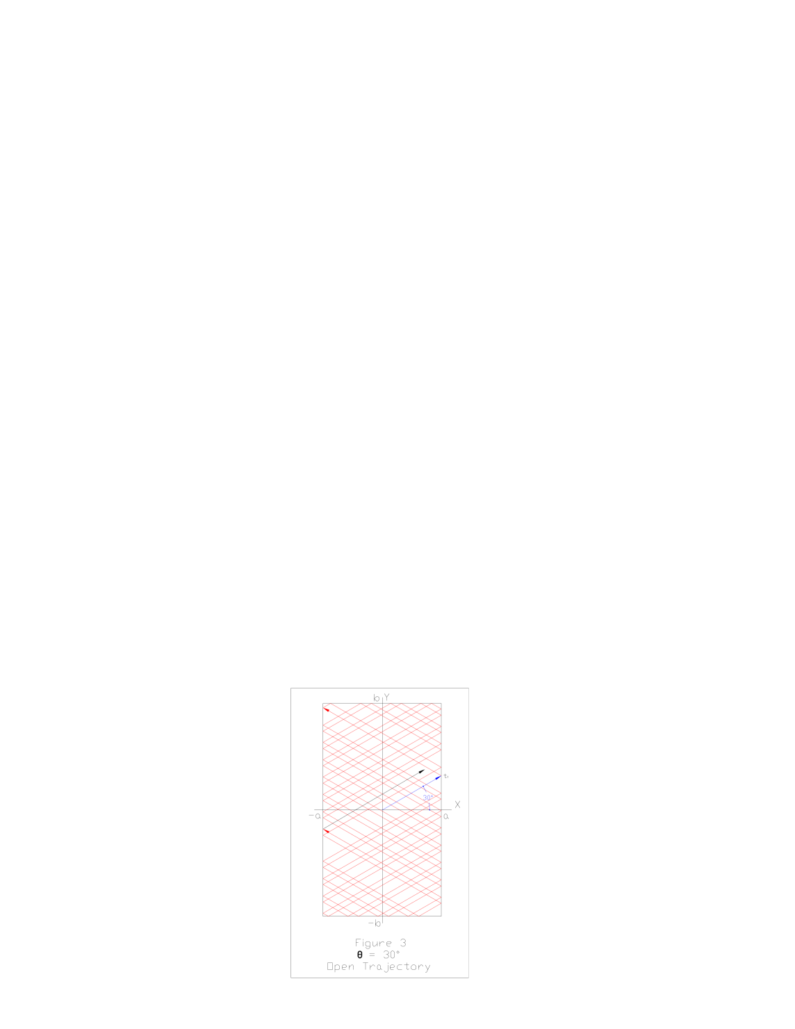
Figure 3: This shows an open trajectory for $\theta=30^{o}$

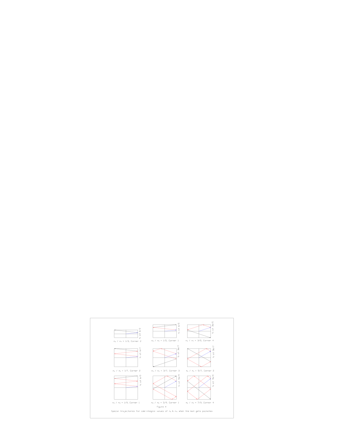
Figure 4: This shows some of the special trajectories for odd integral values of both $n_{y}$ and $n_{x}$ , when the billiard ball hits one of the corners and gets pocketed. The corners predicted in Table 1 agree with those actually traced out in this figure

5 Conclusions

To conclude, we have studied the motion of a classical point particle, trapped in an infinite rectangular well with perfectly elastic boundaries, using the action-angle variables in the Hamilton-Jacobi formalism. In particular, we have determined the natural frequencies of the system in the $x$ and $y$ directions. These frequencies given by $\nu_{x}$, $\nu_{y}$ in eq. (16), are found to be functions of the velocity of the trapped particle, and the dimensions of the rectangular well, viz., $a,\ b$ respectively. It may be worth mentioning here that since the potential $V=0$ inside the enclosure, the magnitudes of the particle momenta in the $x$ and $y$ directions ($p_{x}$ and $p_{y}$) do not change inside the well. We have established a definite relationship between the orbit traced out by the classical particle and the initial angle (say $\theta$ with the $x$ axis) at which the particle starts from rest from the origin, i.e., on the ratio $p_{y}/p_{x}$. When $p_{x}$ , $p_{y}$ are both rational, depending on the values of $n_{x}$ and $n_{y}$, some orbits with definite periodicity have been illustrated in Figures 1 and 2. In these cases one can find integral values of $n_{x}\ ,\ n_{y}$ for which the relationship $n_{x}T_{x}=n_{y}T_{y}$ holds, and the time period of the periodic motion is obtained as $T=n_{x}T_{x}=n_{y}T_{y}$.

On the other hand, if the initial angle $\theta$ is such that $\tan\ \theta=p_{y}/p_{x}$ is irrational, the orbit is an open one. Such an open orbit has been sketched in Figure 3, for the particular value of $\theta=30^{0}$.

Still more interesting are the cases when the billiard ball falls into one of the pockets. We have shown that this occurs for odd integral values of both $n_{x}$ and $n_{y}$. A few such trajectories are plotted in Figure 4. In fact, our conjecture can even predict accurately which corner the particle would hit. The excellent agreement between Table 1 and Fig 4 gives credence to our conjecture.

Additionally, we have observed that the qualitative picture does not depend on the dimensions of the well, i.e. on the ratio $a/b$. For the special case $a=b$, i.e., an infinite square well, our results reduce to those of ref [6].

6 Acknowledgement

One of us (BB) thanks Prof. C.Quesne, PNTPM, University of Libre, Brussels, for clarification of several points concerning the infinite well problem, while another (AS) thanks Mr. Debayan Saha, Indian Institute of Technology, Kharagpur for discussions and helpful comments.

Figure Captions :

Figure 1 :
This shows a periodic trajectory for $n_{y}=1\ ,\ n_{x}=4$, so that $\tan\ \theta=\displaystyle\frac{p_{y}}{p_{x}}=\frac{b}{4a}$.

Figure 2 :
This shows a periodic trajectory for $n_{y}=2\ ,\ n_{x}=3$, so that $\tan\ \theta=\displaystyle\frac{p_{y}}{p_{x}}=\frac{2b}{3a}$.

Figure 3 :
This shows an open trajectory for $\theta=30^{0}$.

Figure 4 :
This shows some of the special trajectories for odd integral values of both $n_{y}$ and $n_{x}$, when the billiard ball hits one of the corners and gets pocketed. The corners predicted in Table 1 agree with those actually traced out in this figure.

In each of the figures, the initial (starting) trajectory is shown in blue, the intermediate ones in red, and the final one in black.

References

- [1] A Bulgac and P Magierski, Eigenstates of billiards of arbitrary shapes, preprint arXiv:physics/0207096v1 (2002)
- [2] M. Berry, Eur. J. Phys. 2 (1981) 91.
- [3] T.W.B. Kibble and F.H. Berkshire, Classical Mechanics, Imperial College Press, London (2004).
- [4] M.A. Doncheski and R.W. Robinett, Comparing classical and quantum probability distributions for an asymmetric infinite well, preprint arXiv:quant-ph/0307014v1 (2003)
- [5] L.P. Gilbert, M. Belloni, M.A. Doncheski and R.W. Robinett, Eur. J. Phys. 26 (2005) 815.
- [6] B. Bagchi, S. Mallik and C. Quesne, Infinite square well and periodic trajectories in classical mechanics, preprint arXiv:physics/0207096v1 (2002)
- [7] H. Goldstein, Classical Mechanics, Addison-Wesley (1989).
- [8] R.G.Takwale and P.S. Puranik, Introduction to Classical Mechanics, Tata McGraw-Hill (1979).