Low-energy excitations in the three-dimensional random-field Ising model

Abstract

The random-field Ising model (RFIM), one of the basic models for quenched disorder, can be studied numerically with the help of efficient ground-state algorithms. In this study, we extend these algorithm by various methods in order to analyze low-energy excitations for the three-dimensional RFIM with Gaussian distributed disorder that appear in the form of clusters of connected spins. We analyze several properties of these clusters. Our results support the validity of the droplet-model description for the RFIM.

1 Introduction

The random-field Ising model (RFIM) imry1975 is one of the most basic models with quenched disorder. Similar to the more prominent spin glasses (SGs) mezard1987 ; fischer1991 ; young1998 , there are still many open questions concerning the low-temperature properties of the RFIM. During the last few years, the RFIM and the related diluted antiferromagnet in a field have attracted growing attention sabhapandit2002 ; rosas2004 ; ye2004 ; colaiori2004 ; glaser2005 ; mueller2006 ; spasojevic2006 ; lee2006 ; deAlbuquerque2006 ; dotsenko2007 ; silevitch2007 ; korney2007 , in particular within simulation studies at finite juanjo2003 ; magni2005 ; wu2005 ; prudnikov2005 ; wu2006 ; hernandez2008 ; fytas2008 , and zero temperature HartmannYoung02 ; middleton2002 ; seppala2002 ; rfim4d2002 ; dukovski2003 ; hamasaki2004 ; alava2005 ; hamasaki2005 ; sarjala2006 ; son2006 ; santoro2006 ; liu2007 ; hastings2008 .

There are few results middleton2002 ; fes_rfim2002 which give evidence that the low-temperature behavior of the three-dimensional RFIM is well described by the droplet theory mcmillan1984 ; bray1987 ; fisher1986 ; fisher1988 , which is one of the most important and most successful theories to describe finite-dimensional systems exhibiting quenched disorder. The droplet theory has already turned out to be useful to describe the behavior of two-dimensional (2d) SGs stiff2d ; droplets2003 ; droplets_long2004 ; joerg2006 . For the 2d SG model, much evidence supporting the validity of the droplet-model description has been accumulated over the years in particular by studying low-energy excitations. Nevertheless, for the three-dimensional (3d) RFIM, low-energy excitations have been investigated only in few cases middleton2002 ; fes_rfim2002 so far. In particular, since the 3d RFIM exhibits a phase transition at non-trivial disorder bricmont1987 , in contrast to the 2d SG, it is of high interest to study the excitations as a function of the disorder strength. Thus, in this paper we study three different types of “typical” low-energy excitations. Our results show that the behavior in all three cases is compatible with the droplet theory, giving strong evidence for the validity of this approach for the RFIM. In particular, the different excitations behave the same, for example concerning their fractal properties. We also show that the generated excitations exhibit the largest number of spins close to the phase transition. Furthermore, the distribution of cluster radii is well described by a power-law $R^{-\theta}$ with $\theta\approx-1.49$ being the droplet scaling exponent middleton2002 .

The RFIM consists of $N$ Ising spins $s_{i}=\pm 1$ on a regular lattice with nearest-neighbor interactions of strength $J$. Additionally, site-dependent magnetic fields $h_{i}$, which are chosen according to some random distribution, act on each lattice spin. Throughout this paper, a Gaussian distribution of width $h$ is applied. Hence, the value of $h$ measures the strength of the disorder. The Hamiltonian of the RFIM given by

$$H=-J\sum_{\langle ij\rangle}s_{i}s_{j}-\sum_{i=1}^{N}h_{i}s_{i}.$$ (1)

The sum ${\langle ij\rangle}$ runs over nearest neighbors of spins. We apply periodic boundary condistions in all directions.

The competition between the nearest neighbor interaction and the tendency for spin $s_{i}$ to align with its $h_{i}$ is responsible for the complexity of the model. In the RFIM with a three-dimensional lattice, there is a 2nd order middleton2002 phase transition bricmont1987 that separates a ferromagnetically ordered phase existing at low temperature and low disorder from a disordered phase with average zero magnetization $m=\sum_{i}s_{i}$. This transition is governed by a zero-temperature fixed point. From renormalization group arguments it follows that it is possible Nattermann98 to study the properties of the RFIM also at $T=0$, i.e. by calculating ground states (GSs). It is convenient that the GS of the RFIM of arbitrary dimension can be determined in a time that scales polynomially with system size by effectively algorithms (see next section). The equivalent task in spin glasses is NP-hard Barahona82 which implies that no algorithms to solve it efficiently are know so far.

In this paper, we examine the phase transition in the three-dimensional RFIM by analyzing low-energy excitations from the GS via advanced ground-state methods. We first explain the algorithms we used (Sec. 2) before we present the results (Sec. 3). In the final section, we give a summary.

2 Methods

We investigated the excitations in the RFIM via computer simulations practical_guide2009 by using sophisticated optimization algorithms opt-phys2001 . We applied three different methods of generating low-energy excitations. In each of these methods, the first step is to calculate the GS of a random RFIM realization. In a second step, the system is perturbed slightly such that the GS is made a bit unfavorable. How this is done specifically differs for the three method. In any case, in the last step, the GS of the perturbed system is determined. The resulting configuration is a low-energy excitation of the original, unperturbed system. The excited state, which consists of one or more clusters of connected spins, can then be compared with the GS.

First, to calculate the exact GSs at given randomness $h$, algorithms angles-d-auriac1997b ; rieger1998 ; alava2001 ; opt-phys2001 from graph theory swamy1991 ; claiborne1990 were applied. To implement them, some algorithms from the LEDA library mehlhorn1999 were utilized. Here the methods are just outlined. More details can be found in the literature cited below or in the pedagogical presentation in Ref. opt-phys2001 . For each realization of the disorder, given by the values $\{h_{i}\}$ of the random fields, the calculation works by transforming the system into a network picard1975 , calculating the maximum flow in polynomial time traeff1996 ; tarjan1983 ; goldberg1988 ; cherkassky1997 ; goldberg1998 and finally obtaining the spin configuration $\{s_{i}\}$ from the values of the maximum flow in the network. The running time of the latest maximum-flow methods has a peak near the phase transition and diverges middleton2002b there like $O(L^{d+1})$. The first results of applying these algorithms to random-field systems can be found in Ref. ogielski1986 . In Ref. rfim3-1999 these methods were applied to obtain the exponents for the magnetization, the disconnected susceptibility and the correlation length from GS calculations up to size $L=80$. The most thorough study of the GSs of the 3d RFIM so far is presented in Ref. middleton2002 .

Since the algorithms work only with integer values for all parameters, a value of $J=10000$ was chosen here, and all values were rounded to its nearest integer value. This discreteness is sufficient, as shown in Ref. middleton2002 . All results are quoted relative to $J$ (or assuming $J\equiv 1$).

Note that in cases where the GS is degenerate foot-degenerate , it is possible to calculate all the GSs in one sweep picard1980 , see also Refs. daff2-1998 ; bastea1998 . For the RFIM with a Gaussian distribution of fields, the GS is non-degenerate, except for a two-fold degeneracy at certain values of the randomness, where there are zero-energy clusters of spins. Thus, it is sufficient to calculate just one ground state here.

We are now going to sketch the different excitation methods that we used. We assume that for a given realization $\{h_{i}\}$ of the local fields a GS $\{s_{i}^{0}\}$ has been calculated.

• Single spin flip method: In this method, a “central” spin $s_{i_{0}}$ is picked randomly and frozen to an orientation opposite to its GS orientation $s_{i_{0}}^{0}$. This is being done by changing the local field $h_{i}$ to $h^{\prime}_{i}>6J$ and choosing the sign such that $s^{\prime}_{i}$ is aligned opposite to its GS orientation, e.g. $h^{\prime}_{i_{0}}=-7Js_{i_{0}}^{0}$ After recalculating the GS of the perturbed system, $s^{\prime}_{i_{0}}$ is always different from its GS orientation, but adjacent spins may have flipped as well if it is energetically favorable. The set of flipped spins will consist always of exactly one connected cluster of spins.

• Random-excitation method: The system is perturbed by adding a set of additional fields $\{\delta h_{i}\}$ of strength $\delta$ on top of the original fields $h_{i}$. Here it means that each $\delta h_{i}$ is drawn from a uniform distribution $[-\delta,\delta]$. The method has been applied earlier by Alava and Rieger to the two-dimensional RFIM Alava98 , with a uniform distribution for the random fields as well as for the perturbations.

• $\epsilon$-coupling method: This method, which has been applied to spin glasses in HartmannYoung02 , works in a very similar way as the random-excitation method. The system is perturbed by adding an additional field $\delta h_{i}$ of fixed strength $\epsilon$ to each $h_{i}$, however with a site-dependent sign such that the field always acts against the GS orientation, i.e. $h^{\prime}_{i}=h_{i}-\epsilon s_{i}^{0}$, lowering the energy of GS configuration.

For the second and third method, the calculated GS of the modified system $\{h^{\prime}_{i}\}$ may yield the previous GS $\{s_{i}^{0}\}$, in particular if the strengths $\delta$ and $\epsilon$ are small. If the strength is large enough, the excited state will typically exhibit for both methods several clusters of spins flipped with respect to the original GS.

The size of the resulting excited clusters, i.e. the number $N_{f}$ of spins exhibiting $s^{\prime}_{i}\neq s_{i}^{0}$, can be analyzed in more than one way. We determine the overlap

$$q=\frac{1}{N}\sum_{i=1}^{N}s_{i}^{0}s_{i}^{\prime}$$ (2)

which characterizes the size of the global excitation, also if it consists of multiple connected clusters. It is related to the total number of flipped spins $N_{f}$ by

$$1-q=\frac{2N_{f}}{N}.$$ (3)

In order to analyze the geometry of the clusters of connected spins, it is convenient to introduce the following three quantities

• the volume $V$ is given by the number of spins in a single cluster of connected spins,

• the surface $A$ for each cluster is given by the number of bonds that connect a spin of the cluster with another spin that does not belong to the cluster,

• the radius of a cluster we define as the root mean-square distance between all spins of a cluster, also sometimes called radius of gyration:

  $$2R^{2}=\sum_{i,j\in{\rm cluster}}\frac{|\vec{r}_{i}-\vec{r_{j}}|^{2}}{V^{2}}\,.$$ (4)

  This means that a single-spin cluster has radius 0.

3 Results

3.1 Sensitivity of the GS to perturbations

In spin glasses, very small variations of parameters such as the strength of the bonds or an external field can cause excitations that affect the entire system. This property of disordered systems resembles chaos in systems where a small deviation from initial conditions can lead to a totally different state of the system at later times. However, some people prefer to use the term “hypersensitivity” middleton2002 for this non-dynamical phenomenon.

Small perturbations of this kind have been analyzed in detail in the context of spin glasses Fisher88 , Bray87 . In the two-dimensional RFIM, it was found in Alava98 that a weak form of chaos is present.

We first applied the random-excitation method with strength $\delta$ to the 3d RFIM to investigate how the method is sensitive to the disorder parameter $h$.

Most of the resulting excitations consist of flipping clusters at preexisting interfaces between spins of different orientations, see Fig. 1. This is energetically favorable since only a small number of unsatisfied bonds is created by such an excitation. Excitations inside of domains with ferromagnetic order in the GS are considerably less frequent. This makes us expecting that close to (or maybe even beyond) the phase transition, where many domain walls exist, a high number of excitations is generated.

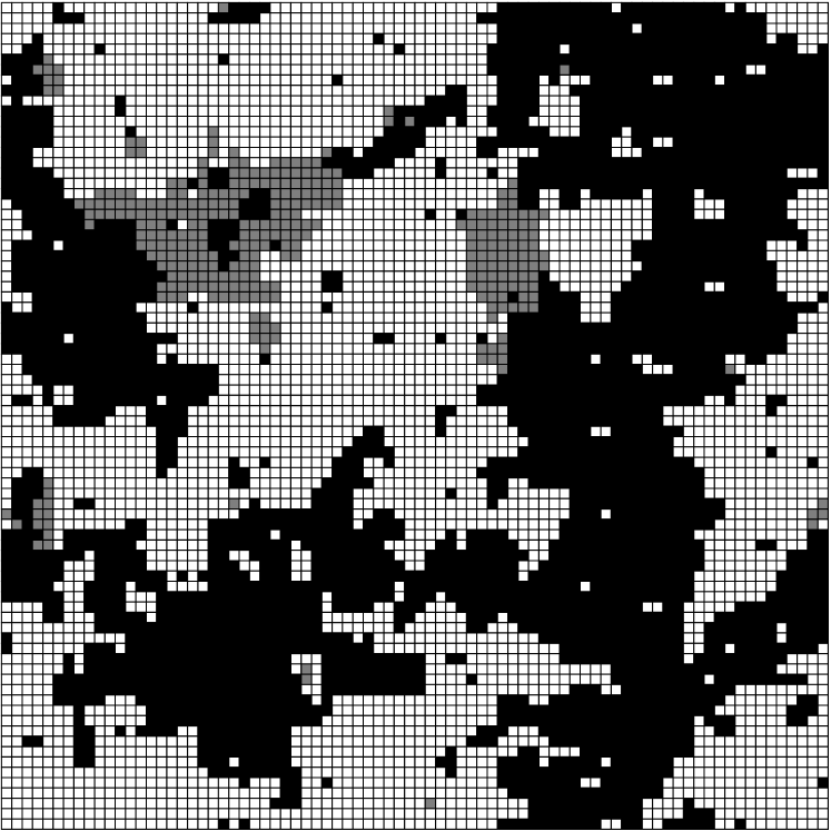
Figure 1: Two-dimensional slice through a 3d RFIM. Spins pointing $\uparrow$ are marked in white, $\downarrow$-spins in black and spins that change their orientation in the excitation in Grey.

To gather statistics, we performed simulations for systems with different $h$ at system sizes ranging from $L=10$ to $L=100$. For special values $h=2.0$, $h=2.270$, $h=2.40$ and $h=3.0$, we simulated $n=5000$ samples for each value of $L$, for the remaining values of $h$ the number of samples is dependent on the system size ($n=1000$ for the largest systems and a higher number for smaller systems).

We measured the overlap $q$ as defined in Eq. 2 where $s_{i}^{0}$ is the GS orientation of the spin at site $i$ and $s_{i}^{\prime}$ its orientation in the perturbed state. Note that $q\in[-1,1]$ independent of the system size.

We first checked whether the response of the system to the perturbation for small $\delta$ is linear. The overlap $q(\delta)$ is shown in Fig. 2. It was averaged over $5000$ samples of size $L=40$ for each $(\delta,h)$ pair. The errors are very small, due to the effect of self averaging, i.e. the total overlap does not vary strongly among different samples. For different values of $h$, and $\delta$ ranging from $\delta=.01$ to $\delta=0.5$, we found that at least until $\delta=0.2$ the relation between $q$ and $\delta$ is linear, with a slope that depends on $h$. This justified to use a fixed $\delta=0.1J$, as we did throughout our simulations.

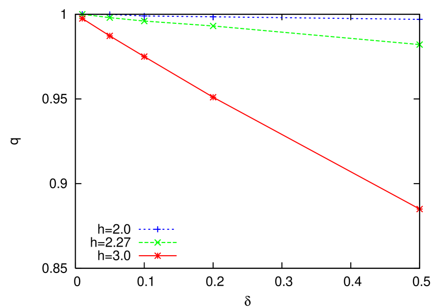
Figure 2: Overlap $q$ of the random excitations (type II) vs. perturbation strength $\delta$ for various disorder strengths $h$.

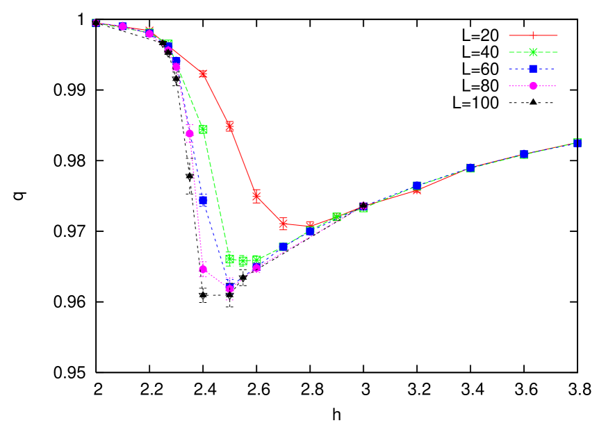
Figure 3: Dependence of the overlap $q(h)$ on the random field strength $h$ for random excitations (type II) of system sizes from $L=20$ to $L=100$. The perturbation strength is $\delta=0.1J$. The connecting lines are guides to the eyes.

In Fig. 3, the overlap $q(h)$ is shown for different values of the system size $L$. The error bars show the standard error. For large disorder strength $h$, the value of $q$ is independent of the system size and grows slowly towards $q=1$. In the limit $h\rightarrow\infty$, each spin just follows its local field independently of its neighbors, which explains this behavior.

Furthermore, one observes that close to the phase transition point $h_{c}\approx 2.27$, the overlap is smallest and changes drastically when starting from small value of $h$. The curves appear to be smooth for small sizes $L$ and significantly steeper at $L=100$. Another effect is that with growing $L$, the minimum of the overlap moves to smaller values of $q$ and closer to the phase transition $h_{c}\approx 2.27$. Thus, in the thermodynamic limit $L\to\infty$, one can expect to see a jump in $q(h)$ when approaching the phase transition from low values of the disorder $h$.

We can compare this behavior with former results of Alava and Rieger Alava98 on the two-dimensional RFIM. For any small fields $h$, the GS is paramagnetic for the two-dimensional case, in contrast three-dimensional RFIM, where the GS is ferromagneticaly ordered. Yet, the two-dimensional equivalent of Fig. 3 has a shape similar to the three-dimensional one with a “transition” to $q=1$ for small $h$. However, this apparent transition is in $d=2$ not an intrinsic property of the infinite system but a finite-size effect that is caused by the breakup length scale $L_{c}(h)$. The GSs of finite two-dimensional systems with $L<L_{c}$ are ferromagnetic since no domains can exist typically where their random-field energy exceeds their interface energy. Order is broken only for the infinite system no matter how small $h$ is, as a consequence of the argument of Imry and Ma Imry75 . Therefore, the two-dimensional transition to $q=1$ happens at some $h>0$ only in finite systems. This is reflected by the fact that for the 2d the apparent transition point shifts in two dimensions arbitrarily close to $h=0$ with growing $L$, thus it does not converge to a certain $h_{c}>0$ as our $d=3$-data suggests.

In the cited work of Alava and Rieger, the authors also make predictions as to what they expect for three dimensions. In the limits $h\to 0$ and $h\to\infty$, $q=1$ is expected. However, also for other $h$, in the thermodynamic limit $q\to 1$ is expected. These predictions are based on scaling arguments that were developed for spin glasses Bray87 and critical exponents from random-bond models nattermann1988b so that it is not clear to what extent these predictions apply to the RFIM. Our simulations rule out that at criticality and also at other values of $h$, $q\to 1$, so that only the predictions in the limit of infinite large and small $h$ are affirmed.

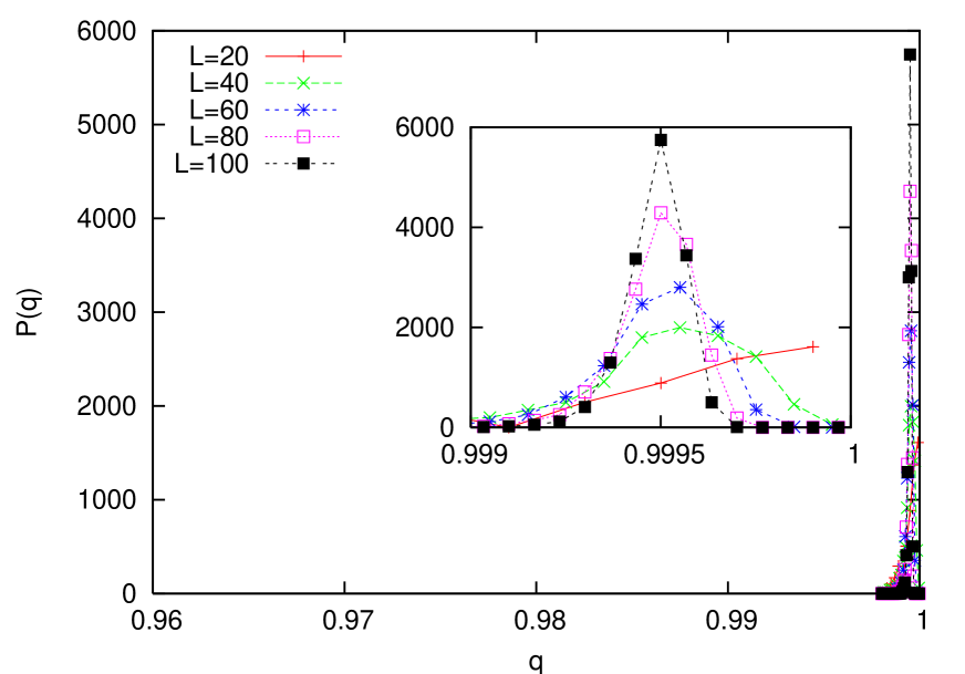
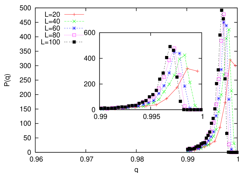
Figure 4: Histograms for the overlap distribution $P(q)$ at $h=2.0$ and $h=2.2$ for random excitations (type II) with perturbation strength $\delta=0.1J$. The distribution is sharply peaked very close to $q=1$. Therefore, a zoom to this region is shown in the respective inset. Lines are guides to the eyes only, scales are consistent with Fig. 5.

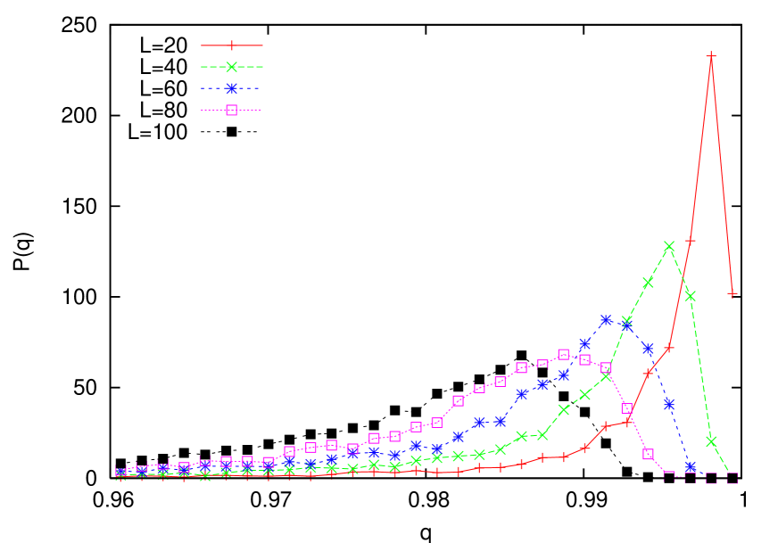
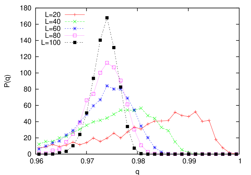
Figure 5: Histograms for the overlap distribution $P(q)$ at $h=2.4$ and $h=3.0$. Lines are guides to the eyes only.

For four selected values in the vicinity of $h_{c}\sim 2.270(4)$ HartmannYoung02 ; middleton2002 , namely $h=2.0$, $h=2.270$, $h=2.40$ and $h=3.0$, we analyzed not only the average of the overlap between ground state and excited state but also the distributions of the overlaps. The results are shown in Figs. 4. and 5. In the ferromagnetic phase, represented by $h=2.0$, there is a peak very close to $q=1$. With increasing system size, the peak becomes sharper, so that in the thermodynamic limit, $P(q)$ clearly approaches a $\delta$-shaped peak which is close to $q=0.9995$. The overlap distribution in the paramagnetic phase, represented by the $h=3.0$ plot, shows a behavior that is in some way similar. For smaller systems, there is a rather broad distribution with a maximum near $q=0.975$. The width of the distribution becomes smaller with increasing system size, and the location of the peak converges to $q\approx 0.975$. At $h=2.4$, slightly above $h_{c}$, there is a transition from the ferromagnetic peak to the onset of a developing peak at a lower $q$ that will probably become sharper for larger systems. (The maximum of the $L=80$ distribution is slightly smaller than the maximum of the $L=100$ distribution.) At the critical point with $h_{c}=2.27$, no clear statement can be made: There is a peak at $q\approx 0.996$ that resembles the ferromagnetic case, but its width stays approximately constant for the system sizes we could simulate. However, it is impossible to predict the shape of the overlap distribution in the thermodynamic limit.

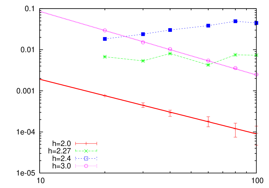
Figure 6: Dependence of the standard deviations $\delta q$ of the overlap probability distributions of Fig. 4 on $L$ ($h=2.0,2.27,2.4,3.0$). For $h=2.0$ and $h=3.0$, the lines represent power laws, while for $h=2.27$ and $h=2.4$, the lines are guides to the eyes only.

The standard deviations $\delta q$ of the distributions that are shown in Fig. 6 support this picture. While for $h=2.0$ and $h=3.0$, the width of the distribution decreases with a power law $\delta q\sim L^{-\alpha}$ with $\alpha=1.24(4)$ ($h=2.0$) and $\alpha=1.54(3)$ ($h=3.0$), no clear tendency can be seen at the intermediate $h$. If there existed in the RFIM a complex hierarchical phase-space organization resembling the replica-symmetry broken phase of the mean-field SG, the distribution of overlaps would not diverge to a $\delta$-peak in that phase. Instead, dependent on the type of replica symmetry breaking, one would would expect a distribution that is double-peaked or even flat in the thermodynamic limit. Although we could not make final predictions for $h_{c}$, our results and previous work on the sensitive of the GS to changes of the boundary conditions middleton2002 suggest that for even larger systems for all values of $h$ a $\delta$-peaked distribution should appear.

Note that the distributions we found can be compared with overlap probability distributions of uncorrelated thermal states of the RFIM in equilibrium, as performed in Sinova01 . In that work, the authors equilibrated samples by MC simulations at a low temperature. After that, the overlap distribution between the states in equilibrium was measured. The resulting $P(q)$ distributions do resemble each other strongly, which is in principle a property of a complex phase space. Nevertheless, the system sizes that could be equilibrated in Ref. Sinova01 were too small ($L<11$) to draw solid conclusions from these results.

3.2 Fractal dimension of clusters close to $h_{c}$

Droplets that represent low-energy excitations in disordered systems often exhibit a fractal structure. For the RFIM, Middleton and Fisher middleton2002 created domain walls by comparing the GS configurations of different boundary conditions in each sample. After calculating the GS where the spins on the left and right border in $x$-direction are fixed to $\uparrow$-orientation, the GS was recalculated with the spins on the right border fixed to $\downarrow$-orientation while the spins on the left border stay fixed in $\uparrow$-orientation. This method guarantees that a domain wall is created.

The fractal surface dimension of these domain walls at $h_{c}$ was determined to be $d^{d}_{s}=2.30\pm 0.04$. Middleton and Fisher also analyzed the fractal properties of clusters as areas of equal spin orientation in the simple pure GS with the result $d^{c}_{s}=2.27\pm 0.02$.

We want to determine whether the fractal dimension of low energy excitations is compatible to these results. Theory suggests that the fractal dimensions of excited clusters and domain walls should be identical if the droplet model applies. This is indeed the case for 2d Edwards-Anderson spin glasses HartmannYoung02 . But for the RFIM, system-wide non-domain-wall excitations that are uncommon because $\theta>0$, i.e. the size of typical droplets is small and not system-spanning. Note that the fact that typical droplets are small prevents us from a direct determination of the value of $\theta$ for the droplet excitations, see next section. This is in contrast to the domain-wall excitations middleton2002 , which are always of the order of the system size. This is also in contrast to the 2d SG model, where $\theta<0$. In this case, droplets tend to be large, hence the typical length scale is also given by the system size $L$.

We return to the fractal dimension, which is determined via measuring the following three quantities, see Sec. 2: We define the volume $V$ of a droplet as the number of spins it contains. If there are “holes”, i.e. areas of non-excited spins, inside of an excitation cluster they do not contribute to $V$. The surface $A$ is defined as the number of bonds that connect a spin of the cluster with a spin that is not in the cluster. For measuring the spatial extension of a cluster, we use the radius (of gyration).

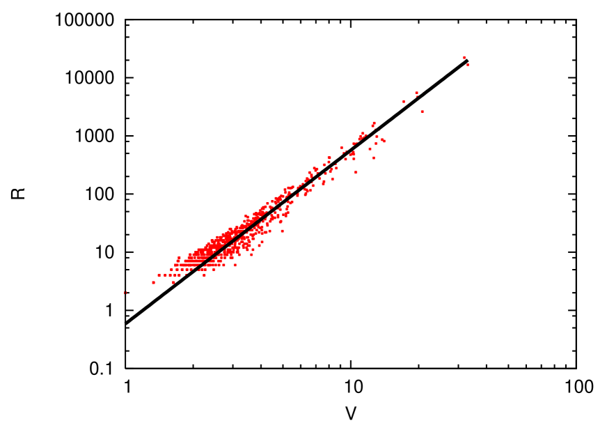
Figure 7: Volume as a function of the radius for single spin excitation clusters at $L=80$. Each data point corresponds to one cluster. A fit to the function $f(x)=ax^{b}$ yields $a=0.59(2)$ and $b=2.99(1)$, confirming $V\sim R^{3}$, as shown by the line.

As first result we obtained that the clusters are compact, i.e. the volume $V$ is non-fractal: By plotting the volume $V$ as a function of the radius of gyration $R$ for the one-spin flip method (type I) for $L=80$ ($h=h_{c}$), see Fig. 7, we find a power law with an exponent of $2.99(1)$, so that $d=3$ fits the data well. Therefore, holes inside of excited clusters are so rare and small that they do not play an important role in the excitations of the RFIM. The clusters of the other methods that were applied to calculate $d_{s}$ are compact as well (no plots shown here).

The surface scales like $A\sim R^{d_{s}}$ with the surface dimension $d_{s}$ that is possibly fractal. Combined with the compactness of the clusters, which means $V\sim R^{d}$, it follows that

$$A\sim V^{d_{s}/d}\,.$$ (5)

In Fig. 8, $A(V)$ is shown for the three different methods described above. In the double-logarithmic plot, the data of the random spin method and the $\epsilon$-coupling method is shifted by multiplying it with a factor of $10$ resp. $100$ in order to make all three curves visible in one diagram. For the pure data, the curves overlap of course. The exponent $d_{s}/d$ can be extracted from the numerical data by fitting a power law to $A(V)$.

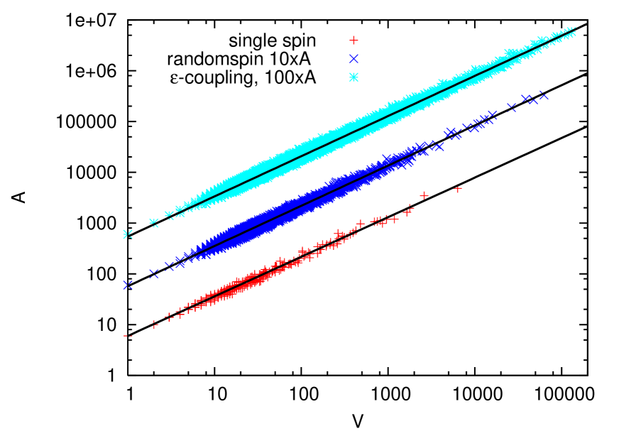
Figure 8: Excitation-cluster surface as a function of the cluster volume. for the $\epsilon$-coupling method (top), the random-excitation method (middle), and the single-spin flip method (bottom). In all three cases we observe a $A\sim V^{d_{s}/d}$ behavior (shown as lines) with $d_{s}$ being the fractal dimension, as shown in (6).

From Fig. 8, it can be seen that for the three different methods, the clusters have approximately the same fractal properties. We fitted a power law of the form $A=cV^{d_{s}/d}$ to the data of each method. The resulting fractal dimensions for each method are

$$\begin{array}[]{ll}d_{s}=2.34(2)&\mbox{single spin flip}\\ d_{s}=2.37(1)&\mbox{random excitations}\\ d_{s}=2.36(1)&\mbox{$\epsilon$-coupling}\end{array}$$ (6)

This means the three different types of excitations behave similar within error bars. Compared with the fractal dimensions calculated in middleton2002 ($d^{c}_{s}=2.27\pm 0.02$ for clusters and $d^{d}_{s}=2.3\pm 0.04$ for domain walls), our fractal dimension of small excitations is compatible with the exponent for domain walls $d^{d}_{s}$. The value for the clusters is a bit off, but this can be expected since these objects are not covered by the droplet theory. This agreement, together with the compactness of all excitation types, verifies one of the main assumptions of the droplet theory, namely that all types of physically significant excitations behave the same.

3.3 Size distributions of clusters at $h_{c}$

Another main assumption of the droplet theory fisher1988 is that the energy $\Delta E$ of minimum (free-) energy droplets with a fixed center and a given scale $l$ follows a probability distribution

$$P_{l}(\Delta E)=\frac{1}{l^{\theta}}\overline{P}(\Delta E/l^{\theta})\,,$$ (7)

where $\theta$ is the droplet-scaling exponent and $\overline{P}(.)$ is an universal function. Within the droplet theory, as already indicated above, it is assumed that the droplet exponent $\theta$ describes universally also other types of excitations, such as system-spanning domain-walls, which can be obtained numerically, as described in the previous section. Using such an approach, recently the value of $\theta=1.49(3)$ has been determined for domain walls middleton2002 .

Nevertheless, for the RFIM, we are not aware of a direct determination of the value of $\theta$ via droplet-like excitations. This is in contrast to the spin-glass case, where for the two-dimensional (2d) systems numerical simulations stiff2d ; aspect-ratio2002 ; excited2d ; droplets2003 ; droplets_long2004 indicate that domain-wall and droplet-like excitations are described by one single droplet exponent. For the 2d spin-glass case, the droplets were generated by a variant of the single-spin-flip method used in this work. Note that for 2d spin-glasses, the value of $\theta$ is negative, such that the excitations automatically tend to be as large as possible, such as to obtain an excitation energy as small as possible. Thus, in this case, the droplet scale $l$ is on average automatically given by the system size $L$.

In case the value of $\theta$ is positive, it is more difficult to determine its value via the calculation of droplet-like excitations. The reason is that size of the excitations tends to be small, as mentioned above. This means, the scale of the excitations is not given by the system size $L$, in particular each excitation will have its own scale, compatible with the minimum-energy requirement. One could use in principle a different approach to generate true droplet-like excitations, as required by the droplet theory, by optimizing only among all clusters of a given scale $l$, i.e. within a range of sizes. Nevertheless, there are no efficient optimization algorithms available, which can perform this task, in particular maximum-flow algorithms cannot be applied. It is quite likely that the problem of miniming the energy of an excitation under a size-constraint belongs even for the RFIM to the class of NP-hard problems. This means that only algorithms are known, where the running time increases in the worst case like an exponential with the system size, limiting drastically the size of tractable samples.

Therefore, we follow a different approach here: We want to use the assumption (7) to calculate the properties of the presently obtained excitations. As a first step, we want to calculate the joint probability $P(R,\Delta E;\,L)$ that, for a system size $L$, an minimum-energy excitation with fixed center exhibits the energy $\Delta E$ and has scale $R$, here as given by the radius of the excitation cluster (see Sec. 2). Since the energy of the excitation is minimum, it means that $P(R,\Delta E;\,L)$ is given by the probability that on (imaginary fixed) scale $R$ the minimum excitations energy is given by $\Delta E$ and by the probabilities that for all other scales $l\leq L$ with $l\neq R$, the excitation energy is higher. If we assume that for a fixed scale $l\leq L$ the probabilities are independent of the system size $L$, we obtain:

$$P(R,\Delta E;\,L)=P_{R}(\Delta E)\prod_{l\neq R;l\leq L}{\rm Prob}_{l}(\tilde{E}>\Delta E)$$ (8)

where ${\rm Prob}_{l}(\tilde{E}>\Delta E)$ is the probability to obtain, for a fixed center and a fixed scale $l$ a minimum-energy droplet excitation larger that $\Delta E$:

$${\rm Prob}_{l}(\tilde{E}>\Delta E) = 1-{\rm Prob}_{l}(\tilde{E}\leq\Delta E)$$ (9)

$$= 1-\int_{0}^{\Delta E}dE^{\prime}P_{l}(E^{\prime})$$

$$\stackrel{{\scriptstyle(\ref{eq:droplet:scaling})}}{{=}} 1-\int_{0}^{\Delta E}dE^{\prime}\frac{1}{l^{\theta}}\overline{P}(E^{\prime}/l^{\theta})$$

$$= 1-\int_{0}^{\Delta E/l^{\theta}}dx\overline{P}(x)$$

$$=: 1-\overline{Q}(\Delta E/l^{\theta})\,,$$

Eq. (8) can be rewritten as

$$P(R,\Delta E;\,L) = \frac{1}{R^{\theta}}\frac{\overline{P}\left(\frac{\Delta E}{R^{\theta}}\right)}{1-\overline{Q}\left(\frac{\Delta E}{R^{\theta}}\right)}\prod_{l\leq L}\left[1-\overline{Q}\left(\frac{\Delta E}{l^{\theta}}\right)\right]$$ (10)

$$= \frac{1}{R^{\theta}}\frac{\overline{P}\left(\frac{\Delta E}{R^{\theta}}\right)}{1-\overline{Q}\left(\frac{\Delta E}{R^{\theta}}\right)}e^{\sum_{l\leq L}^{\star}\ln\left[1-\overline{Q}\left(\frac{\Delta E}{l^{\theta}}\right)\right]}$$

Note that the sum $\sum_{l\leq L}^{\star}$ is performed according the assumptions of the droplet theory over different scales. Thus, it is the same as writing $l=b^{k}$ for some suitably (basically arbitrarily) chosen base $b$ and $\sum_{l\leq L}f(l)\longrightarrow\sum_{k=0}^{\log_{b}L}f(b^{k})$.

Here, using $P(R,\Delta E;\,L)$, we are interested in the distribution of excitation radii:

$$P_{L}(R):=\int_{0}^{\infty}d\Delta E\,P_{L}(R,\Delta E;\,L)\,.$$ (11)

Unfortunately, this integral over $\Delta E$ cannot be performed analytically. Nevertheless, the exponential (third) factor in (10) does not depend on $R$. Furthermore, we can assume that the factor $1/R^{\theta}$ is dominating $P_{L}(R)$, i.e. different contributions from $\Delta E/R^{\theta}$ arising in the second factor $\overline{P}/(1-\overline{Q})$ will cancel to first order. In other words, the Taylor expansion of the second term yields a constant plus higher orders in $\Delta E/R^{\theta}$. This is not unreasonable: If we consider the case of the exponential distribution, where for $\overline{P}(x)=e^{-x}$ we have $\overline{Q}(x)=1-e^{-x}$, even all contributions from $\Delta E/R^{\theta}$ cancel. In this case, just for completeness, one finally obtains, using $\lambda(L):=\sum_{k=0}^{\log_{b}L}(b^{-\theta})^{k}$ $=(1-(b^{-\theta})^{\log_{b}L+1})/(1-b^{-\theta})$ $=(1-b^{-\theta}L^{-\theta})/(1-b^{-\theta})$:

$$P_{L}(R) = \frac{1}{R^{\theta}}\int_{0}^{\infty}d\Delta Ee^{\Delta E\sum_{k}^{\star}(b^{\theta})^{k}}$$ (12)

$$= \frac{1}{R^{\theta}}\int_{0}^{\infty}d\Delta Ee^{\Delta E\lambda(L)}=\frac{1}{R^{\theta}}\frac{1}{\lambda(L)}$$ (13)

Indeed, the probabilities $P_{L}(R)$ are normalized, since $\sum_{R\leq L}^{\star}P_{L}(R)$ $=\lambda(L)\frac{1}{\lambda(L)}$ $=1$.

In Fig. 9, the measured probabilities $P_{L}(R)$ for $R>0$ are shown for single-spin-flip excitations for system with $L=80$ at the transition point $h=h_{c}$. The match with the assumed scaling form $\sim R^{-\theta}$, using $\theta=-1.49$ as obtained middleton2002 from the scaling of domain-wall energies at $h=h_{c}$, is reasonable. Also for smaller sizes $L<80$, the distribution looks similar, but they extend only to slightly smaller radii. Interestingly, for example for the $\epsilon$-coupling case the distribution shows the same power-law behavior (see inset), although the $\epsilon$-coupling excitations are not generated with a “central” spin and although each excitation generates many excitation clusters, in contrast to the assumptions used above (for the third type of excitations, the statistics is not as good right at $h_{c}$.)

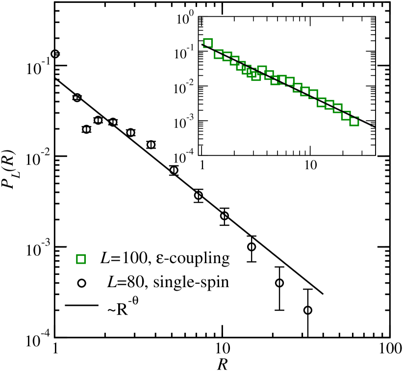
Figure 9: Probabilities $P_{L}(R)$ of cluster radii $R$ for single-spin-flips at $h=h_{c}$, the inset shows the same quantity for excitations generated by the $\epsilon$-coupling approach. Note that the probabilities are measured (i.e. integrated) over logarithmic scales, in accordance with the droplet definition within the droplet theory. The solid lines show the power laws $P(R)\sim R^{-\theta}$, which can be expected for single-spin-flip excitations (see text).

The results show that the behavior of the 3d RFIM excitations, where $\theta>0$ right at $h=h_{c}$, follow reasonably well the assumptions of the droplet-scaling theory, similar to the case of 2d spin glasses, which is an example for a system with $\theta<0$, hence simpler to treat. This result provides another strong indication that the behavior of the RFIM at the phase transition is indeed described to a large extend by the droplet theory.

4 Summary

In this paper we studied the properties of low-energy excitations in the three-dimensional RFIM via GS calculations and subsequent generation of GSs for perturbed systems. By tracking the difference of the excited state with respect to the GS of the unperturbed system, we found that the overlap $q$ undergoes a transition from $q=1$ to a smaller value that becomes steeper with growing sample size. The finite-size behavior of the data is compatible with a convergence of a drastic change of the overlap right at the critical value $h_{c}$. This constitutes a clear difference to the 2d RFIM that was analyzed by Alava and Rieger.

In the distributions $P(q)$, the phase transition is also visible in the form of a shifting peak. We did not find any clear evidence of an interval of the disorder parameter $h$ where the distribution would reach anything but a peak in the limit of infinite systems. Close to the transition $h=h_{c}$ our system sizes of even up to $L=100$ are probably too small to reach the scaling regime. This provides further evidence against a phase with a complex phase space, similar to replica-symmetry breaking, in particular right above the transition point.

The geometry of the excitation clusters was found to be compact (volume to radius) and fractal (volume to surface). Depending on the method by which the excitations were generated, the fractal dimension $d_{s}$ is slightly compared to domain walls, but not statistically significant. Furthermore the probabilities of the excitation cluster radii follow a power-law behavior $~{}R^{-\theta}$, with $\theta$ being the droplet-scaling exponent measured previously for domain walls at the phase transition point. This means that two main assumptions of the droplet theory, compactness and universality of the excitations, are verified by our results.

For future work, it would be desirable to test whether the main assumptions of the droplet theory hold also for the four-dimensional RFIM, where also some GS results have been obtained previously rfim4d2002 . Furthermore it would be desirable to study the dynamics of the RFIM within the droplet pictures, for example the scaling of energy barriers with system sizes.

- [1] Y. Imry and S.-K. Ma. Random-field instability of the ordered state of continuous symmetry. Phys. Rev. Lett., 35:1399, 1975.
- [2] M. Mézard, G. Parisi, and M.A. Virasoro. Spin glass theory and beyond. World Scientific, Singapore, 1987.
- [3] K. H. Fischer and J. A. Hertz. Spin Glasses. Cambridge University Press, Cambridge, 1991.
- [4] A. P. Young, editor. Spin glasses and random fields. World Scientific, Singapore, 1998.
- [5] S. Sabhapandit, D. Dhar, and P. Shukla. Hysteresis in the random-field ising model and bootstrap percolation. Phys. Rev. Lett., 88(19):197202, Apr 2002.
- [6] A. Rosas and S. Coutinho. Random-field Ising model on hierarchical lattices: thermodynamics and ground-state critical properties. Physica A, 335(1-2):115–142, APR 1 2004.
- [7] F. Ye, M. Matsuda, S. Katano, H. Yoshizawa, DP D.P. Belanger, E. T. Seppala, J. A. Fernandez-Baca, and MJ M. J. Alava. Percolation fractal dimension in scattering line shapes of the random-field Ising model. J. Magn. Magn. Mat., 272-76(Part 2 Sp. Iss. SI):1298–1299, MAY 2004.
- [8] F. Colaiori, M. J. Alava, G .Durin, A. Magni, and S. Zapperi. Phase transitions in a disordered system in and out of equilibrium. Phys. Rev. Lett., 92(25), JUN 25 2004.
- [9] A. Glaser, A. C. Jones, and P. M. Duxbury. Domain states in the zero-temperature diluted antiferromagnet in an applied field. Phys. Rev. B, 71(17), MAY 2005.
- [10] Markus Müller and Alessandro Silva. Instanton analysis of hysteresis in the three-dimensional random-field ising model. Phys. Rev. Lett., 96(11):117202, 2006.
- [11] D. J. Spasojevic, S. Janicevic, and M. Knezevic. Exact results for mean-field zero-temperature random-field Ising model. Europhys. Lett., 76(5):912–918, DEC 2006.
- [12] S. H. Lee, H. Jeong, and J. D. Noh. Random field ising model on networks with inhomogeneous connections. Phys. Rev. E, 74(3):031118, 2006.
- [13] Douglas F. de Albuquerque, I. P. Fittipaldi, and J. R. de Sousa. Absence of tricritical behavior of the random field Ising model in a honyecomb lattice. J. Magn. Mag. Mat., 306(1):92–97, NOV 1 2006.
- [14] V. S. Dotsenko. On the nature of the phase transition in the three-dimensional random field Ising model. S. Stat. Mech., SEP 2007.
- [15] D. M. Silevitch, D. Bitko, J. Brooke, S. Ghosh, G. Aeppli, and T. F. Rosenbaum. A ferromagnet in a continuously tunable random field. Nature, 448(7153):567–570, AUG 2 2007.
- [16] László Környei and Ferenc Iglói. Geometrical clusters in two-dimensional random-field Ising models. Phys. Rev. E, 75(1):011131, 2007.
- [17] J. J. Moreno, H. G. Katzgraber, and AK A. K.Hartmann. Finding low-temperature states with parallel tempering, simulated annealing and simple Monte Carlo. Int. J. Mod. Phys. C, 14(3):285–302, MAR 2003.
- [18] A. Magni and V. Basso. Study of metastable states in the random-field Ising model. J. Magn. Magn. Mat., 290(Part 1 Sp. Iss. SI):460–463, APR 2005.
- [19] Y. Wu and J. Machta. Ground states and thermal states of the random field Ising model. Phys. Rev. Lett., 95(13), SEP 23 2005.
- [20] V. V. Prudnikov and V. N. Borodikhin. Monte Carlo simulation of a random-field Ising antiferromagnet. J. Exp. Theor. Phys., 101(2):294–298, 2005.
- [21] Y. Wu and J. Machta. Numerical study of the three-dimensional random-field Ising model at zero and positive temperature. Phys. Rev. B, 74(6), AUG 2006.
- [22] L. Hern ndez and H. Ceva. Wang-landau study of the critical behavior of the bimodal 3d random field ising model. Physica A, 387(12):2793 – 2801, 2008.
- [23] N. G. Fytas and A. Malakis. Phase diagram of the 3D bimodal random-field Ising model. Eur. Phys. J. B, 61(1):111–120, JAN 2008.
- [24] A.K. Hartmann, A.P. Young. Large-Scale, Low-Energy Excitations in the Two-Dimensional Ising Spin Glass. Phys. Rev. B, 66:094419, 2002.
- [25] A. Alan Middleton and Daniel S. Fisher. Three-dimensional random-field ising magnet: Interfaces, scaling, and the nature of states. Phys. Rev. B, 65(13):134411, Mar 2002.
- [26] E. T. Seppälä, A. M. Pulkkinen, and M. J. Alava. Percolation in three-dimensional random field ising magnets. Phys. Rev. B, 66(14):144403, Oct 2002.
- [27] Alexander K. Hartmann. Critical exponents of four-dimensional random-field ising systems. Phys. Rev. B, 65(17):174427, May 2002.
- [28] I. Dukovski and J. Machta. Ground-state numerical study of the three-dimensional random-field Ising model. Phys. Rev. B, 67(1):014413, Jan 2003.
- [29] T. Hamasaki and H. Nishimori. Exact ground-state energies of the random-field Ising chain and ladder. J. Phys. Soc. Japan, 73(6):1490–1495, JUN 2004.
- [30] M. J. Alava, V. Basso, F. Colaiori, L. Dante, G. Durin, A. Magni, and S. Zapperi. Ground-state optimization and hysteretic demagnetization: The random-field Ising model. Phys. Rev. B, 71(6), FEB 2005.
- [31] T. Hamasaki and H. Nishimori. Exact ground-state energies of the random-field Ising chain and ladder. Progr. Theor. Phys. Suppl., 157:120–123, 2005.
- [32] M. Sarjala, V. Petaja, and M. Alava. Optimization in random field Ising models by quantum annealing. J. Stat. Mech., JAN 2006.
- [33] S. W. Son, H. Jeong, and J. D. Noh. Random field Ising model and community structure in complex networks. Eur. Phys. J. B, 50(3):431–437, APR 2006.
- [34] G. E. Santoro and E. Tosatti. Optimization using quantum mechanics: quantum annealing through adiabatic evolution. J. Phys. A, 39(36):R393–R431, SEP 8 2006.
- [35] Yang Liu and Karin A. Dahmen. No-passing rule in the ground state evolution of the random-field Ising model. Phys. Rev. E, 76(3, Part 1), SEP 2007.
- [36] M. B. Hastings. Inference from matrix products: A heuristic spin-glass algorithm. Physical Review Letters, 101(16):167206, 2008.
- [37] M. Zumsande, M. J. Alava, and A. K. Hartmann. First excitations in two- and three-dimensional random-field ising systems. J. Stat. Mech., page P02012, 2008.
- [38] W. L. McMillan. Scaling theory of Ising spin glasses. J. Phys. C, 17:3179, 1984.
- [39] A. J. Bray and M. A. Moore. Scaling theory of the ordered phase of spin glasses. In J. L. van Hemmen and I. Morgenstern, editors, Heidelberg Colloquium on Glassy Dynamics, page 121. Springer, Berlin, 1987.
- [40] D. S. Fisher and D. A. Huse. Ordered phase of short-range Ising spin-glasses. Phys. Rev. Lett., 56:1601, 1986.
- [41] D. S. Fisher and D. A. Huse. Equilibrium behavior of the spin-glass ordered phase. Phys. Rev. B, 38:386, 1988.
- [42] A. K. Hartmann and A. P. Young. Lower critical dimension of Ising spin glasses. Phys. Rev B, 64:180404, 2001.
- [43] A. K. Hartmann and M. A. Moore. Corrections to scaling are large for droplets in two-dimensional spin glasses. Phys. Rev. Lett., 90:12720, 2003.
- [44] A. K. Hartmann and M. A. Moore. Generating droplets in two-dimensional Ising spin glasses by using matching algorithms. Phys. Rev. B, 69:104409, 2004.
- [45] T. Jörg, J. Lukic, E. Marinari, and O. C. Martin. Strong universality and algebraic scaling in two-dimensional Ising spin glasses. Phys. Rev. Lett., 96:237205, 2006.
- [46] J. Bricomont and A. Kupiainen. Lower critical dimension of the random-fiel Ising model. Phys. Rev. Lett., 59:1829, 1987.
- [47] T. Nattermann. Theory of the Random Field Ising Model. Spin glasses and Random Fields (ed. P. Young), pages 277–298, 1998.
- [48] F. Barahona. On the computational complexity of Ising spin glass models. J. Phys. A, 15:3241–3253, 1982.
- [49] A. K. Hartmann. Practical Guide to Computer Simulations. Word Scientific, Singapore, 2009.
- [50] A. K. Hartmann and H. Rieger. Optimization Algorithms in Physics. Wiley-VCH, Weinheim, 2001.
- [51] M. Preissmann J. C. Anglès d’Auriac and A. Sebo. Optimal cuts in graphs and statistical mechanics. J. Math. and Comp. Model., 26:1, 1997.
- [52] H. Rieger. Ground state properties of frustrated systems. In J. Kertesz and I. Kondor, editors, Advances in Computer Simulation, Lecture Notes in Physics, volume 501, Heidelberg, 1998. Springer.
- [53] C. Moukarzel M. J. Alava, P. M. Duxbury and H. Rieger. Combinatorial optimization and disordered systems. In C. Domb and J.L. Lebowitz, editors, Phase transitions and Critical Phenomena, volume 18. Academic press, New York, 2001.
- [54] M.N.S. Swamy and K. Thulasiraman. Graphs, Networks and Algorithms. Wiley, New York, 1991.
- [55] J.D. Claiborne. Mathematical Preliminaries for Computer Networking. Wiley, New York, 1990.
- [56] K. Mehlhorn and St. Näher. The LEDA Platform of Combinatorial and Geometric Computing. Cambridge University Press, Cambridge, 1999.
- [57] J.-C. Picard and H.D. Ratliff. Minimum cuts and related problems. Networks, 5:357, 1975.
- [58] J.L. Träff. A heuristic for blocking flow algorithms. Eur. J. Oper. Res., 89:564, 1996.
- [59] R.E. Tarjan. Data Structures and Network Algorithms. Society for Industrial and Applied Mathematics, Philadelphia, 1983.
- [60] A. V. Goldberg and R. E. Tarjan. A new approach to the maximum-flow problem. J. ACM, 35:921, 1988.
- [61] B. Cherkassky and A. Goldberg. On implementing the push-relabel method for the maximum flow problem. Algorithmica, 19:390, 1997.
- [62] A. V. Goldberg and R. Satish. Beyond the flow decomposition barrier. J. ACM, 45:783, 1998.
- [63] A. A. Middleton. Critical slowing down in polynomial time algorithms. Phys. Rev. Lett., 88:017202, 2002.
- [64] A. T. Ogielski. Integer optimization and zero-temperature fixed point in Ising random-field systems. Phys. Rev. Lett., 57:1251, 1986.
- [65] A. K. Hartmann and U. Nowak. Universality in three dimensional random field systems. Eur. Phys. J. B, 7:105, 1999.
- [66] The RFIM with a delta-distribution of the random fields () exhibits an exponential ground-state degeneracy.
- [67] J.-C. Picard and M. Queyranne. On the structure of all minimum cuts in a network and applications. Math. Prog. Study, 13:8, 1980.
- [68] A. K. Hartmann. Ground state structure of diluted antiferromagnets and random field systems,. Physica A, 248:1, 1998.
- [69] S. Bastea and P. M. Duxbury. Ground state structure of random magnets. Phys. Rev. E, 58:4261, 1998.
- [70] M. Alava, H. Rieger. Chaos in the random field Ising model. Phys. Rev. E, 58:4284, 1998.
- [71] D. Fisher, A. Huse. Nonequilibrium dynamics of spin glasses. Phys. Rev. B, 38:373–385, 1988.
- [72] A. J. Bray, M.A. Moore. Chaotic Nature of the Spin-Glass Phase . Phys. Rev. Lett., 58:57–60, 1987.
- [73] Y. Imry, S. Ma. Random-Field Instability of the Ordered State of Continous Symmetry. Phys. Rev. Lett., 35:1399–1401, 1975.
- [74] T. Nattermann. Ground-state instability of interfaces in random-systems. Phys. Rev. Lett., 60(25):2701, jun 20 1988.
- [75] J. Sinova and G. Canright. Nature and number of distinct phases in the random-field Ising model. Phys. Rev. B, 64:094402, 2001.
- [76] A. K. Hartmann, A. J. Bray, A. C. Carter, M. A. Moore, and A. P. Young. The stiffness exponent of two-dimensional Ising spin glasses for non-periodic boundary conditions using aspect-ratio scaling. Phys. Rev. B, 66:224401, 2002.
- [77] A. K. Hartmann and A. P. Young. Large-scale, low-energy excitations in the two-dimensional Ising spin glass. Phys. Rev B, 65:094419, 2002.