Locally stationary long memory estimation

Abstract.

There exists a wide literature on parametrically or semi-parametrically modeling strongly dependent time series using a long-memory parameter $d$, including more recent work on wavelet estimation. As a generalization of these latter approaches, in this work we allow the long-memory parameter $d$ to be varying over time. We adopt a semi-parametric approach in order to avoid fitting a time-varying parametric model, such as tvARFIMA, to the observed data. We study the asymptotic behavior of a local log-regression wavelet estimator of the time-dependent $d$. Both simulations and a real data example complete our work on providing a fairly general approach.

1. Introduction

There is a long tradition of modelling the phenomenon of long-range dependence in observed data that show a strong persistence of their correlations by long-memory processes. Such data can typically be found in the applied sciences such as hydrology, geophysics, climatology and telecommunication (e.g. teletraffic data) but recently also in economics and in finance, e.g. for modelling (realized) volatility of exchange rate data or stocks. The literature on stationary long-memory processes is huge (see e.g. the references in the recent survey paper [13]), and we concentrate here on the discussion of long-range dependence resulting from a singularity of the spectral density at zero frequency - corresponding to a slow, i.e. polynomial, decay of the autocorrelation of the data. Although a lot of (earlier) work started from a parametric approach, using e.g. the celebrated ARFIMA-like models, it occurs that since the seminal work by P. Robinson (see [25, 26]), the semi-parametric approach is known to be more robust against model misspecification: instead of using a parametric filter describing both the singularity of the spectral density at zero frequency and the ARMA-dynamics of the short memory part, only the singular behavior of the spectrum at zero is modelled by the long-memory parameter, $d$ say, whereas the short memory part remains completely non-parametric.

Driven by the empirical observation that the correlation structure of observed (weakly or strongly dependent) data can change over time, there is a also a growing literature on modelling departures from covariance-stationarity, mainly restricted to the short-range dependent case. One prominent approach, that we adopt in this paper, too, is the model of local stationarity, introduced by a series of papers by R. Dahlhaus ([4, 5, 6]): in a non-parametric set-up, the spectral structure of the underlying stochastic process is allowed to be smoothly varying over time. Of course, time-varying linear processes (of ARMA type) arise as a subclass of these locally stationary processes. In order to come up with a rigorous asymptotic theory of consistency and inference, the time-dependence of the spectral density $f(u,\lambda)$ of such locally stationary processes is modelled to be in rescaled time $u\ \in[0,1]$, leading to a problem of non-parametric curve estimation: increasing the sample size $T$ of the observed time series does no more mean to look into the future but to dispose of more and more observations to identify $f(t/T,\lambda)$ locally around the “reference” rescaled time point $u\approx t/T$.

In the aforementioned spirit of semi-parametric modelling, and in contrast to the parametric approach of [3], one of the very few existing approaches on time-varying long-memory modelling, we consider in this paper a locally stationary long-range dependent process with a singularity in the spectral density at zero frequency which is parameterized by a time-varying long-memory parameter $d=d(u)$, $u\in[0,1]$, i.e. defined in rescaled time. Our approach is a true generalization of the stationary approach in that the latter corresponds to a time-constant $d$ for our locally stationary model. As in the case of [23], the long memory parameter is estimated by a log-regression of a series of wavelet scalograms (estimated wavelet variances per scale by summing the squared wavelet coefficients per scale over location) onto a range of scales (corresponding to the low frequency range of the spectrum). Although wavelets do not improve the estimation of $d$ in the standard stationary context $-1/2<d<1/2$, their use is of interest in various practical situations (presence of trends, under and over-differenced series leading to $d\geq 1/2$ and $d\leq-1/2$ respectively), see details in [13]. However, in our work now the challenge is to localize the estimation of the no more constant parameter $d$. Wavelets are favorable in this situation since, in contrast to a Fourier analysis, they are well localized both over time and frequency, i.e. scale. The localization is achieved by smoothing over time the series of squared wavelet coefficients on each of the coarse scales which enter into the log-regression, giving raise to a local scalogram. We propose both a more traditional method based on two-sided kernels and also a recursive scheme of one-sided smoothing weights, adapted to the end point of the observation period.

The model studied in this paper arises naturally in the now long history of time series modelling in presence of persistent memory. A survey on this subject is provided in [30]. In Chapter 3 of this reference, it is recalled how long memory and non stationarity have been used as concurrent modelling approaches, in particular for financial data, see e.g. [19]. Long memory modeling for financial data goes back to [12]. Originally investigated on absolute powers of stock returns, long memory models are currently widely used for realized volatility data since they were proven efficient for forecasting purposes in this context in [2]. It is interesting to note that only 3 years after [12], the need for time varying long memory parameters was pointed out in [11], see Section 5 and in particular Figure 6 where an estimated $d$ is plotted evolving between the values $0.358$ and $0.714$ over a 60 years long period. In this reference two approaches are suggested for coping with a time varying $d$, namely, a stochastically evolving $d$ or a regime switching between, say, two values of $d$. These two approaches have been developed, respectively, in [24] and [17] (see also [16] where singularities in the spectral density at frequencies different from zero are considered in a piecewise stationary context).

As outlined earlier the alternative approach developed by Dahlhaus for locally stationary (short memory) processes is quite appealing as it allows a meaningful asymptotic study of the estimators. It was recently used for volatility estimation using time varying (short memory) non-linear processes, see [9, 15]. The first attempt to adapt Dahlhaus’s approach in the presence of long memory appears to be the unpublished preprint [18]. The authors use the log linear relationship of the local variance of the maximum overlap discrete wavelet transform and their scaling parameter, plus a localization with a rectangular window in coefficient domain, to estimate the time-varying long memory parameter. However, the asymptotic analysis of the proposed estimator is not provided. Although it is not essential in their analysis, the considered model is a tvARFIMA$(q,d,r)$, see our examples below. An asymptotic analysis is provided in [3] for a different estimator applied to the same model. Roughly speaking, the standard way to estimate a time varying parameter $d(u)$ at rescaled time $u=t/T\in(0,1)$ of a locally stationary process is to use that, for a sample size $T$, $Tb$ observations around time index $t$ approximately behave as a stationary sample as the bandwidth parameter $b\to 0$. In [3, Theorems 1] the proposed estimator of the time varying long memory parameter $d$ is claimed to satisfy a central limit theorem at rate $(Tb)^{-1/2}$. On the other hand Theorem 2 in [3] says that the bias is of order $b^{2}$ if $d$ is two times continuously differentiable. Such results are somewhat similar to that for estimating the time varying parameter of a locally stationary short memory process, see [20], or, in a more general fashion, Example 3.6 in [7]. Hence the presence of long memory in [3] seems not to affect the estimation rates. It can be explained by the parametric approach for the correlation structure of the observed locally stationary time series in that the filter in the linear (although infinite) locally autoregressive representation of the process is completely determined by a finite-dimensional parameter. It follows that only a finite number of local correlations are needed to determine the local parameter $d$. In other words the estimation of $d(u)$ can be obtained from an analysis over a fixed set of frequencies taken away from zero. This would however induce a high sensitivity to model misspecification. In contrast, as usual in semi-parametric vs parametric estimation, we want our approach to be robust against model misspecification. To impose this robustness in the semi-parametric model, the memory parameter $d$ is disconnected from the spectral content out of the origin so that short range correlations does not carry any information about this parameter. This fully justifies the semi-parametric context even though it is more involved as it necessitates a low frequency analysis (where the long memory behavior occurs) which, at first sight, seems contradictory to the local stationarity framework. In fact, this contradiction is inherent to any locally stationary model which rely on a compromise between stationarity, which appears at small scales, and analyzing bandwidth, which requires a large scale to decrease the randomness in the data. As a consequence practical applications of these models require very long data sets. Our results will prove that this apparent contradiction can still be overcome for locally stationary long memory models, but with some price to pay on the rate of estimation (although we are unable to prove that this price is optimal). It is not as surprising as it may appear. To understand why, consider a piecewise stationary context where a finite number of regime switching times occur over the observation sample. One clearly sees that the long memory over each stationary segment can be estimated at the same rate as in the stationary context. As we will see, the picture is more complicated in a locally stationary context but it can still be handled. More precisely, we will show that looking at low frequencies is allowed in a locally stationary model but with an additional cost on the rate of convergence depending on how small the frequency used for the analysis is. We believe that such theoretical results are crucial for the practical estimation of the time varying long memory parameter as they demonstrate the viability of such an approach while indicating that it should be applied with care.

Summarizing our results, the rest of the paper is organized as follows. In Section 2, we give the technical details of our locally stationary long memory model of semi-parametric type and give a series of examples of processes falling into this model. In Section 3 we define our estimators based on wavelet analysis for which we briefly recall the wavelet set-up. We define the local scalogram which is at the heart of our wavelet based estimators. We also prepare our technique of stationary approximation by defining what we call the approximating stationary tangent process and its wavelet spectrum, the local wavelet spectrum, as well as the pseudo-estimator tangent scalogram. We finish this section by discussing a series of smoothing weights, one- and two-sided kernels, which fulfill our given assumptions. The asymptotic properties of our proposed estimators are stated in the following Section 4. We derive a mean-square approximation of the local scalogram through the tangent scalogram (Proposition 1), followed by a control of the mean square error of the scalogram as an estimator of the local wavelet spectrum (Theorem 1) and a CLT for the tangent scalogram (Theorem 2), which finally allows us to derive a CLT for the local scalogram (Corollary 1). The results on the asymptotic behavior of the estimator of $d(u)$ are then obtained: Corollary 2 provides the rate of convergence and Theorem 3 the asymptotic normality. We pursue the paper by Section 5 on numerical examples, first simulating some ARFIMA process with a time-varying $d$ and comparing the performance of the two-sided (rectangular) kernel with the recursive weight scheme. Second, we apply the kernel estimator to a series of realized log volatilities (see also [31]), namely of the exchange rate of the YEN versus USD, from June 1986 to September 2004. We conclude in Section 6 before an appendix section presents all technical details of our derivations including our proofs.

2. Model set-up and examples

Define the difference operator $[\mathbf{\Delta}X]_{k}=X_{k}-X_{k-1}$ and $\mathbf{\Delta}^{p}$ recursively. This will allow $d(u)$ to take values up to $p+1/2$ in the following model.

We adapt the approach of [4] to the case where the spectral density is allowed to have a singularity at the zero frequency. Let us fix $p=0,1,2,\dots$ and $A^{0}_{t,T}(\lambda)$ be an array of $L^{2}([-\pi,\pi])$ functions with real-valued Fourier coefficients. Let $\{X_{t,T}\}$ be an array of real-valued random variables such that

$$\mathbf{\Delta}^{p}X_{t,T}=\int_{-\pi}^{\pi}A^{0}_{t,T}(\lambda)\ \mathrm{e}^{\mathrm{i}\lambda t}\;\mathrm{d}Z(\lambda)\ ,\qquad t=1,\ldots T,\ T\geq 1\ ,$$ (1)

where $\mathrm{d}Z(\lambda)$ is the spectral representation of a centered weak white noise with unit variance,

$$\varepsilon_{t}=\int_{-\pi}^{\pi}\mathrm{e}^{\mathrm{i}\lambda t}\;\mathrm{d}Z(\lambda),\quad t\in\mathbb{Z}\;,$$ (2)

hence $Z(\lambda)$ is a Hermitian complex valued process with weakly stationary orthogonal increments on $[-\pi,\pi]$. We further assume that there exist a function $A(u,\lambda)$ in $L^{2}([0,1]\times[-\pi,\pi])$ and two constants $c>0$ and $D<1/2$ such that

$$\left|A^{0}_{t,T}(\lambda)-A(t/T,\lambda)\right|\leq c\;T^{-1}\;|\lambda|^{-D}\,,\quad 1\leq t\leq T,\,-\pi\leq\lambda\leq\pi\;,$$ (3)

and

$$\left|A(u;\lambda)-A(v,\lambda)\right|\leq c\;|v-u|\;|\lambda|^{-D}\,,\quad 0\leq u,v\leq 1,\,-\pi\leq\lambda\leq\pi\;.$$ (4)

These correspond to the definition of locally stationary processes introduced in [4] but with the term $|\lambda|^{-D}$ added in the upper bound to allow a singularity at the zero frequency. Relations (1), (3) and (4) give rise to the following time-varying generalized spectral density of $\{X_{t,T}\}$

$$f(u,\lambda)=|1-\mathrm{e}^{-\mathrm{i}\lambda}|^{-2p}\;\left|A(u;\lambda)\right|^{2}\;.$$ (5)

The first multiplicative factor in the right-hand side of (5) corresponds to the operator $\mathbf{\Delta}^{p}$ in the left-hand side of (1). We now focus on time-varying generalized spectral densities exhibiting a memory parameter at zero frequency.

Definition 1.

We say that the process $\{X_{t,T},\;t=1,\ldots,T,\ T\geq 1\}$ has local memory parameter $d(u)\in(-\infty,p+1/2)$ at time $u\in[0,1]$ if it satisfies (1), (3) and (4) and its generalized spectral density $f(u,\lambda)$ defined by (5) satisfies the following semi-parametric type condition:

$$f(u,\lambda)=|1-\mathrm{e}^{-\mathrm{i}\lambda}|^{-2d(u)}\ f^{*}(u,\lambda)\ ,$$ (6)

with $f^{*}(u,0)>0$ and

$$|f^{*}(u,\lambda)-f^{*}(u,0)|\leq C\;f^{*}(u,0)\;|\lambda|^{\beta},\;\lambda\in[-\pi,\pi]\;,$$ (7)

where $C>0$ and $\beta\in(0,2]$.

The assumption on the model is summarized hereafter.

Assumption 1.

The array $\{X_{t,T}\}$ of real-valued random variables has local memory parameter $d(u)\in(-\infty,p+1/2)$ at time $u\in[0,1]$. Moreover $\{\varepsilon_{t}\}$ in (2) is a weak white noise such that $\mathbb{E}[\varepsilon_{0}]=0$, $\mathrm{Var}(\varepsilon_{0})=1$, $\mathbb{E}[\varepsilon_{t}^{4}]$ is finite for all $t\in\mathbb{Z}$ and the fourth-order cumulants of its spectral representation $\mathrm{d}Z(\lambda)$ satisfy

$$\mathrm{Cum}\left(\mathrm{d}Z(\lambda_{k}),\,1\leq k\leq 4\right)=\hat{\kappa}_{4}(\lambda)\;\mathrm{d}\mu(\lambda),\quad\lambda=(\lambda_{k})_{1\leq k\leq 4}\in[-\pi,\pi]^{4}\;,$$ (8)

where $\hat{\kappa}_{4}(\lambda)=\hat{\kappa}_{4}(\lambda_{1},\lambda_{2},\lambda_{3})$ is a bounded function defined on $[-\pi,\pi]^{3}$, and $\mu$ is defined as the measure on $[-\pi,\pi]^{4}$ such that, for any $(2\pi)$-periodic functions $A_{k}$, $1\leq k\leq 4$,

$$\int_{[-\pi,\pi]^{4}}\prod_{k=1}^{4}A_{k}(\lambda_{k})\;\mathrm{d}\mu(\lambda)=\int_{[-\pi,\pi]^{3}}A_{4}(-\lambda_{1}-\lambda_{2}-\lambda_{3})\,\prod_{k=1}^{3}A_{k}(\lambda_{k})\;\mathrm{d}\lambda\;.$$ (9)

Assumption (8) is standard for linear representations of time series and was used by Dahlhaus (for cumulants of all orders) in the original definition of locally stationary processes in [5]. The measure $\mu$ defined by (9) is sometimes denoted as $\mathrm{d}\mu(\lambda)=\eta(\lambda_{1}+\dots+\lambda_{4})\mathrm{d}\lambda_{1}\dots\mathrm{d}\lambda_{4}$, where $\eta$ is the $(2\pi)$-periodic Dirac comb, see e.g. [5, 8]. An immediate consequence of (8) is the following bound of fourth-order cumulants, for any set of $(2\pi)$-periodic functions $A_{k}$, $1\leq k\leq 4$,

$$\left|\mathrm{Cum}\left(\int_{-\pi}^{\pi}A_{k}(\lambda)\mathrm{d}Z(\lambda),\,1\leq k\leq 4\right)\right|\leq c_{4}\;\|A_{1}\|_{2}\,\|A_{4}\|_{2}\,\|A_{2}\|_{1}\|A_{3}\|_{1}\;,$$ (10)

where $c_{4}$ is a positive constant and $\|A_{k}\|_{p}=(\int_{-\pi}^{\pi}|A_{k}(\lambda)|^{p}\mathrm{d}\lambda)^{1/p}$.

We now give a small series of examples, adapted from [23] to the time varying setting.

Example 1 (tvFBM($H$)).

The Fractional Brownian motion (FBM) process $\{B_{H}(k)\}_{k\in\mathbb{Z}}$ with Hurst index $H\in(0,1)$ is a discrete-time version of $\{B_{H}(t),t\in\mathbb{R}\}$, a Gaussian process with mean zero and covariance

$$\mathbb{E}[B_{H}(t)B_{H}(s)]=\frac{1}{2}\left\{|t|^{2H}+|s|^{2H}-|t-s|^{2H}\right\}\;.$$

The spectral density of $\{\mathbf{\Delta}B_{H}(k)\}_{k\in\mathbb{Z}}$ is then given by $\lambda\mapsto|1-\mathrm{e}^{-\mathrm{i}\lambda}|^{-2H+1}f_{\mathrm{FBM}}(\lambda;H)$, where

$$f_{\mathrm{FBM}}(\lambda;H)=\left|\frac{2\sin(\lambda/2)}{\lambda}\right|^{2H+1}+\left|2\sin(\lambda/2)\right|^{2H+1}\sum_{k\neq 0}\left|\lambda+2k\pi\right|^{-2H-1}\;.$$ (11)

The time varying Fractional Brownian motion (tvFBM) has generalized spectral density (6) with $p=1$, $d(u)=H(u)+1/2\in(1/2,3/2)$ and $f^{\ast}(u,\lambda)=f_{\mathrm{FBM}}(\lambda;H(u))$, where $H$ is a Lipschitz mapping of $[0,1]$ into a subset of $(0,1)$. Then (7) holds with $\beta=(2H(u)+1)\wedge 2$. The corresponding non-negative local transfer function is

$$A(u,\lambda)=|1-\mathrm{e}^{-\mathrm{i}\lambda}|^{1/2-H(u)}\sqrt{f_{\mathrm{FBM}}(\lambda;H(u))}\;.$$ (12)

In this case, by Lemma 3 in B, (4) holds for any $D>\sup_{u}H(u)-1/2$.

Example 2 (tvFGN($H$)).

The time varying fractional Gaussian noise (tvFGN) is defined similarly as the tvFBM by $f^{\ast}(u,\lambda)=f_{\mathrm{FBM}}(\lambda;H(u))$ but with $p=0$ and $d(u)=H(u)-1/2\in(-1/2,1/2)$.

Example 3 (approximated causal tvFBM($H$)).

The drawback of the tvFBM (and also of tvFGN) defined above is the non-causality of the transfer function $A(u,\cdot)$ defined in (12). Since $\{\mathbf{\Delta}B_{H}(k)\}_{k\in\mathbb{Z}}$ is purely non-deterministic, it admits a causal representation. On the other hand, to our knowledge, the corresponding transfer function is not explicitly given and thus (4) is difficult to check. To circumvent this problem, one may construct an example by approximating a causal continuous time representation of the FBM, see e.g. [30, Chapter 6]. Let us fix $H$ in $(1/2,1)$. Replacing the integral by a discrete sum in this representation, one obtains the following process

$$\tilde{B}_{H}(t)=\sum_{s\in\mathbb{Z}}\{(t-s)_{+}^{H-1/2}-(-s)_{+}^{H-1/2}\}\,\varepsilon_{s},\quad t\in\mathbb{Z}\;,$$

where $\{\varepsilon_{s}\}_{s\in\mathbb{Z}}$ is a standard Gaussian white noise. Then

$$\mathbf{\Delta}\tilde{B}_{H}(t)=\sum_{k\geq 0}\{k^{H-1/2}-(k-1)_{+}^{H-1/2}\}\,\varepsilon_{t-k},\quad t\in\mathbb{Z}\;,$$

is a causal representation of a stationary process. Using an integral approximation of the discrete Fourier transform of the sequence $(k_{+}^{H-1/2}-(k-1)_{+}^{H-1/2})_{k\in\mathbb{Z}}$, one can show that, as $\lambda\to 0$, the corresponding transfer function $A_{H}(\lambda)$ satisfies $|A_{H}(\lambda)|=C_{H}\,|\lambda|^{1/2-H}+O(1)$ for some positive constant $C_{H}$. Moreover, for any $\epsilon>0$, there is a constant $C$ such that, for all $1/2<H^{\prime}\leq H<1$ and $\lambda\in(-\pi,\pi)$,

$$|A_{H}(\lambda)-A_{H^{\prime}}(\lambda)|\leq C\,|H-H^{\prime}|\,|\lambda|^{H-1/2-\epsilon}\;.$$

Let now $H$ be a Lipschitz mapping of $[0,1]$ into a subset of $(1/2,1)$ and define the approximated causal tvFBM($H$) process by setting $A(u,\lambda)=A_{H(u)}(\lambda)$. Then Condition (4) holds again for any $D>\sup_{u}H(u)-1/2$.

Example 4 (tvARFIMA$(q,d,r)$).

The time varying autoregressive fractionally integrated moving average (tvARFIMA$(q,d,r)$) process is defined by

$$A(u;\lambda)=(1-\mathrm{e}^{-\mathrm{i}\lambda})^{-d(u)+p}\;\frac{\sigma(u)}{\sqrt{2\pi}}\;\frac{1+\sum_{k=1}^{r}\theta_{k}(u)\mathrm{e}^{-\mathrm{i}\lambda}}{1-\sum_{k=1}^{q}\phi_{k}(u)\mathrm{e}^{-\mathrm{i}\lambda}}\;,$$ (13)

where $d:[0,1]\to(-\infty,p+1/2)$, $\sigma:[0,1]\to\mathbb{R}_{+}$, $\phi=[\phi_{1}\,\,\dots\,\,\phi_{q}]^{T}:[0,1]\to\mathbb{R}^{q}$ and $\theta=[\theta_{1}\,\,\dots\,\,\theta_{r}]^{T}:[0,1]\to\mathbb{R}^{r}$ are Lipschitz functions such that $1-\sum_{k=1}^{q}\phi_{k}(u)z^{k}$ does not vanish for all $u\in[0,1]$ and $z\in\mathbb{C}$ such that $|z|\leq 1$. Using this latter condition, the local transfer function $A(u;\cdot)$ defines a causal autoregressive fractionally integrated moving average (ARFIMA$(q,d(u)-p,r)$) process and the local generalized spectral density (5) satisfies the conditions (6) and (7) with $\beta=2$. Using Lemma 3 in B, the Lipschtiz assumptions on $d$, $\sigma$, $\theta$ and $\phi$ yield the condition (4) with $D>\sup_{u}d(u)-p$.

In order to verify Condition (3) trivially, the simplest definition of $\{\mathbf{\Delta}^{p}X_{t,T}\}$ in all the previous examples is to take $A^{0}_{t,T}(\lambda)=A(t/T,\lambda)$, that is to set the time-varying linear representation

$$\mathbf{\Delta}^{p}X_{t,T}=\int_{-\pi}^{\pi}A(t/T;\lambda)\ \mathrm{e}^{\mathrm{i}\lambda t}\;\mathrm{d}Z(\lambda)\;,$$ (14)

as will be done for our simulated tvARFIMA in Section 5. However, one might also want to use a different transfer function $A^{0}_{t,T}$ in (1), provided that Condition (3) holds. Such approximated time varying linear representation is motivated by the tvAR($p$) process, which satisfies the recursion

$$X_{t,T}-\sum_{k=1}^{p}\phi_{k}(t/T)X_{t-k,T}=\sigma(t/T)\;\varepsilon_{t},\quad 1\leq t\leq T\;,$$

along with appropriate initial conditions. It has been shown in [4] that such non-stationary process does not satisfy a representation of the form (14) (with $p=0$) but it does satisfy (1) and (3) (with $p=D=0$).

3. Estimation method based on wavelet analysis

3.1. Discrete wavelet transform (DWT)

Following the approach presented in [23] for the estimation of the memory parameter of a stationary sequence, we compute the discrete wavelet transform (DWT) of $\{X_{t,T},\;1\leq t\leq T\}$ (in discrete time) for a given scale function $\phi$ and wavelet $\psi$. We denote by $\{W_{j,k;T}\,;j\geq 0,k\in\mathbb{Z}\}$ the wavelet coefficients of the process $\{X_{t,T},\,1\leq t\leq T\}$,

$$W_{j,k;T}=\sum_{t=1}^{T}h_{j,2^{j}k-t}X_{t,T},\quad k=0,\dots,T_{j}-1\;,$$ (15)

where $\{h_{j,t},\;,t\in\mathbb{Z}\}$ denotes the wavelet detail filter at scale $j$ associated to $\phi$ and $\psi$ through the relation

$$h_{j,t}=2^{-j/2}\int_{-\infty}^{\infty}\phi(u+t)\psi(2^{-j}u)\;\mathrm{d}u\;,$$

and $T_{j}$ the number of available wavelet coefficients at scale $j$, which satisfies

$$T2^{-j}-c\leq T_{j}\leq T2^{-j},\quad\text{for some constant $c$ independent of $j\geq 0$}\;.$$ (16)

The filter $h_{j,\cdot}$ and $T_{j}$ are defined so that the support $\{t~{}:~{}h_{j,2^{j}k-t}\neq 0\}$ is included in $\{1,\dots T\}$ for $k=0,\dots,T_{j}-1$. Observe that here $j$ denotes the scale index of the wavelet coefficient and $k$ its position index. We use the convention that a large $j$ corresponds to a coarse scale. Let us define

$$H_{j}(\lambda)=\sum_{t\in\mathbb{Z}}h_{j,t}\mathrm{e}^{-\mathrm{i}t\lambda}$$ (17)

the corresponding filter transfer function. The following conditions on the wavelet $\psi$ and scale function $\phi$ are assumed to hold for a positive integer $M$ and a real $\alpha$.

1. $\phi$ and $\psi$ are compactly-supported, integrable, $\int_{-\infty}^{\infty}\phi(t)\,\mathrm{d}t=1$ and $\int_{-\infty}^{\infty}\psi^{2}(t)\,\mathrm{d}t=1$.

2. There exists $\alpha>1$ such that $\sup_{\xi\in\mathbb{R}}|\hat{\psi}(\xi)|\,(1+|\xi|)^{\alpha}<\infty$, where $\hat{\psi}(\xi)=\int_{-\infty}^{\infty}\psi(t)\,\mathrm{e}^{-\mathrm{i}\xi t}\mathrm{d}t$ denotes the Fourier transform of $\psi$.

3. The function $\psi$ has $M$ vanishing moments, $\int_{-\infty}^{\infty}t^{m}\psi(t)\,\mathrm{d}t=0$ for all $m=0,\dots,M-1$

4. The function $\sum_{k\in\mathbb{Z}}k^{m}\phi(\cdot-k)$ is a polynomial of degree $m$ for all $m=0,\dots,M-1$.

Under (W-3) and (W-4), the filter can be interpreted as the convolution of the $\mathbf{\Delta}^{M}$ filter with a finite impulse response filter. Hence if $M\geq p$, Equation (15) may be written as

$$W_{j,k;T}=\sum_{t=1}^{T}\tilde{h}_{j,2^{j}k-t}(\mathbf{\Delta}^{p}X)_{t,T},\quad k=0,\dots,T_{j}-1\;,$$

where $h_{j,\cdot}=\tilde{h}_{j,\cdot}\ast\mathbf{\Delta}^{p}$. In particular, we have

$$\tilde{H}_{j}(\lambda)=\sum_{t\in\mathbb{Z}}\tilde{h}_{j,t}\mathrm{e}^{-\mathrm{i}t\lambda}=H_{j}(\lambda)(1-\mathrm{e}^{\mathrm{i}\lambda})^{-p}\;.$$ (18)

3.2. Local wavelet spectrum, local scalogram, tangent scalogram, and final estimator

Recall that $f(u,\cdot)$ in (5) can be interpreted as a local generalized spectral density at rescaled time $u\in[0,1]$. Hence, as in the stationary setting used in [23], for each such $u$, we may define a local wavelet spectrum $\sigma^{2}(u)=\{\sigma^{2}_{j}(u),\,j\geq 0\}$, where for each $j\geq 0$, $\sigma^{2}_{j}(u)$ is the variance of the wavelet coefficients at scale index $j$ of a process with generalized spectral density $f(u,\cdot)$. This variance is well defined under the assumption $M\geq p$ because in this case the wavelet coefficients at given scale are weakly stationary. Moreover, by (5) and (18),

$$\sigma^{2}_{j}(u)=\int_{-\pi}^{\pi}\left|{H}_{j}(\lambda)\right|^{2}\,f(u;\lambda)\;\mathrm{d}\lambda=\int_{-\pi}^{\pi}\left|\tilde{H}_{j}(\lambda)\ A(u;\lambda)\right|^{2}\;\mathrm{d}\lambda\;.$$

The following intuitive definition will be also useful when developing our estimation theory using stationary approximations. For any $u\in[0,1]$ one may define a tangent stationary process for the $p$-th increment

$$\mathbf{\Delta}^{p}X_{t}(u)=\int_{-\pi}^{\pi}A(u;\lambda)\ \mathrm{e}^{\mathrm{i}\lambda t}\;\mathrm{d}Z(\lambda)\ ,$$ (19)

whose spectral density is $|1-\mathrm{e}^{-\mathrm{i}\lambda}|^{2p}f(u,\lambda)$. Further we define the wavelet coefficients of the tangent weakly stationary process at any $u\in[0,1]$, namely,

$$W_{j,k}(u) =\sum_{t=1}^{T}\tilde{h}_{j,2^{j}k-t}(\mathbf{\Delta}^{p}X)_{t}(u)$$ (20)

$$=\int_{-\pi}^{\pi}\tilde{H}_{j}(\lambda)\ A(u;\lambda)\ \mathrm{e}^{\mathrm{i}\lambda 2^{j}k}\;\mathrm{d}Z(\lambda)\;,\quad k=0,\dots,T_{j}-1\;.$$ (21)

these wavelet coefficients are indeed those of a process with generalized spectral density $f(u,\cdot)$. Thus the above definition gives

$$\sigma^{2}_{j}(u)=\mathbb{E}\left[W_{j,k}^{2}(u)\right]\;.$$ (22)

An important tool for the estimation of the long memory is the scalogram (first introduced in this context by [32] and developed by [1]) defined as

$$\widehat{\sigma}^{2}_{j}=T_{j}^{-1}\sum_{k=0}^{T_{j}-1}W_{j,k}^{2}\;.$$

Here to cope with local stationarity, we will need a local scalogram for estimating the local wavelet spectrum, namely, for a given $u\in[0,1]$,

$$\widehat{\sigma}^{2}_{j,T}(u)=\sum_{k=0}^{T_{j}-1}\gamma_{j,T}(k)W_{j,k;T}^{2}\;,$$ (23)

where $\{\gamma_{j,T}(k)\}$ are some non-negative weights localized at indices $k\approx uT_{j}$ and normalized in such a way that

$$\sum_{k=0}^{T_{j}-1}\gamma_{j,T}(k)=1\;.$$ (24)

The localization property will be expressed by imposing a bound on the increase rate of the following quantity (see equation (33))

$$\Gamma_{q}(u;j,T)=\sum_{k=0}^{T_{j}-1}|\gamma_{j,T}(k)|\;\;|k-Tu2^{-j}|^{q}\;,$$ (25)

as $T\to\infty$ for appropriate values of the exponent $q$.

An important tool for studying the local scalogram is the tangent scalogram defined as

$$\widetilde{\sigma}^{2}_{j,T}(u)=\sum_{k=0}^{T_{j}-1}\gamma_{j,T}(k)W_{j,k}^{2}(u)\;.$$ (26)

We note that this definition is similar to that of the local scalogram in (23) but with the wavelet coefficients $W_{j,k;T}$ replaced by the tangent wavelet coefficients $W_{j,k}^{2}(u)$ defined in (20). The tangent scalogram is not an estimator since it cannot be computed from the observations $X_{1,T},\dots,X_{T,T}$. However, it provides useful approximations of the local scalogram.

We conclude this section by deriving an estimator of the time-varying long memory parameter. The local wavelet spectrum is related to the local memory parameter $d(u)$ by the asymptotic property $\sigma^{2}_{j}(u)\sim c2^{2d(u)j}$ as $j\to\infty$. This property will be made more precise when we study the bias, see the relation (40) below. An estimator of $d(u)$ is obtained by a linear regression of $(\log\widehat{\sigma}^{2}_{j,T}(u))_{j=L,\dots,L+\ell}$ with respect to $j=L,\dots,L+\ell$, where $\ell$ is the number of scales used in the regression and $L$ is the lowest scale index used in the regression. Let $\mathbf{w}$ be a vector $\mathbf{w}=[w_{0},\dots,w_{\ell}]^{T}$ satisfying

$$\sum_{i=0}^{\ell}w_{i}=0\quad\text{and}\quad 2\log(2)\sum_{i=0}^{\ell}iw_{i}=1\;.$$ (27)

The local estimator of $d(u)$ is defined as

$$\hat{d}_{T}(L)=\sum_{j=L}^{L+\ell}w_{j-L}\log\left(\widehat{\sigma}^{2}_{j,T}(u)\right)\;.$$ (28)

3.3. Conditions on the weights $\gamma_{j,T}(k)$ and examples

Let us now precise our conditions on the weights $\gamma_{j,T}(k)$. Denote, for any $0\leq i\leq j$, $v\in\{0,\dots,2^{i}-1\}$ and $\lambda\in\mathbb{R}$,

$$\Phi_{j,T}(\lambda;i,v)=\sum_{l\in\mathcal{T}_{j}(i,v)}\gamma_{j-i,T}(2^{i}l+v)\mathrm{e}^{\mathrm{i}l\lambda}\;,$$ (29)

where

$$\mathcal{T}_{j}(i,v)=\left\{l\,:\,0\leq l<2^{-i}(T_{j-i}-v)\right\}\;.$$ (30)

We moreover define

$$\delta_{j,T}=\sup_{k=0,\dots,T_{j}-1}|\gamma_{j,T}(k)|\;.$$ (31)

The weights $\gamma_{j,T}(k)$ must satisfy an appropriate asymptotic behavior as $T\to\infty$ for obtaining a consistent estimator of $d(u)$. More precisely, the following assumption will be required.

Assumption 2.

The index $j$ depends on $T$ so that the weights $(\gamma_{j,T}(k))_{k}$ satisfy the following asymptotic properties as $T\to\infty$.

1. We have $\delta_{j,T}\to 0$, and for any fixed integer $i$, $\delta_{j+i,T}\sim 2^{i}\delta_{j,T}$.

2. For all $i,i^{\prime}\geq 0$, $v\in\{0,\dots,2^{i}-1\}$ and $v^{\prime}\in\{0,\dots,2^{i^{\prime}}-1\}$, there exists a constant $V=V(i,v;i^{\prime},v^{\prime})$ such that

   $$\delta_{j,T}^{-1}\int_{-\pi}^{\pi}\Phi_{j,T}(\lambda;i,v)\overline{\Phi_{j,T}(\lambda;i^{\prime},v^{\prime})}\,\mathrm{d}\lambda\to V(i,v;i^{\prime},v^{\prime})\;.$$ (32)

3. For all $\eta>0$, $i\geq 0$ and $v\in\{0,\dots,2^{i}-1\}$, we have

   $$\delta_{j,T}^{-1/2}\sup_{\eta\leq|\lambda|\leq\pi}\left|\Phi_{j,T}(\lambda;i,v)\right|\to 0\;.$$

4. For $q=0,1,2$, we have

   $$\Gamma_{q}(u;j,T)=O\left((\delta_{j,T})^{-q}\right)\;,$$ (33)

   where $\Gamma_{q}(u;j,T)$ is defined in (25).

We provide several examples of weights satisfying this assumption below. In these examples, the weights $\gamma_{j,T}(k)$, $k=0,\ldots,T_{j}$, are entirely determined by $T_{j}$ and a bandwidth parameter $\mathrm{b}_{T}$ and

$$\delta_{j,T}^{-1}\asymp\mathrm{b}_{T}T_{j}\sim\mathrm{b}_{T}T2^{-j}\;.$$ (34)

In kernel estimation, one may interpret the bandwidth parameter $\mathrm{b}_{T}$ as the proportion of wavelet coefficients used for the estimation of the local scalogram $\widehat{\sigma}^{2}_{j,T}(u)$ at given scale $j$ and position $u$, among the $T_{j}$ wavelet coefficients available at scale $j$ from $T$ observations $X_{1,T},\dots,X_{T,T}$. Lemmas 4 and 5 show that, for these examples, Assumption 2 is satisfied as soon as $T_{j}\to\infty$ and $\mathrm{b}_{T}T_{j}\to 0$, except in the non-compactly supported case (K-3) in Lemma 4 where we assume in addition that $T_{j}\exp(-c^{\prime}\mathrm{b}_{T}T_{j})=O(1)$ for any $c^{\prime}>0$, which holds in the typical asymptotic setting $\mathrm{b}_{T}\asymp T_{j}^{-\zeta}$ with $\zeta\in(0,1)$.

Example 5 (Two-sided kernel weights).

For $u\in(0,1)$, one has a number of observations before rescaled time $u$ and after rescaled time $u$ both tending to infinity. Thus we may use a two-sided kernel to localize the memory parameter estimator around $u$. For a given bandwidth $b=b_{T}$, the corresponding weights are given by

$$\gamma_{j,T}(k)=\rho_{j,T}^{-1}\;K((uT_{j}-k)/(\mathrm{b}_{T}T_{j}))\;,$$ (35)

where $K$ is a non-negative symmetric function and $\rho_{j,T}$ is a normalizing term so that (24) holds. In the last display we see that $\mathrm{b}_{T}$ is the bandwidth in a rescaled time sense while $\mathrm{b}_{T}T_{j}$ is the corresponding bandwidth in the sense of location indices $k=0,1,2,\dots,T_{j}$ at scale $j$ . Lemma 4 in the appendix shows that Assumption 2 holds for a wide variety of choices for $K$. In particular Assumption 2 holds with $\delta_{j,T}\asymp(b_{T}T_{j})^{-1}$ and $V(i,v,;i^{\prime},v^{\prime})=2\pi 2^{-i-i^{\prime}}$ under the following assumption.

Assumption 3.

The weights $(\gamma_{j,T}(k))$ are defined by (35) with $K=\mathbbm{1}_{[-1/2,1/2]}$. Moreover, as $T\to\infty$, $b_{T}\to 0$ and $T_{j}b_{T}\to\infty$.

Example 6 (Recursive weights).

By recursive weights, we here mean that, given $T,\;L$ and $\mathbf{w}$, the possibility of computing $\widehat{\sigma}^{2}_{j,T}(u)$ by successive simple linear processing involving a finite number of operations after each new observations $X_{t;T}$ as $t$ grows from $t=1$ to $t=T$.

Because the DWT is defined as a succession of finite filtering and decimation, it is indeed possible to compute $W_{j,k;T}$ online for all $j\in\{L,\dots,L+\ell\}$ and $k\in\{0,\dots,T_{j}\}$. Then an online implementation of the local recursive scalogram can be done by setting

$$\widehat{\sigma}^{2}_{j,-1;T}=0\;,\quad j\in\{L,\dots,L+\ell\},$$

and, using the following recursive equation for all $j\in\{L,\dots,L+\ell\}$ and $t\in\{0,\dots,T_{j}-1\}$,

$$\widehat{\sigma}^{2}_{j,t;T}=\exp(-(\mathrm{b}_{T}T_{j})^{-1})\;\widehat{\sigma}^{2}_{j,t-1;T}+W_{j,t;T}^{2}\;,$$

where $(\mathrm{b}_{T}T_{j})^{-1}$ is the exponential forgetting exponent corresponding to the bandwidth parameter $\mathrm{b}_{T}$. For any $u\in(0,1]$, we define a local recursive scalogram by

$$\widehat{\sigma}^{2}_{j;T}(u)=\rho_{j,T}^{-1}\widehat{\sigma}^{2}_{j,[u\,T_{j}]-1;T}\;,$$

where $[a]$ denotes the integer part of $a$ and

$$\rho_{j,T}=\sum_{k=0}^{[u\,T_{j}]-1}\mathrm{e}^{-k/(\mathrm{b}_{T}T_{j})}=\frac{1-\mathrm{e}^{-[u\,T_{j}]/(\mathrm{b}_{T}T_{j})}}{1-\mathrm{e}^{-(\mathrm{b}_{T}T_{j})^{-1}}}\;.$$ (36)

Hence (23) and (24) hold with

$$\gamma_{j,T}(k)=\rho_{j,T}^{-1}\mathrm{e}^{-([u\,T_{j}]-1-k)/(\mathrm{b}_{T}T_{j})}\mathbbm{1}_{[0,uT_{j}-1)}(k)\;.$$ (37)

Observe that these weights are one-sided by construction, since only the observations before rescaled time $u$ are used for estimating $d(u)$. This is the reason why we may take $u\in(0,1]$. Lemma 5 shows that Assumption 2 holds for these weights, provided that $\mathrm{b}_{T}\to 0$ and $T_{j}\mathrm{b}_{T}\to\infty$.

4. Asymptotic properties

We study the asymptotic properties of $\widehat{d}_{T}(L)$ defined by (28) as $L,T\to\infty$ in such a way that Assumption 2 holds for each $j=L,L+1,\dots,L+\ell$ and for the chosen weights $\gamma_{j,T}(k)$. We provide further conditions on $L,T,\delta_{L,T}$ under which consistency holds and derive the corresponding rate of convergence (Corollary 2). Under strengthened conditions, we further show that $\widehat{d}_{T}(L)$ is asymptotically normal (Theorem 3). These results essentially follow from asymptotic results on the tangent scalogram (Theorem 2, Relations (40) and (61)) and approximation results on the local scalogram (Proposition 1) based on the tangent scalogram.

4.1. Asymptotic properties of the local scalogram

In order to derive asymptotic results for $\widehat{\sigma}^{2}_{j,T}(u)$, we first establish a bound on the error made when approximating $\widehat{\sigma}^{2}_{j,T}(u)$ by $\widetilde{\sigma}^{2}_{j,T}(u)$.

Proposition 1.

Let $u\in[0,1]$ and consider a model satisfying Assumption 1. Assume (W-1)–(W-4) hold with $M\geq p\vee(d(u)-1/2)$ and $\alpha>1/2-d(u)$. Suppose moreover that Assumption 2(iv) hold. Then, the following approximation holds.

$$\mathbb{E}\left[\left(\widehat{\sigma}^{2}_{j,T}(u)-\widetilde{\sigma}^{2}_{j,T}(u)\right)^{2}\right]=O\left(2^{(6+4p)j}T^{-4}\delta_{j,T}^{-4}+2^{(3+2p+2d(u))j}T^{-2}\delta_{j,T}^{-2}\right)\;.$$ (38)

Next, we derive a bound of the mean square error for estimating $f^{*}(u,0)\mathbf{K}(d(u))\;2^{2jd(u)}$ using the estimator $\widehat{\sigma}^{2}_{j,T}(u)$, where $\mathbf{K}$ is the function defined by

$$\mathbf{K}(d)=\int_{-\infty}^{\infty}|\xi|^{-2d}\,|\hat{\psi}(\xi)|^{2}\;\mathrm{d}\xi\;,\quad 1/2-\alpha<d<M+1/2\;.$$ (39)

In fact as the estimator $\hat{d}_{T}(L)$ is defined in (28) using $\widehat{\sigma}^{2}_{j,T}(u)$ with $j=L+i$, $i=0,\dots,\ell$, and as $L,T\to\infty$, it will be convenient to normalize these quantities by $2^{2Ld(u)}$, so that $f^{*}(u,0)\mathbf{K}(d(u))\;2^{2jd(u)}/2^{2Ld(u)}=f^{*}(u,0)\mathbf{K}(d(u))\;2^{2id(u)}$ does not depend on $L$.

Theorem 1.

Let $u\in[0,1]$ and consider a model satisfying Assumption 1. Assume (W-1)–(W-4) hold with $M\geq p\vee d(u)$ and $\alpha>(1+\beta)/2-d(u)$. Then we have, as $j\to\infty$,

$$\sigma_{j}^{2}(u)=f^{*}(u,0)\mathbf{K}(d(u))\;2^{2jd(u)}\left\{1+O\left(2^{-\beta j}\right)\right\}\;.$$ (40)

Suppose moreover that Assumption 2 holds and that

$$2^{(3+2\{p-d(u)\})L}T^{-2}\delta_{L,T}^{-2}\to 0\;.$$ (41)

Then we have for $j=L+i$ with $i=0,\dots,\ell$,

$$\mathbb{E}\left[(2^{-2Ld(u)}\widehat{\sigma}^{2}_{j,T}(u)-f^{*}(u,0)\mathbf{K}(d(u))\;2^{2id(u)})^{2}\right]\\ =O\left(\delta_{L,T}+2^{(3+2\{p-d(u)\})L}T^{-2}\delta_{L,T}^{-2}+2^{-2\beta L}\right)$$ (42)

Using the approximation result stated in Proposition 1, we may also wish to obtain a central limit theorem (CLT) for the local scalogram. To this end, we must first derive a CLT for the tangent scalogram. Define, for any integer $\ell\geq 0$ and $d\in(1/2-\alpha,M]$ the $2^{\ell}$-dimensional cross spectral density $\mathbf{D}_{\infty,\ell}(\lambda;d)=[\mathbf{D}_{\infty,\ell,v}(d)]_{v=0,\dots,2^{\ell}-1}$ of the DWT of the generalized fractional Brownian motion (see [23]) by

$$\mathbf{D}_{\infty,\ell}(\lambda;d)=\sum_{l\in\mathbb{Z}}|\lambda+2l\pi|^{-2d}\,\mathbf{e}_{\ell}(\lambda+2l\pi)\,\overline{\hat{\psi}(\lambda+2l\pi)}\hat{\psi}(2^{-\ell}(\lambda+2l\pi))\;,$$

where for all $\xi\in\mathbb{R}$,

$$\mathbf{e}_{\ell}(\xi)=2^{-\ell/2}\,[1,\mathrm{e}^{-\mathrm{i}2^{-\ell}\xi},\dots,\mathrm{e}^{-\mathrm{i}(2^{\ell}-1)2^{-\ell}\xi}]^{T}\;.$$

In other words $\mathbf{D}_{\infty,\ell}(\lambda;d)$ is a vector with entries

$$\mathbf{D}_{\infty,\ell,v}(\lambda;d)=2^{-\ell/2}\,\sum_{l\in\mathbb{Z}}|\lambda+2l\pi|^{-2d}\,\mathrm{e}^{-\mathrm{i}\,v\,2^{-\ell}(\lambda+2l\pi)}\,\overline{\hat{\psi}(\lambda+2l\pi)}\hat{\psi}(2^{-\ell}(\lambda+2l\pi)),\quad 0\leq v<2^{\ell}\;.$$

We can now state the CLT for the tangent scalogram.

Theorem 2.

Let $u\in[0,1]$ and consider a model satisfying Assumption 1. Suppose that (W-1)–(W-4) hold with $M\geq p\vee d(u)$, $\alpha>1/2-d(u)$. Suppose moreover one of the two following assertion holds.

1. Assumption 3 holds and $\{\varepsilon_{t}\}$ is an i.i.d. sequence.

2. Assumptions 2 (i)–(iii) hold and $\{\varepsilon_{t}\}$ is a Gaussian process.

Then, for any $\ell\geq 0$, the following weak convergence holds.

$$\left(\widetilde{S}_{L}(u)-\mathbb{E}\left[\widetilde{S}_{L}(u)\right]\right)\Rightarrow\mathcal{N}(0,(f^{*}(u,0))^{2}\Sigma(u))\;,$$ (43)

where

$$\widetilde{S}_{L}(u)=2^{-2Ld(u)}\delta_{L,T}^{-1/2}[\widetilde{\sigma}^{2}_{L,T}(u)\,\,\widetilde{\sigma}^{2}_{L+1,T}(u)\,\,\dots\,\,\widetilde{\sigma}^{2}_{L+\ell,T}(u)]^{T}\;,$$ (44)

and $\Sigma(u)$ is the $(\ell+1)\times(\ell+1)$ symmetric matrix defined by

$$\Sigma_{i,i^{\prime}}(u)=2\ 2^{\{1+4d(u)\}i}\sum_{v=0}^{2^{i-i^{\prime}}-1}V(0,0;i-i^{\prime},v)\int_{-\pi}^{\pi}\left|\mathbf{D}_{\infty,i-i^{\prime},v}(\lambda;d(u))\right|^{2}\,\mathrm{d}\lambda\;,$$ (45)

on the bottom-left triangle $0\leq i^{\prime}\leq i\leq\ell$ with $V(0,0;i-i^{\prime},v)$ defined in (32).

Remark 1.

A CLT for the sum of squares of the wavelet coefficients of a stationary long memory process was established in [22] for Gaussian processes and extended in [28] for linear processes. We separate two sets of assumptions in Theorem 2. The result in the linear case is directly applicable under Assumption 3 in (a) since the weights are constant. To obtain a CLT for general weights (Assumption 2 in (b)) we use the additional Gaussian assumption. To avoid the Gaussian assumption for such general weights, one needs to revisit the results in [29] to obtain a CLT for sums of weighted squares of decimated linear processes. Such an extension goes beyond the scope of this article.

Applying Proposition 1 and Theorem 2, we immediately get the following result.

Corollary 1.

Let both the assumptions of Proposition 1 and Theorem 2 hold. Let $L$ be such that

$$2^{(3+2\{p-d(u)\})L}T^{-2}\delta_{L,T}^{-3}\to 0\;.$$ (46)

Then, for any $\ell\geq 0$, the following weak convergence holds.

$$\left(\widehat{S}_{L}(u)-\mathbb{E}\left[\widehat{S}_{L}(u)\right]\right)\Rightarrow\mathcal{N}(0,(f^{*}(u,0))^{2}\Sigma(u))\;,$$ (47)

where

$$\widehat{S}_{L}(u)=2^{-2Ld(u)}\delta_{L,T}^{-1/2}[\widehat{\sigma}^{2}_{L,T}(u)\,\,\widehat{\sigma}^{2}_{L+1,T}(u)\,\,\dots\,\,\widehat{\sigma}^{2}_{L+\ell,T}(u)]^{T}\;.$$ (48)

and $\Sigma(u)$ is the $(\ell+1)\times(\ell+1)$ symmetric matrix defined by (45).

4.2. Asymptotic properties of the estimator $\widehat{d}_{T}(L)$

The following result establishes the consistency of the estimator $\widehat{d}_{T}(L)$ defined in (28) with $\mathbf{w}=[w_{0},\dots,w_{\ell}]^{T}$ fulfilling (27) and provides a rate of convergence.

Corollary 2.

Under the same assumptions as Theorem 1, if moreover $L\to\infty$, then we have

$$\widehat{d}_{T}(L)=d(u)+O_{p}\left(\delta_{L,T}^{1/2}+2^{(3/2+\{p-d(u)\})L}T^{-1}\delta_{L,T}^{-1}+2^{-\beta L}\right)=d(u)+o_{p}(1)\;.$$ (49)

Let us determine the optimal rate of convergence of $\widehat{d}_{T}(L)$ towards $d(u)$. By balancing the three terms in the right-hand side of (49), we find that for $2^{L}\asymp T^{2/(3+6\beta-2d(u)+2p)}$ and $\mathrm{b}_{T}\asymp(T_{L}\delta_{L,T})^{-1}\asymp T^{(2d(u)-2p-2\beta-1)/(3+6\beta-2d(u)+2p)}$, these three terms are asymptotically of the same order. Hence for this choice of the lowest scale $L$ and the bandwidth $\mathrm{b}_{T}$ (recall that $\delta_{L,T}^{-1}\asymp\mathrm{b}_{T}T2^{-L}\to\infty$), we get

$$\widehat{d}_{T}(L)=d(u)+O_{p}\left(T^{-2\beta/(3+6\beta+2\{p-d(u)\})}\right)\;.$$

We observe that the rate of convergence depends on the unknown parameter $d(u)$. The dependence in $d(u)$ comes from the approximation result (38), which appears in (49) in the term $2^{(3/2+\{p-d(u)\})L}T^{-1}\delta_{L,T}^{-1}$. Other error terms in (49) have rates not depending on $d(u)$, which is consistent with the facts that 1) the rate of convergence does not depend on $d$ in the stationary case [23, Theorem 2], and 2) these two terms come from the tangent weakly stationary approximation. On the other hand, the term $2^{(3/2+\{p-d(u)\})L}T^{-1}\delta_{L,T}^{-1}$ may seem unusual for estimating the time-varying parameter for local-stationary processes. For instance, for a time-varying AR (tvAR) process with a Lipschitz-continuous parameter corresponding to (3) with $D=0$, the approximation error due to non-stationarity yields the error term $\mathrm{b}_{T}\asymp(T\delta_{L,T})^{-1}$. Indeed this corresponds to the term $(n\mu)^{-\beta}$ with $\beta=1$ in [20, Theorem 2] which is shown to yield a rate optimal convergence in Theorem 4 of the same reference. Our error term is always larger as it includes the additional multiplicative term $2^{(3/2+\{p-d(u)\})L}$ which tends to $\infty$ since $p-d(u)>-1/2$ and $L\to\infty$. Although we cannot assert that our rate is optimal, it can be explained as follows. In contrast to the tvAR process, our setting is locally semi-parametric, which implies to let $L$ tend to $\infty$ in order to capture the low frequency behavior driven by the memory parameter $d$. It is thus reassuring that if $L$ were allowed to remain fix our error bound would be of the same order as for the locally parametric setting. The fact that letting $L\to\infty$ decreases the rate of convergence is not surprising as the low frequency behavior implies large lags in the process, which naturally worsens the quality of the local stationary approximations. To conclude this discussion, it is interesting to note that the wavelet estimation of the memory parameter of a non-linear process may also yield a rate of convergence depending on the unknown parameter. It is indeed the case for the infinite-source Poisson process, see [14, Remark 4.2].

We now state the asymptotic normality of the estimator, which mainly follows by applying Proposition 1, Theorem 2, the bound (40) and the $\delta$–method as in [21].

Theorem 3.

Let the assumptions of Corollary 1 hold with $\alpha>(1+\beta)/2-d(u)$. Let $L$ be such that

$$2^{(3+2\{p-d(u)\})L}T^{-2}\delta_{L,T}^{-3}\to 0\quad\text{and}\quad 2^{-2\beta L}\delta_{L,T}^{-1}\to 0\;.$$ (50)

Then, the following weak convergence holds:

$$\delta_{L,T}^{-1/2}(\widehat{d}_{T}(L)-d(u))\Rightarrow\mathcal{N}(0,\mathcal{V}(u))\;,$$ (51)

where $\widehat{d}_{T}(L)$ is defined by (28) and

$$\mathcal{V}(u)=\frac{1}{\mathbf{K}^{2}(d(u))}\sum_{i,i^{\prime}=0}^{\ell}\Sigma_{i,i^{\prime}}(u)2^{-2(i+i^{\prime})d(u)}w_{i}w_{i^{\prime}}\;.$$

with $\Sigma(u)$ and $\mathbf{K}(d(u))$ defined by (45) and (39), respectively.

5. Numerical examples

We used a Daubechies wavelet with $M=2$ vanishing moments and Fourier decay $\alpha=1.34$ (see [13]). Hence our asymptotic results hold for $-0.84<(1+\beta)/2-\alpha<d(u)\leq M=2$ (the left bound $-0.84$ corresponds to choose $\beta$ arbitrarily small). In particular $d(u)$ will be allowed to take values beyond the unit root case ($d(u)\geq 1$).

5.1. Simulated data

We simulate a $T=2^{12}$-long sample $X_{1,T},\dots,X_{T,T}$ of a tvARFIMA(1,$d$,0) process which has a local spectral density given by (13) with $\sigma\equiv 1$, $\phi_{1}\equiv 0.8$ and

$$d(u)=(1-\cos(\pi u/2))/3,\quad u\in[0,1]\;.$$

The obtained simulated data is represented in Figure 1.

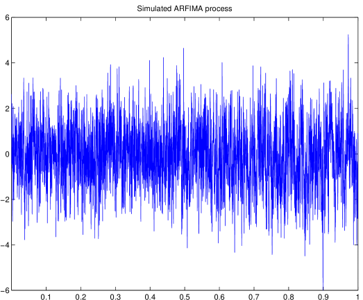
Figure 1. A simulated tvARFIMA(1,$d$,0) of length $T=2^{12}$.

We compute the local estimator $\widehat{\sigma}^{2}_{j,T}(u)$ defined in (23) with $\{\gamma_{j,T}(k)\}$ given by the kernel weights on the one hand and the recursive weights on the other hand, for $j=1,2,\dots,5$ with a bandwidth $\mathrm{b}_{T}=0.25$. For the kernel weight we took the rectangle kernel $K=\mathbbm{1}_{[-1/2,1/2]}$. The obtained local scalograms $\widehat{\sigma}^{2}_{j,T}(u)$ of the local wavelet spectrum $\sigma^{2}_{j}(u)$, $j=1,2,\dots,5$, $u\in[0,1]$ are represented in the lower parts of Figures 2 and 3, respectively, with a $y$-axis in a logarithmic scale.

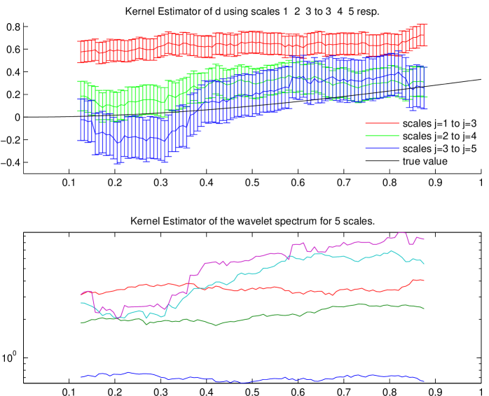
Figure 2. Local estimates as functions of $u\in[0,1]$ for the simulated tvARFIMA(1,$d$,0) using a two-sided rectangular kernel. Top: $\hat{d}_{T}(L;u)$ using scales $j=1,2,3$ to $3,4,5$ (respectively in blue, green and red) and the true value $d(u)$ (in thin black). Bottom: $\widehat{\sigma}^{2}_{j,T}(u)$ for $j=1,\dots,5$.

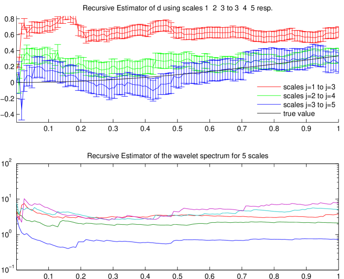
Figure 3. Same as Figure 2 using a recursive estimator.

The five corresponding curves exhibit different variabilities, the larger $j$, the larger the variability, which is in accordance with our theoretical findings. On the top of these two figures, we represented the true parameter $d(u)$, $u\in[0,1]$ (plain black) and the corresponding estimators $\widehat{d}_{T}(u)$ for three sets of scales, namely $j=1,2,3$ (blue line), $j=2,3,4$ (green line) and $j=3,4,5$ (red line), which correspond to $L=1,2,3$, respectively, and $\ell=2$ in the three sets of scales. The displayed bars centered at each estimate $\widehat{d}_{T}(u)$ represent 0.95 level confidence intervals, based on the asymptotic distribution given by (51). Since the asymptotic variance depends continuously on $d(u)$, we plug $\widehat{d}_{T}(u)$ in to compute each interval length. Numerical computations are done using the toolbox described in [13]. One can observe the difference between the two-side kernel estimator and the recursive estimator. The former exhibits a uniform behavior along time with border effects close to each boundaries of the interval $[0,1]$ (here we dropped the values of $\widehat{d}_{T}(u)$ for $u<\mathrm{b}_{T}/2$ and $u>1-\mathrm{b}_{T}/2$ to avoid these border effects). In contrast the latter exhibits a diminishing then stabilizing variability along time. Thus it is better adapted for estimating the right part of the interval. It is interesting to note that the choice of $L$ is crucial for this simulated example. This is due to the presence of an autoregressive component leading to a strong positive short-memory autocorrelation with a root close to the unit circle. As a result $d(u)$ is over estimated if a too low frequency band of scales is used (as in the case $L=1$), which explains why the true value mostly lies out of the corresponding confidence intervals. On the other hand this bias diminishes drastically as soon as $L\geq 2$, but, for $L=3$, the confidence intervals are larger since the normalizing term $\delta_{L,T}$ is larger. This larger variance is matched by the fact that the estimates are varying more widely for $L=3$. We made similar experiments for a tvARFIMA(0,$d$,0) process. In this case, this bias is no longer observed for $L=1$. We have also tried different values of the bandwidth $\mathrm{b}_{T}$ which also influences the bias and the variability of the estimates in the expected way. Finally we tested our procedures on longer series to check the numerical tractability. The computation of $\widehat{\sigma}^{2}_{j,T}(u)$ from $X_{1,T},\dots,X_{T,T}$, with $T=2^{15}$ took less than 1 second for the kernel estimator and 7 seconds for the recursive estimator with a 3.00GHz CPU. We note that the recursive version is about ten times slower than the kernel estimator. On the other hand the recursive estimator is adapted to online computation, that is, $\widehat{\sigma}^{2}_{j,T}(t)$ can be computed in a recursive fashion for each new available observation $X_{t,T}$.

5.2. Real data sets

We now use real data sets made of a sample of realized log volatility of the YEN versus USD exchange rate between June 1986 and September 2004. The realized log volatility is represented in Figure 4.

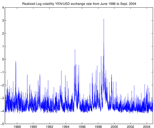
Figure 4. Realized log volatility of the YEN vs USD exchange rate from June 1986 to September 2004.

The series length is $T=4470$, that is of the same order as the previously simulated series ($T=2^{12}=4096$). Viewing the simulated data as a benchmark, we used approximately the same bandwidth parameter $\mathrm{b}_{T}=0.23$ and the same sets of scales, namely $L=1,2,3$ with $\ell=3$ in the three cases. The two-sided kernel estimators of the memory parameter are represented in the upper part of Figure 5. As previously we also display the corresponding local scalograms in the lower part of the same figure. We omit the results for the recursive estimator for brevity. One can observe that here as $L$ increases the estimates of $d(u)$ globally increases which may indicate a negative bias at high frequencies. We only plot the confidence intervals for the first 10 estimates for clarity. Indeed, in contrast to the simulated case, they largely cover each other, which indicates a less important bias. The green curve appears as a good compromise as in the simulated example. It exhibits a 5 years periodic-like behavior, which seems to indicate that the long memory parameter is not constant over time. This seems to be in accordance with the findings of [31] who model long-memory realized volatilities by a change of the model parameters from one regime to another where the different regimes can be explained by the influence of changing market factors (such as the Asian financial crisis of 1998).

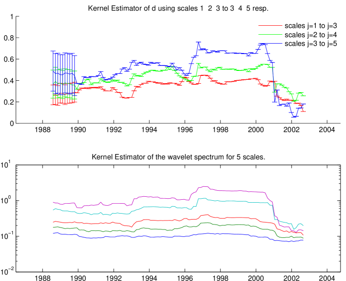
Figure 5. Same as Figure 2 for the YEN vs USD exchange rate realized log volatility.

6. Conclusion

In this paper we have delivered a semi-parametric, hence fairly general, approach for estimating the time-varying long-memory parameter $d(u)$ of a locally stationary process (or stationary increment process). Apart from modelling the singularity at zero frequency by the curve $d(u)$, we do not need to model the time varying spectrum of the remaining part explicitly. Using a wavelet log-regression estimator, already shown to be well-performing in the stationary situation, continues to work well due to a localization of the wavelet scalograms across time within each scale.

The development of our approach is based on a weakly stationary approximation at each given time point $u$. As in the stationary case, due to the generality of our semi-parametric spectral density not to be depending on only a finite number of parameters (as in [3], e.g.), we need to concentrate our attention to well estimating around frequency zero (where the amount of the long-memory effect measured by $d$ is visible). So a slightly subtle choice of considered scales for the log-regression has to be done: asymptotically we need that our estimator involves more and more frequencies (i.e. scales) but with a maximal frequency tending to zero. In the wavelet domain, this means that the lowest scale used in the estimator will be chosen so that i) the number of wavelet coefficients used in the estimator tends to infinity and ii) this lowest scale itself tends (slowly) to infinity.

Simulations have shown that our estimator performs reasonably well beyond being attractive from the point of view of asymptotic theory. In our real data analysis example, we adopt the approach of [31] and of [10] to assume that realized volatilities of some exchange rates follow a long-memory model. We make the interesting observation that for the observed series the long-memory parameter can clearly not be considered to be constant over time - which suggests that in explaining the persistent correlation in this exchange data there are certainly periods of stronger persistence followed by periods of weaker persistence.

Appendix A Postponed proofs

of Proposition 1.

By [23, Proposition 3], there is a constant $C_{1}$ such that, for all $j\geq 0$ and all $\lambda\in[-\pi,\pi]$,

$$|H_{j}(\lambda)|\leq C_{3}\,2^{j/2}\,|2^{j}\lambda|^{M}\,(1+2^{j}|\lambda|)^{-\alpha-M}\;.$$ (52)

Applying (1), (19), (15) and (20), we get, for any $u\in\mathbb{R}$, $j\geq 0$ and $k\in\{0,\dots,T_{j}-1\}$,

$$W_{j,k;T}=W_{j,k}(u)+R_{j,k}(u;T)\;,$$ (53)

where

$$R_{j,k}(u;T)=\int_{-\pi}^{\pi}\sum_{s\in\mathbb{Z}}\tilde{h}_{j,s}\left[A^{0}_{2^{j}k-s,T}(\lambda)-A(u;\lambda)\right]\mathrm{e}^{\mathrm{i}\lambda(2^{j}k-s)}\;\mathrm{d}Z(\lambda)\;.$$

The main approximation result consists in bounding

$$S_{j}(u;T)=\sum_{k=0}^{T_{j}-1}\gamma_{j,T}(k)R_{j,k}^{2}(u;T)$$

and

$$D_{j}(u;T)=\sum_{k=0}^{T_{j}-1}\gamma_{j,T}(k)W_{j,k}(u)R_{j,k}(u;T)\;.$$

In the following $C$ denotes some multiplicative constant. Using (3), (4), and (65) in Lemma 1, we have

$$\left|\sum_{s\in\mathbb{Z}}\tilde{h}_{j,s}\left[A^{0}_{2^{j}k-s,T}(\lambda)-A(u;\lambda)\right]\mathrm{e}^{\mathrm{i}\lambda(2^{j}k-s)}\right|\leq C\;2^{jp}\;|\lambda|^{-D}\;\left\{2^{j/2}\left|2^{j}k/T-u\right|+2^{3j/2}/T\right\}\;.$$

Recall that $D$ denotes an exponent less than $1/2$ which appears in the Conditions (3) and (4). Using $D<1/2$, we get

$$\mathbb{E}\left[R_{j,k}^{2}(u;T)\right]\leq C\;2^{2jp}\;2^{3j}\;T^{-2}\;\left\{1+(k-Tu2^{-j})^{2}\right\}\;.$$

Since we assumed $\alpha>1/2-d(u)$, we can take $D$ large enough so that $1-\alpha-d(u)<D<1/2$ (by adapting the constant $c$ appearing in the afore mentioned conditions). Hence we can assume in the following that

$$M>d(u)-1/2\quad\text{and}\quad d(u)+D+\alpha>1\;.$$ (54)

By (21) we also obtain that

$$\left|\mathbb{E}\left[W_{j,k}(u)R_{j,k}(u;T)\right]\right|\leq C\;2^{jp}\;\left\{2^{j/2}\left|2^{j}k/T-u\right|+2^{3j/2}/T\right\}\;\int_{-\pi}^{\pi}\left|\tilde{H}_{j}(\lambda)A(u;\lambda)\right|\;|\lambda|^{-D}\;\mathrm{d}\lambda$$

Using (18), (5), (6), $f^{*}(u,\lambda)\leq Cf^{*}(u,0)$ (by (7)), and (52), we further have

$$\int_{-\pi}^{\pi}\left|\tilde{H}_{j}(\lambda)A(u;\lambda)\right|\;|\lambda|^{-D}\;\mathrm{d}\lambda \leq C\;\int_{-\pi}^{\pi}\left|H_{j}(\lambda)\right|\ \sqrt{f(u,\lambda)}\;|\lambda|^{-D}\;\mathrm{d}\lambda$$

$$\leq C\;\sqrt{f^{*}(u,0)}\;2^{j(d(u)+D-1/2)}\;,$$

where we used that $\int_{\mathbb{R}}|\xi|^{M-d(u)-D}\ (1+|\xi|)^{-\alpha-M}\mathrm{d}(\xi)<\infty$ by (54). The last displays provide simple bounds for the expectations of $S_{j}$ and $D_{j}$.

To bound their variance, we use [27, Theorem 2, page 34], which yields

$$\mathrm{Cov}\left(R_{j,k}^{2}(u;T),R_{j,k^{\prime}}^{2}(u;T)\right)=2\mathrm{Cov}^{2}\left(R_{j,k}(u;T),R_{j,k^{\prime}}(u;T)\right)\\ +\mathrm{Cum}\left(R_{j,k}(u;T),R_{j,k}(u;T),R_{j,k^{\prime}}(u;T),R_{j,k^{\prime}}(u;T)\right)$$

and

$$\mathrm{Cov}\left(W_{j,k}(u)R_{j,k}(u;T),W_{j,k^{\prime}}(u)R_{j,k^{\prime}}(u;T)\right)\\ =\mathrm{Cov}\left(W_{j,k}(u),W_{j,k^{\prime}}(u)\right)\mathrm{Cov}\left(R_{j,k}(u;T),R_{j,k^{\prime}}(u;T)\right)\\ +\mathrm{Cov}\left(R_{j,k}(u;T),W_{j,k^{\prime}}(u)\right)\mathrm{Cov}\left(W_{j,k}(u),R_{j,k^{\prime}}(u;T)\right)\\ +\mathrm{Cum}\left(W_{j,k}(u),R_{j,k}(u;T),W_{j,k^{\prime}}(u),R_{j,k^{\prime}}(u;T)\right)\;.$$

Let us first provide bounds of $\mathbb{E}\left[R_{j,k}(u;T)R_{j,k^{\prime}}(u;T)\right]$ and $\mathbb{E}\left[W_{j,k}(u)R_{j,k^{\prime}}(u;T)\right]$ for $k,k^{\prime}=0,\dots,T_{j}-1$. Proceeding as previously, using (54), we get (in fact the cases above $k=k^{\prime}$ are particular cases)

$$\left|\mathbb{E}\left[R_{j,k}(u;T)R_{j,k^{\prime}}(u;T)\right]\right|\leq C\;2^{2jp}\;2^{3j}\;T^{-2}\;\left\{1+|k-Tu2^{-j}|\right\}\left\{1+|k^{\prime}-Tu2^{-j}|\right\}\;.$$

and

$$\left|\mathbb{E}\left[W_{j,k}(u)R_{j,k^{\prime}}(u;T)\right]\right|\leq C\;2^{jp}\;\sqrt{f^{*}(u;0)}\;2^{j(d(u)+D-1/2)}\;\left\{2^{j/2}\left|2^{j}k^{\prime}/T-u\right|+2^{3j/2}/T\right\}\;\;.$$

Using (10), we further get

$$\left|\mathrm{Cum}\left(R_{j,k}(u;T),R_{j,k}(u;T),R_{j,k^{\prime}}(u;T),R_{j,k^{\prime}}(u;T)\right)\right|\\ \leq C\;2^{4jp}\;2^{6j}\;T^{-4}\;\left\{1+(k-Tu2^{-j})^{2}\right\}\left\{1+(k^{\prime}-Tu2^{-j})^{2}\right\}\;,$$

and, denoting by $B_{j}(u)$ the variance of the (weakly stationary) process $\{W_{j,k}(u),\;k\in\mathbb{Z}\}$,

$$\left|\mathrm{Cum}\left(W_{j,k}(u),R_{j,k}(u;T),W_{j,k^{\prime}}(u),R_{j,k^{\prime}}(u;T)\right)\right|\\ \leq C\;B_{j}(u)\,2^{2jp}\;2^{3j}\;T^{-2}\;\left\{1+|k-Tu2^{-j}|\right\}\;\left\{1+|k^{\prime}-Tu2^{-j}|\right\}$$

Gathering these bounds, we obtain the same bound for $\mathrm{Var}^{1/2}\left(S_{j}(u;T)\right)$ and $\mathbb{E}\left[S_{j}(u;T)\right]$ and thus, using the definition of $\Gamma$ in (25),

$$\left|\mathbb{E}\left[S_{j}^{2}(u;T)\right]\right|^{1/2}\leq C\;2^{2jp}\;2^{3j}\;T^{-2}\;\{\Gamma_{0}(u;j,T)+\Gamma_{2}(u;j,T)\}\;.$$ (55)

For $D_{j}(u;T)$, we obtain

$$\left|\mathbb{E}\left[D_{j}(u;T)\right]\right|\leq C\;2^{jp}\;\sqrt{f^{*}(u;0)}\;2^{j(d(u)+D-1/2)}\;2^{3j/2}\;T^{-1}\;\{\Gamma_{0}(u;j,T)+\Gamma_{1}(u;j,T)\}\;.$$

We then obtain that $\mathrm{Var}^{1/2}\left(D_{j}(u;T)\right)$ is at most

$$C\;2^{jp}\;2^{3j/2}\;T^{-1}\;\{\Gamma_{0}(u;j,T)+\Gamma_{1}(u;j,T)\}\left\{B_{j}^{1/2}(u)+\sqrt{f^{*}(u;0)}\;2^{j(d(u)+D-1/2)}\right\}\;.$$

Observe that by [23, Theorem 1] we have, since $M>d(u)-1/2$ and $\alpha>1/2-d(u)$, $B_{j}(u)\leq C\;f^{*}(u;0)\;2^{2d(u)j}$. Hence, since $D<1/2$,

$$\left|\mathbb{E}\left[D_{j}^{2}(u;T)\right]\right|^{1/2}\leq C\;2^{jp}\;\sqrt{f^{*}(u;0)}\;2^{j(3/2+d(u))}\;T^{-1}\;\{\Gamma_{0}(u;j,T)+\Gamma_{1}(u;j,T)\}\;.$$ (56)

By (23) and (53), we have

$$\widehat{\sigma}^{2}_{j,T}(u)=\widetilde{\sigma}^{2}_{j,T}(u)+S_{j}(u;T)+D_{j}(u;T)\;,$$ (57)

where $\widetilde{\sigma}^{2}_{j,T}(u)$ is defined in (26). The bound (38) now follows from (55), (56), (57) and Assumption 2 (iv). ∎

of Theorem 1.

By (22) and (24),

$$\mathbb{E}\left[\widetilde{\sigma}^{2}_{j,T}(u)\right]=\mathbb{E}\left[W_{j,k}^{2}(u)\right]=\sigma^{2}_{j}(u)\;.$$ (58)

Since the wavelet coefficients (20) are those of a weakly stationary process, their behavior at large scales ($j\to\infty$) can be studied using [23, Theorem 1]. By [23, Theorem 1], since we assumed (7) and $M>d(u)-1/2$ and $\alpha>(1+\beta)/2-d(u)$, we obtain (40). In the following we denote

$$K^{*}_{u}=f^{*}(u,0)\mathbf{K}(d(u))\;.$$

We now provide a bound for

$$\mathrm{Var}\left(\widetilde{\sigma}^{2}_{j,T}(u)\right)=\sum_{k,k^{\prime}=0}^{T_{j}-1}\gamma_{j,T}(k)\gamma_{j,T}(k^{\prime})\mathrm{Cov}\left(W_{j,k}^{2}(u),W_{j,k^{\prime}}^{2}(u)\right)=V_{1}+V_{2}\;,$$

where the decomposition in $V_{1}+V_{2}$ follows from that of $\mathrm{Cov}\left(W_{j,k}^{2}(u),W_{j,k^{\prime}}^{2}(u)\right)$ in

$$2\mathrm{Cov}^{2}\left(W_{j,k}(u),W_{j,k^{\prime}}(u)\right)+\mathrm{Cum}\left(W_{j,k}(u),W_{j,k}(u),W_{j,k^{\prime}}(u),W_{j,k^{\prime}}(u)\right)\;.$$

We easily obtain that

$$V_{1}=2\int_{-\pi}^{\pi}\left|\Phi_{j,T}(\lambda;0,0)\right|^{2}\;\mathbf{D}_{j}^{\star 2}(\lambda)\;\mathrm{d}\lambda\;,$$ (59)

where $\mathbf{D}_{j}$ denotes the spectral density of the weakly stationary process $\{W_{j,k}\;,k\in\mathbb{Z}\}$, $\Phi_{j,T}$ is defined in (29) and, for any $(2\pi)$-periodic function $g$, $g^{\star 2}=g\star g(\lambda)=\int_{-\pi}^{\pi}g(\lambda-\xi)g(\xi)\mathrm{d}\xi$. Moreover, applying (8) with (21) and (29), we get that $V_{2}$ can be expressed as

$$\int_{[-\pi,\pi]^{4}}\prod_{k=1}^{4}\left[\tilde{H}_{j}(\lambda_{k})A(u;\lambda_{k})\right]\Phi_{j,T}(2^{j}(\lambda_{1}+\lambda_{2});0,0)\Phi_{j,T}(2^{j}(\lambda_{3}+\lambda_{4});0,0)\hat{\kappa}_{4}(\lambda)\;\mathrm{d}\mu(\lambda)\;.$$

Hence, bounding $\hat{\kappa}_{4}$, using (9) and setting $\lambda=\lambda_{1}+\lambda_{2}$, we have

$$|V_{2}|\leq c_{4}\int_{-\pi}^{\pi}\left|\aleph_{j}^{\star 2}(\lambda)\right|^{2}\;\left|\Phi_{j,T}(2^{j}\lambda;0,0)\right|^{2}\;\mathrm{d}\lambda\;,$$ (60)

where we set $\aleph_{j}(\lambda)=\tilde{H}_{j}(\lambda)\ A(u;\lambda)$. Observe that $\|\aleph_{j}^{\star 2}\|_{\infty}\leq\|\aleph_{j}\|_{2}^{2}=\|\mathbf{D}_{j}\|_{1}$ and $\|\mathbf{D}_{j}^{\star 2}\|_{\infty}\leq\|\mathbf{D}_{j}\|_{2}^{2}$. Now by [23, Theorem 1] we have, since $M\geq d(u)$ and $\alpha>1/2-d(u)$, $\|\mathbf{D}_{j}\|_{\infty}=O\left(2^{2jd(u)}\right)$ (the constants depend on $f^{*}(u;\cdot)$ only), which implies bounds of the same order for $\|\mathbf{D}_{j}\|_{1}$ and $\|\mathbf{D}_{j}\|_{2}$. Using (59), (60), Assumption 2(ii) with $i=i^{\prime}=v=v^{\prime}=0$ and observing that, by $(2\pi)$ periodicity of $|\Phi_{j,T}(\lambda;0,0)|$,

$$\int_{-\pi}^{\pi}\left|\Phi_{j,T}(2^{j}\lambda;0,0)\right|^{2}\;\mathrm{d}\lambda=\int_{-\pi}^{\pi}\left|\Phi_{j,T}(\lambda;0,0)\right|^{2}\;\mathrm{d}\lambda\;,$$

we finally get that

$$\mathrm{Var}\left(\widetilde{\sigma}^{2}_{j,T}(u)\right)=O(2^{4jd(u)}\delta_{j,T})\;.$$ (61)

Using (57) and (58), $\mathbb{E}\left[(\widehat{\sigma}^{2}_{j,T}(u)-K^{*}_{u}\;2^{2jd(u)})^{2}\right]$ is at most

$$C\;\left\{\mathrm{Var}\left(\widetilde{\sigma}^{2}_{j,T}(u)\right)+\mathbb{E}\left[S_{j}^{2}(u;T)\right]+\mathbb{E}\left[D_{j}^{2}(u;T)\right]\right\}+O\left(2^{2(2d(u)-\beta)j}\right)\\ =O\left(2^{4jd(u)}\delta_{j,T}+2^{(6+4p)j}T^{-4}\delta_{j,T}^{-4}+2^{(3+2p+2d(u))j}T^{-2}\delta_{j,T}^{-2}+2^{2(2d(u)-\beta)j}\right)\;.$$

where we used (61), (55), (56) and (33). Using (41), the last display gives (42). ∎

of Theorem 2.

Under the set of Assumptions (a), the proof immediately follows from [28, Theorem 2]. We now consider the set of Assumptions (b). In this case, we rely on the Gaussian assumption. The proof follows the lines of [21, Theorem 2], in which the stationary case is considered, i.e. $\gamma_{j,T}(u)=1$. We first observe that, for any $\mu=[\mu_{0}\,\,\dots\,\,\mu_{\ell}]^{T}\in\mathbb{R}^{\ell+1}$, we may write

$$\mu^{T}\widetilde{S}_{L}(u)=\xi_{L}^{T}\Delta_{L}\xi_{L}\;,$$

where $\xi_{L}$ is a Gaussian vector with entries $\left(W_{L+i,k}(u)\right)_{0\leq i\leq\ell,\,0\leq k\leq T_{L+i}}$ and $\Delta_{L}$ is the diagonal matrix with diagonal entries $\left(2^{-2Ld(u)}\delta_{L,T}^{-1/2}\mu_{i}\gamma_{L+i,T}(u)\right)_{0\leq i\leq\ell,\,0\leq k\leq T_{L+i}}$. We may thus apply [22, Lemma 12].

To obtain (43), it is thus sufficient to show that

$$\rho(\Delta_{L})\rho\left(\mathrm{Cov}(\xi_{L})\right)\to 0\;,$$ (62)

where $\rho(A)$ denotes the spectral radius of $A$, and

$$\mathrm{Cov}(\mu^{T}\widetilde{S}_{L}(u))\to(f^{*}(u,0))^{2}\mu^{T}\Sigma\mu\;.$$ (63)

We have, by (31) and Assumption 2(i),

$$\rho(\Delta_{L})\leq 2^{-2Ld(u)}\delta_{L,T}^{-1/2}\max_{0\leq i\leq\ell}|\mu_{i}|\max_{0\leq i\leq\ell}\delta_{L+i,T}=o\left(2^{-2Ld(u)}\right)\;.$$

Using [21, Lemma 6], [22, Lemma 11] and that $\mathbf{D}_{L+i}$ is the spectral density of the process $\{W_{L+i,k}(u),\,k\in\mathbb{Z}\}$, we have

$$\rho\left(\mathrm{Cov}(\xi_{L})\right)\leq\sum_{i=0}^{\ell}\rho\left(\mathrm{Cov}([W_{L+i,k}(u),\,k=0,\dots,T_{L+i}])\right)\leq 2\pi\sum_{i=0}^{\ell}\|\mathbf{D}_{L+i}\|_{\infty}\;.$$

By [23, Theorem 1], since we assumed $M\geq d(u)$ and $\alpha>1/2-d(u)$, we have $\|\mathbf{D}_{L+i}\|_{\infty}=O(2^{2Ld(u)})$. This with the last two displays implies (62).

We now compute the asymptotic covariance matrix of $\widetilde{S}_{L}(u)$. Let $0\leq j^{\prime}\leq j$. Using (30) and the Gaussian assumption, we have

$$\mathrm{Cov}\left(\widetilde{\sigma}^{2}_{j,T}(u),\widetilde{\sigma}^{2}_{j^{\prime},T}(u)\right) =\sum_{k=0}^{T_{j}-1}\sum_{k^{\prime}=0}^{T_{j^{\prime}}-1}\gamma_{j,T}(k)\gamma_{j^{\prime},T}(k^{\prime})\mathrm{Cov}\left(W_{j,k}^{2}(u),W_{j^{\prime},k^{\prime}}^{2}(u)\right)$$

$$=2\sum_{v=0}^{2^{j-j^{\prime}}-1}\sum_{k=0}^{T_{j}-1}\sum_{l\in\mathcal{T}_{j}(j-j^{\prime},v)}\gamma_{j,T}(k)\gamma_{j^{\prime},T}(l2^{j-j^{\prime}}+v)\mathrm{Cov}^{2}\left(W_{j,k}(u),W_{j^{\prime},l2^{j-j^{\prime}}+v}(u)\right)\;.$$

Using [23, Corollary 1], we have

$$\mathrm{Cov}\left(W_{j,k}(u),W_{j^{\prime},l2^{j-j^{\prime}}+v}(u)\right)=\int_{-\pi}^{\pi}\mathbf{D}_{j,j-j^{\prime},v}(\lambda)\mathrm{e}^{\mathrm{i}\lambda(k-l)}\,\mathrm{d}\lambda\;,$$

where $\mathbf{D}_{j,j-j^{\prime}}=[\mathbf{D}_{j,j-j^{\prime},v}]_{v=0,\dots,2^{j-j^{\prime}}-1}$ denotes the $2^{j-j^{\prime}}$-dimensional cross-spectral density between $W_{j,k}(u)$ and $[W_{j^{\prime},l2^{j-j^{\prime}}+v}(u)]_{v=0,\dots,2^{j-j^{\prime}}-1}$. It follows from the last two displays and (29) that

$$\mathrm{Cov}\left(\widetilde{\sigma}^{2}_{j,T}(u),\widetilde{\sigma}^{2}_{j^{\prime},T}(u)\right) =2\sum_{v=0}^{2^{j-j^{\prime}}-1}\int_{-\pi}^{\pi}\Phi_{j,T}(\lambda;0,0)\overline{\Phi}_{j,T}(\lambda;j-j^{\prime},v)\;\widetilde{\mathbf{D}}_{j,j-j^{\prime},v}(\lambda)\;\mathrm{d}\lambda\;,$$

where

$$\widetilde{\mathbf{D}}_{j,j-j^{\prime},v}(\lambda)=\int_{-\pi}^{\pi}\mathbf{D}_{j,j-j^{\prime},v}(\xi)\overline{\mathbf{D}}_{j,j-j^{\prime},v}(\xi-\lambda)\mathrm{d}\xi\;.$$

By [23, Theorem 1(b)], since we assumed $M\geq d(u)$ and $\alpha>1/2-d(u)$, using (7), we have, for $j=L+i$ and $j^{\prime}=L+i^{\prime}$ with $i^{\prime}\leq i$ fixed,

$$\|2^{-2d(u)j}\mathbf{D}_{j,j-j^{\prime}}-f^{*}(u,0)\mathbf{D}_{\infty,i-i^{\prime}}(\cdot;d(u))\|_{\infty}\to 0\;.$$

The last three displays, (45), Lemma 2 and Assumption 2 yield

$$\mathrm{Cov}\left(\widetilde{S}_{L,T}(u)\right)\to(f^{*}(u,0))^{2}\Sigma\;,$$

and hence (63). ∎

of Theorem 3.

We first show that

$$\delta_{L,T}^{-1/2}\left(\;2^{-2Ld(u)}\left[\begin{array}[]{c}\widehat{\sigma}^{2}_{L,T}(u)\\ \widehat{\sigma}^{2}_{L+1,T}(u)\\ \vdots\\ \widehat{\sigma}^{2}_{L+\ell,T}(u)\end{array}\right]-K^{*}_{u}\left[\begin{array}[]{c}1\\ 2^{2d(u)}\\ \vdots\\ 2^{2\ell d(u)}\end{array}\right]\right)\Rightarrow\mathcal{N}\left(0,(f^{*}(u,0))^{2}\Sigma(u)\right)\;.$$ (64)

Observe that the weak convergence (64) is the same as (47) except for the centering term. Relation (47) is valid since the assumptions of Corollary 1 hold. Applying $\delta_{L,T}\to 0$, Proposition 1 and the left-hand side condition of (50), we have that, for any $j=L+i$ with a fixed $i=0,\dots,\ell$,

$$\delta_{L,T}^{-1/2}2^{-2Ld(u)}\mathbb{E}\left[\widehat{\sigma}^{2}_{j,T}(u)\right]=\delta_{L,T}^{-1/2}2^{-2Ld(u)}\mathbb{E}\left[\widetilde{\sigma}^{2}_{j,T}(u)\right]+o(1)\;.$$

The bias control (40) and the right-hand side condition of (50) then imply

$$\delta_{L,T}^{-1/2}2^{-2Ld(u)}\mathbb{E}\left[\widehat{\sigma}^{2}_{j,T}(u)\right]=\delta_{L,T}^{-1/2}f^{*}(u,0)\mathbf{K}(d(u))2^{2id(u)}+o(1)\;.$$

This, with (47) gives the weak convergence (64) .

The convergence (51) now follows from (64) by applying the $\delta$-method as in [21, Proposition 3]. Indeed, define

$$g(x)=\sum_{i=0}^{\ell}w_{i}\log(x_{i})\quad\text{for all}\quad x=[x_{0}\,\,\dots\,\,x_{\ell}]^{T}\;.$$

Observe that, by (27) and (28), we have

$$g\left(2^{-2Ld(u)}[\widehat{\sigma}^{2}_{L,T}(u)\,\,\widehat{\sigma}^{2}_{L+1,T}(u)\,\,\dots\,\,\widehat{\sigma}^{2}_{L+\ell,T}(u)]^{T}\right)=\widehat{d}_{T}(L)$$

and

$$g\left(f^{*}(u,0)\mathbf{K}(d(u))[1\,\,2^{2d(u)}\,\,\dots\,\,2^{2\ell d(u)}]^{T}\right)=d(u)\;.$$

Thus (51) follows from (64) by computing the gradient of $g$ at the centering term,

$$\nabla g\left(f^{*}(u,0)\mathbf{K}(d(u))[1\,\,2^{2d(u)}\,\,\dots\,\,2^{2\ell d(u)}]^{T}\right)=\frac{[w_{0}\,\,w_{1}2^{-2d(u)}\,\,\dots\,\,w_{\ell}2^{-2\ell d(u)}]^{T}}{f^{*}(u,0)\mathbf{K}(d(u))}\;.$$

∎

Appendix B Technical lemmas

Lemma 1.

Assume (W-1)–(W-4). Let $h_{j,\cdot}$ the wavelet detail filter at scale index $j$ and $\tilde{h}_{j,\cdot}$ any factorization of it by $\mathbf{\Delta}^{p}$ with $p\in\{0,\dots,M\}$. Then we have

$$\sum_{s\in\mathbb{Z}}|\tilde{h}_{j,s}|\leq C\;2^{j(p+1/2)}\quad\text{and}\quad\sum_{s\in\mathbb{Z}}(1+|s|)\;|\tilde{h}_{j,s}|\leq C\;2^{j(p+3/2)}\;.$$ (65)

Lemma 2.

Suppose Assumption 2 holds. Let $i,i^{\prime}\geq 0$, $v\in\{0,\dots,2^{i}-1\}$ and $v^{\prime}\in\{0,\dots,2^{i^{\prime}}-1\}$. Define, for any $(2\pi)$-periodic function $g$,

$$I_{T}(g)=\delta_{j,T}^{-1}\int_{-\pi}^{\pi}\Phi_{j,T}(\lambda;i,v)\overline{\Phi_{j,T}(\lambda;i^{\prime},v^{\prime})}\;g(\lambda)\,\mathrm{d}\lambda\;.$$

Then the two following assertions hold.

1. If $h\to g$ in $L^{\infty}([-\pi,\pi])$, then $\displaystyle\sup_{T\geq 0}\left|I_{T}(h)-I_{T}(g)\right|\to 0$.

2. If $g\in L^{\infty}([-\pi,\pi])$ is continuous at zero, then, as $T\to\infty$, $\displaystyle I_{T}(g)\to V(i,v;i^{\prime},v^{\prime})\,g(0)$.

Proof.

By linearity of $I_{T}$, we may take $g=0$ to prove Assertion (i). We have, by the Cauchy-Schwarz inequality

$$\left|I_{T}(h)\right|\leq\|h\|_{\infty}\left[\delta_{j,T}^{-1/2}\|\Phi_{j,T}(\cdot;i,v)\|_{2}\right]\;\left[\delta_{j,T}^{-1/2}\|\Phi_{j,T}(\cdot;i^{\prime},v^{\prime})\|_{2}\right]\;.$$

Using Assumption 2(ii), the terms between brackets are bounded independently of $j$ and we obtain (i).

We now prove (ii). By linearity of $I_{T}$, we may assume $g(0)=1$. By Assumption 2(ii), we have $I_{T}(1)\to V(i,v;i^{\prime},v^{\prime})$. On the other hand, we have, for any $\eta>0$

$$\left|I_{T}(g)-I_{T}(1)\right| =\left|I_{T}((g-1)\mathbbm{1}_{[-\eta,\eta]}+(g-1)\mathbbm{1}_{[-\eta,\eta]^{c}})\right|$$

$$\leq\left|I_{T}((g-1)\mathbbm{1}_{[-\eta,\eta]})\right|+\left|I_{T}((g-1)\mathbbm{1}_{[-\eta,\eta]^{c}})\right|\;.$$

Observe that by continuity of $g$ at the origin, $\|(g-1)\mathbbm{1}_{[-\eta,\eta]}\|_{\infty}\to 0$ as $\eta\to\infty$. By (i), we get $\left|I_{T}((g-1)\mathbbm{1}_{[-\eta,\eta]})\right|\to 0$ as $\eta\to\infty$. It thus only remains to show that $\left|I_{T}((g-1)\mathbbm{1}_{[-\eta,\eta]^{c}})\right|\to 0$ for any $\eta>0$. This follows from the bound

$$\left|I_{T}((g-1)\mathbbm{1}_{[-\eta,\eta]^{c}})\right|\leq\|g-1\|_{1}\left[\delta_{j,T}^{-1/2}\sup_{\eta\leq|\lambda|\leq\pi}\left|\Phi_{j,T}(\lambda;i,v)\right|\right]\left[\delta_{j,T}^{-1/2}\sup_{\eta\leq|\lambda|\leq\pi}\left|\Phi_{j,T}(\lambda;i^{\prime},v^{\prime})\right|\right]\;,$$

and by applying Assumption 2(iii). ∎

Lemma 3.

For any $a>0$ and $b>0$, there exists $c>0$ such that

$$\left|z^{\alpha}-1\right|\leq c\,\{1+\log(|z|)\}\,\alpha\quad\text{for all}\quad\alpha\in[0,a],\,z\in\mathbb{C}\quad\text{with}\quad|z|\leq b\;.$$

Lemma 4.

Assume one of the following.

1. $K=\mathbbm{1}_{[-1/2,1/2]}$.

2. $K$ is compactly supported and $|\hat{K}(\xi)|=o(|\xi|^{-3/2})$ as $|\xi|\to\infty$, where $\hat{K}$ denotes the Fourier transform of $K$.

3. $K$ is integrable, $\hat{K}$ has an exponential decay, i.e. for some $c>0$, $|\hat{K}(\xi)|=O\left(\exp(-c|\xi|)\right)$ as $|\xi|\to\infty$, $K(t)=O(|t|^{-p_{0}})$ as $|t|\to\infty$ for some $p_{0}>3$, the derivative $K^{\prime}$ of $K$ satisfies $|K^{\prime}(t)|=O(|t|^{-p_{1}})$ as $|t|\to\infty$ for some $p_{1}>1$ and $T_{j}\exp(-c^{\prime}\mathrm{b}_{T}T_{j})=O(1)$ for any $c^{\prime}>0$.

Suppose that $\mathrm{b}_{T}\to 0$ and that $j$ depends on $T$ so that $T_{j}\mathrm{b}_{T}\to\infty$ as $T\to\infty$. Then, for weights given by (35), Assumption 2 is satisfied with

$$\delta_{j,T}\sim\frac{\|K\|_{\infty}}{\|K\|_{1}}(\mathrm{b}_{T}T_{j})^{-1}$$ (66)

$$V(i,v;i^{\prime},v^{\prime})=2\pi\,\frac{\|K\|_{2}^{2}}{\|K\|_{1}\|K\|_{\infty}}\;2^{-i-i^{\prime}}\,,\quad i,i^{\prime}\geq 0,\;0\leq v<2^{i},\,0\leq v^{\prime}<2^{i^{\prime}}\;.$$ (67)

Proof.

For convenience, we will omit the subscripts _T and _j,T in this proof section when no ambiguity arises. Under (K-1), one has $\rho=\mathrm{b}T_{j}+O(1)$. Under (K-2), $K$ is uniformly continuous on its compact support $S$ and, since $u\in(0,1)$, $\mathrm{b}\to 0$ and $T_{j}\mathrm{b}\to\infty$, $S$ eventually falls between the extremal points of $\{(uT_{j}-k)/(\mathrm{b}T_{j}),\,k=0,\dots,T_{j}-1\}$. Thus,

$$(\mathrm{b}T_{j})^{-1}\sum_{k=0}^{T_{j}-1}K((uT_{j}-k)/(\mathrm{b}T_{j}))\to\int_{S}K(s)\;\mathrm{d}s=\|K\|_{1}\;.$$

Under (K-3), using that $|K^{\prime}(t)|\leq c(1+|t|)^{-p_{1}}$ for some $p_{1}>1$ and $c>0$, we get

$$(\mathrm{b}T_{j})^{-1}\sum_{k=0}^{T_{j}-1}K((uT_{j}-k)/(\mathrm{b}T_{j}))-\int_{(u-1)/\mathrm{b}}^{u/\mathrm{b}}K(s)\;\mathrm{d}s =O\left((\mathrm{b}T_{j})^{-2}\sum_{l=0}^{T_{j}}(1+l/(\mathrm{b}T_{j}))^{-p_{1}}\right)$$

$$=O\left((\mathrm{b}T_{j})^{-1}\right)\;.$$

Hence the last three displays yield that, in all cases,

$$\rho_{j,T}\sim\|K\|_{1}(\mathrm{b}_{T}T_{j})\;.$$ (68)

The asymptotic equivalence (66) then follows from the definitions (35) and (31), and we obtain Assumption 2(i) by (16).

Let us now prove that Assumption 2(ii) holds under (K-1), (K-2) and (K-3), successively. Note that, by definition of (29), we have

$$\int_{-\pi}^{\pi}\Phi_{j,T}(\lambda;i,v)\overline{\Phi_{j,T}(\lambda;i^{\prime},v^{\prime})}\,\mathrm{d}\lambda=2\pi\sum_{l\in\mathcal{T}_{j}(i,v)\cap\mathcal{T}_{j}(i^{\prime},v^{\prime})}\gamma_{j-i,T}(2^{i}l+v)\gamma_{j-i^{\prime},T}(2^{i^{\prime}}l+v^{\prime})\;.$$ (69)

Under (K-1), using $2^{-i}T_{j-i}\sim 2^{-i^{\prime}}T_{j-i^{\prime}}\sim T_{j}$ by (31), $\mathrm{b}T_{j}\to\infty$ and $\mathrm{b}\to 0$, we easily get that the supports of the sequences $\{\gamma_{j-i,T}(2^{i}l+v),\,l\geq 0\}$ and $\{\gamma_{j-i^{\prime},T}(2^{i^{\prime}}l+v),\,l\geq 0\}$ are eventually included in $\mathcal{T}_{j}(i,v)\cap\mathcal{T}_{j}(i^{\prime},v^{\prime})$ and their intersection is of length asymptotically equivalent to $\mathrm{b}T_{j}$. Hence, using (69), (66) and (68) with $\|K\|_{1}=\|K\|_{\infty}=1$, we obtain that, in this case,

$$\delta^{-1}\int_{-\pi}^{\pi}\Phi_{j,T}(\lambda;i,v)\overline{\Phi_{j,T}(\lambda;i^{\prime},v^{\prime})}\,\mathrm{d}\lambda\sim 2\pi\,\frac{T_{j}^{2}}{T_{j-i}T_{j-i^{\prime}}}\;.$$

By (16), this is Assumption 2(ii) with $V(i,v;i^{\prime},v^{\prime})=2\pi 2^{-i-i^{\prime}}$ which coincides with (67) under (K-1).

Under (K-2), we proceed by interpreting the sum in (69) as a Riemann approximation of $\int K^{2}$ up to a normalization factor. For $l\in\mathcal{T}_{j}(i,v)\cap\mathcal{T}_{j}(i^{\prime},v^{\prime})$, we approximate

$$J_{l} =(\mathrm{b}T_{j})^{-1}\rho_{j-i,T}\rho_{j-i^{\prime},T}\gamma_{j-i,T}(2^{i}l+v)\gamma_{j-i^{\prime},T}(2^{i^{\prime}}l+v^{\prime})$$

$$=(\mathrm{b}T_{j})^{-1}\,K(\{uT_{j-i}-(2^{i}l+v)\}/\{\mathrm{b}T_{j-i}\})\,K(\{uT_{j-i^{\prime}}-(2^{i^{\prime}}l+v^{\prime})\}/\{\mathrm{b}T_{j-i^{\prime}}\})\;,$$

by the local average

$$\tilde{J}_{l}=\int_{I_{l}}K^{2}(s)\,\mathrm{d}s\;,$$

where $I_{l}$ is defined as the interval $[\{uT_{j}-(l+1)\}/\{\mathrm{b}T_{j}\},\{uT_{j}-l\}/\{\mathrm{b}T_{j}\}]$. Observe that

$$\sup_{s\in I_{l}}\left|s-\{uT_{j-i}-(2^{i}l+v)\}/\{\mathrm{b}T_{j-i}\}\right|\leq\frac{1}{\mathrm{b}T_{j}}+\left|\frac{1}{\mathrm{b}T_{j}}-\frac{2^{i}}{\mathrm{b}T_{j-i}}\right|\,|l-uT_{j}|+u\frac{|T_{j-i}-2^{i}T_{j}|}{\mathrm{b}T_{j-i}}\frac{|v|}{\mathrm{b}T_{j-i}}\;.$$

Using (16), $i,v=O(1)$ and $l=O(T_{j})$, we obtain, for any fixed integers $i$ and $v$,

$$\sup_{0\leq l\leq 2T_{j}}\sup_{s\in I_{l}}\left|s-\{uT_{j-i}-(2^{i}l+v)\}/\{\mathrm{b}T_{j-i}\}\right|=O((\mathrm{b}T_{j})^{-1})\;,$$ (70)

and the same holds if $i,v$ is replaced by $i^{\prime},v^{\prime}$. Note that

$$\mathcal{T}_{j}(i,v)\cap\mathcal{T}_{j}(i^{\prime},v^{\prime})=\{0,1\dots,\{2^{-i}(T_{j-i}-v)\}\wedge\{2^{-i^{\prime}}(T_{j-i^{\prime}}-v)\}-1\}\;,$$

which, by (16) and the fact that $K$ is compactly supported, is eventually contained in $\{0,1,\dots,2T_{j}\}$ and eventually contains the set of $l$’s such that $\tilde{J}_{l}\neq 0$, which is of size $O(\mathrm{b}T_{j})$. By (70), we also see that, out of a set of length $O(\mathrm{b}T_{j})$, both $J_{l}$ and $\tilde{J}_{l}$ vanish. Hence we have

$$\sum_{l\in\mathcal{T}_{j}(i,v)\cap\mathcal{T}_{j}(i^{\prime},v^{\prime})}\left|J_{l}-\tilde{J}_{l}\right|=O\left(\mathrm{b}T_{j}\sup_{l}|J_{l}-\tilde{J}_{l}|\right)\;.$$

Using (70) and the uniform continuity of $K$, there exists a constant $c$ such that

$$\sup_{l}|J_{l}-\tilde{J}_{l}|\leq(\mathrm{b}T_{j})^{-1}\sup_{|s-t|,|s-t^{\prime}|\leq c/(\mathrm{b}T_{j})}\left|K^{2}(s)-K(t)K(t^{\prime})\right|=o((\mathrm{b}T_{j})^{-1})\;.$$

The last two displays, (69) and the definitions of $J_{l}$ and $\tilde{J}_{l}$ thus yield

$$\frac{\rho_{j-i,T}\rho_{j-i^{\prime},T}}{\mathrm{b}T_{j}}\int_{-\pi}^{\pi}\Phi_{j,T}(\lambda;i,v)\overline{\Phi_{j,T}(\lambda;i^{\prime},v^{\prime})}\,\mathrm{d}\lambda\sim 2\pi\int K^{2}(s)\,\mathrm{d}s=2\pi\|K\|_{2}^{2}\;.$$ (71)

By (66) and (68), this gives Assumption 2(ii) with $V(i,v;i^{\prime},v^{\prime})$ given by (67).

Under (K-3), we proceed similarly but we can no longer use that $K$ has a compact support. Instead we use that $K$ is bounded and $|K^{\prime}(t)|\leq c^{\prime}(3+|t|)^{-p_{1}}$ for some $p_{1}>1$ and $c^{\prime}>0$ and thus, for any $c>0$, as soon as $(c+1)/(\mathrm{b}T_{j})\leq 1$,

$$\sup_{s\in I_{l}}\sup_{|t-s|,|t^{\prime}-s|\leq c/(\mathrm{b}T_{j})}\left|K^{2}(s)-K(t)K(t^{\prime})\right|\leq c^{\prime\prime}\,(\mathrm{b}T_{j})^{-1}(2+|uT_{j}-l|/(\mathrm{b}T_{j}))^{-p}\;.$$

With (70) and since the length of $\mathcal{T}_{j}(i,v)\cap\mathcal{T}_{j}(i^{\prime},v^{\prime})$ is $O(T_{j})$, we get

$$\sum_{l\in\mathcal{T}_{j}(i,v)\cap\mathcal{T}_{j}(i^{\prime},v^{\prime})}\left|J_{l}-\tilde{J}_{l}\right|=O\left((\mathrm{b}T_{j})^{-2}\sum_{k=0}^{T_{j}}(1+k/(\mathrm{b}T_{j}))^{-p}\right)=O\left((\mathrm{b}T_{j})^{-1}\right)\;.$$

Moreover

$$\sum_{l\in\mathcal{T}_{j}(i,v)\cap\mathcal{T}_{j}(i^{\prime},v^{\prime})}\tilde{J}_{l}=\int_{-u^{\prime}/\mathrm{b}}^{u/\mathrm{b}}K^{2}(s)\,\mathrm{d}s\to\|K\|_{2}^{2}\;,$$

where $u^{\prime}=[\{2^{-i}(T_{j-i}-v)\}\wedge\{2^{-i^{\prime}}(T_{j-i^{\prime}}-v^{\prime})\}]/T_{j}-u\to 1-u$ by (16). This yields (71) as in the previous case and thus the same conclusion holds.

Let us now show that Assumption 2 (iii) holds under (K-1), (K-2) and (K-3), successively. Under (K-1), we have

$$\left|\Phi(\lambda;i,v)\right|=\rho^{-1}_{j-i,T}\left|\sum_{k=1}^{N}\mathrm{e}^{\mathrm{i}k\lambda}\right|\;,$$

where $N=N_{j,T}$ denotes the number of $l\in\mathcal{T}_{j}(i,v)$ such that $\gamma_{j-i,T}(2^{i}l+v)>0$. Since the Dirichlet kernel satisfies

$$|D_{N}(\lambda)|=\left|\sum_{k=1}^{N}\mathrm{e}^{\mathrm{i}k\lambda}\right|=\left|\frac{\sin(\lambda N/2)}{\sin(\lambda/2)}\right|\;,$$

we observe that, for any $\eta>0$, $\sup_{N\geq 1}\sup_{\lambda\in[\eta,2\pi-\eta]}\left|D_{N}(\lambda)\right|<\infty$. Hence, with (66) and (68), we obtain Assumption 2 (iii).

Under (K-2) and (K-3), using that $K(t)=(2\pi)^{-1}\int\hat{K}(\xi)\,\mathrm{e}^{\mathrm{i}\xi t}\mathrm{d}\xi$, we get

$$\Phi(\lambda;i,v)=(2\pi\rho_{j-i,T})^{-1}\int_{-\infty}^{\infty}\;\hat{K}(\xi)\;\mathrm{e}^{\mathrm{i}\xi(uT_{j_{i}}-v)/(\mathrm{b}T_{j-i})}\;\sum_{l\in\tilde{\mathcal{T}}_{j}(i,v)}\mathrm{e}^{\mathrm{i}l(\lambda+2^{i}\xi/(\mathrm{b}T_{j-i}))}\,\mathrm{d}\xi\;,$$

where $\tilde{\mathcal{T}}_{j}(i,v)$ denotes the set of all $l\in\mathcal{T}_{j}(i,v)$ such that $\gamma_{j-i,T}(2^{i}l+v)$ does not vanish. Denote the length of $\tilde{\mathcal{T}}_{j}(i,v)$ by $N=N_{j,T}$ as in the previous case. We thus obtain

$$\left|\Phi(\lambda;i,v)\right|\leq(2\pi\rho_{j-i,T})^{-1}\int_{-\infty}^{\infty}\;\left|\hat{K}(\xi)\right|\;|D_{N}(\lambda+2^{i}\xi/(\mathrm{b}T_{j-i}))|\;\mathrm{d}\xi\;.$$

Let $\eta>0$. Splitting the above integral as $\int_{-\infty}^{\infty}=\int_{2^{i}|\xi|/(\mathrm{b}T_{j-i})\leq\eta/2}+\int_{2^{i}|\xi|/(\mathrm{b}T_{j-i})>\eta/2}$, we obtain

$$\sup_{\lambda\in[\eta,\pi]}\left|\Phi(\lambda;i,v)\right|\leq (2\pi\rho_{j-i,T})^{-1}\sup_{|\lambda|\in[\eta/2,\pi+\eta/2]}|D_{N}(\lambda)|$$

$$+(2\pi\rho_{j-i,T})^{-1}\|D_{N}\|_{\infty}\int_{2^{i}|\xi|/(\mathrm{b}T_{j-i})>\eta/2}\left|\hat{K}(\xi)\right|\mathrm{d}\xi\;.$$

Now, we have, for $\eta$ small enough, $\sup_{N\geq 1}\sup_{|\lambda|\in[\eta/2,\pi+\eta/2]}|D_{N}|(\lambda)<\infty$, $\|D_{N}\|_{\infty}\leq N$ and, under (K-2), $N=O(\mathrm{b}T_{j})$ and $\int_{2^{i}|\xi|/(\mathrm{b}T_{j-i})>\eta/2}\left|\hat{K}(\xi)\right|\mathrm{d}\xi=o((\mathrm{b}T_{j})^{-1/2})$, which, with the previous display, (66) and (68), implies Assumption 2 (iii). Under (K-3), the same conclusion holds using that $N=O(T_{j})$, $\int_{2^{i}|\xi|/(\mathrm{b}T_{j-i})>\eta/2}\left|\hat{K}(\xi)\right|\mathrm{d}\xi=O(\exp(-c2^{-i-1}\eta\mathrm{b}T_{j}))$ and $T_{j}\exp(-c^{\prime}\mathrm{b}T_{j-i})=O(1)$ with $c^{\prime}=c2^{-i-1}\eta$ .

Finally we show that Assumption 2 (iv) holds under (K-1), (K-2) and (K-3), successively. Using the definition (25) and (16), we get, for some positive constant $C$,

$$\Gamma_{q}(u;j,T)\leq C\frac{(\mathrm{b}T_{j})^{q}}{\rho_{j,T}}\sum_{k=0}^{T_{j}-1}K_{q}((uT_{j}-k)/(\mathrm{b}T_{j}))+O(\Gamma_{0}(u;j,T))\;,$$

where $K_{q}(x)=K(x)|x|^{q}$. By definition of $\rho_{j,T}$, one has $\Gamma_{0}(u;j,T)=O(1)$. Under (K-1) and (K-2), $K_{q}$ is bounded and compactly supported, so that $\sum_{k}K_{q}((uT_{j}-k)/(\mathrm{b}T_{j}))=O(\mathrm{b}T_{j})$. This, with (68) and the previous display, implies (33) for all $q\geq 0$. Hence, to conclude the proof, it only remains to show that, for $q=1,2$, under (K-3),

$$\sum_{k=0}^{T_{j}-1}K_{q}((uT_{j}-k)/(\mathrm{b}T_{j}))=O(\mathrm{b}T_{j})\;.$$

Using that $K(x)=O(|x|^{-p_{0}})$ as $x\to\pm\infty$, and $q\leq 2$, we separate the sum $\sum_{k=0}^{T_{j}-1}$ in $\sum_{|uT_{j}-k|\leq\mathrm{b}T_{j}}$ for which $K_{q}((uT_{j}-k)/(\mathrm{b}T_{j}))$ is $O(1)$ and $\sum_{|uT_{j}-k|>\mathrm{b}T_{j}}$ for which $K_{q}((uT_{j}-k)/(\mathrm{b}T_{j}))$ is $O(|(uT_{j}-k)/(\mathrm{b}T_{j})|^{2-p_{0}})$. Hence, we get

$$\sum_{k=0}^{T_{j}-1}K_{q}((uT_{j}-k)/(\mathrm{b}T_{j}))=O\left(\mathrm{b}T_{j}\right)+O\left(\mathrm{b}T_{j}^{p_{0}-2}\sum_{l\geq\mathrm{b}T_{j}-1}l^{2-p_{0}}\right)\;.$$

Observing that $\mathrm{b}T_{j}\to\infty$ and $p_{0}>3$, we obtain the desired bound. ∎

Lemma 5.

Suppose that $\mathrm{b}_{T}\to 0$ and $T_{j}\mathrm{b}_{T}\to\infty$. Then, for weights given by (37), Assumption 2 is satisfied with

$$\delta_{j,T}\sim(\mathrm{b}_{T}T_{j})^{-1}$$ (72)

$$V(i,v;i^{\prime},v^{\prime})=\pi\;2^{-i-i^{\prime}},\quad i,i^{\prime}\geq 0,\;v\in\{0,\dots,2^{i}-1\},\;v^{\prime}\in\{0,\dots,2^{i^{\prime}}-1\}\;.$$ (73)

Proof.

For convenience, we will omit the subscripts _T and _j,T in this proof when no ambiguity arises. We set $u_{j}=[u\,T_{j}]$ in the following. Using (36), $\mathrm{b}T_{j}\to\infty$, $\mathrm{b}\to 0$ and $u_{j}\sim uT_{j}$, we get that

$$\rho\sim(\mathrm{b}T_{j})\;.$$ (74)

Observing that $\delta=\gamma(u_{j})=\rho^{-1}$, we get (72) and Assumption 2(i) follows.

Let us now show that Assumption 2(ii) holds. Using (69), we find that

$$\int_{-\pi}^{\pi}\Phi_{j,T}(\lambda;i,v)\overline{\Phi_{j,T}(\lambda;i^{\prime},v^{\prime})}\,\mathrm{d}\lambda= \frac{2\pi}{\rho_{j-i,T}\rho_{j-i^{\prime},T}}\exp\left(-\frac{u_{j-i}+v+1}{\mathrm{b}T_{j-i}}-\frac{u_{j-i^{\prime}}+v^{\prime}+1}{\mathrm{b}T_{j-i^{\prime}}}\right)$$

$$\times\,\sum_{l=0}^{N-1}\mathrm{e}^{l\{2^{i}/(\mathrm{b}T_{j-i})+2^{i^{\prime}}/(\mathrm{b}T_{j-i^{\prime}})\}}\;,$$

where $N=\{2^{-i}(u_{j-i}-v)\}\wedge\{2^{-i^{\prime}}(u_{j-i^{\prime}}-v^{\prime})\}$. Using (16), (74), $\mathrm{b}T_{j}\to\infty$, $\mathrm{b}\to 0$ and $u_{j}\sim uT_{j}$, we obtain $\rho_{j-i,T}\sim 2^{i}(\mathrm{b}T_{j})$, $(u_{j-i}+v+1)/(\mathrm{b}T_{j-i})\sim u/\mathrm{b}$, $2^{i}/(\mathrm{b}T_{j-i})\sim 1/(\mathrm{b}T_{j})$, $N2^{i}/(\mathrm{b}T_{j-i})\sim u/\mathrm{b}$ and similar result with $i^{\prime},v^{\prime}$ replacing $i,v$. Using these asymptotic equivalences and the previous display, we obtain

$$\int_{-\pi}^{\pi}\Phi_{j,T}(\lambda;i,v)\overline{\Phi_{j,T}(\lambda;i^{\prime},v^{\prime})}\,\mathrm{d}\lambda\sim\frac{2\pi}{2^{i+i^{\prime}}(\mathrm{b}T_{j})^{2}}\frac{A-o(1)}{2/(\mathrm{b}T_{j})}\;,$$ (75)

where

$$A=\exp\left(-\frac{u_{j-i}+v+1}{\mathrm{b}T_{j-i}}-\frac{u_{j-i^{\prime}}+v^{\prime}+1}{\mathrm{b}T_{j-i^{\prime}}}+N\left\{\frac{2^{i}}{\mathrm{b}T_{j-i}}+\frac{2^{i^{\prime}}}{\mathrm{b}T_{j-i^{\prime}}}\right\}\right)\;.$$

Using (16), we have $N=uT_{j}+O(1)$ and $u_{j-i}+v+1=uT_{j}2^{i}+O(1)$. Thus $N2^{i}-(u_{j-i}+v+1)=O(1)$ and the same holds with $i^{\prime},v^{\prime}$ replacing $i,v$. This implies that $A=\exp\left(O\left((\mathrm{b}T_{j})^{-1}\right)\right)\to 1$. This, (75) and (72) yield Assumption 2(ii) with $V(i,v;i^{\prime},v^{\prime})$ defined by (73).

We finally show that Assumption 2(iii) holds. By setting $N=2^{-i}(u_{j-i}+v)$ and $k=N-1-l$ in (29), we obtain

$$\left|\Phi(\lambda;i,v)\right|=\rho^{-1}\left|\sum_{k=0}^{N-1}\mathrm{e}^{-k\{\mathrm{i}\lambda+2^{i}/(\mathrm{b}T_{j-i})\}}\right|\leq\rho^{-1}\frac{1+\mathrm{e}^{-N2^{i}/(\mathrm{b}T_{j-i})}}{\left|1-\mathrm{e}^{-\mathrm{i}\lambda-2^{i}/(\mathrm{b}T_{j-i})}\right|}\;.$$

Using that $N2^{i}/(\mathrm{b}T_{j-i})\sim\mathrm{b}^{-1}\to\infty$, $\delta^{-1/2}\rho^{-1}\to 0$ and that, for any $\eta>0$, $|1-z|$ does not vanish on the compact set of complex numbers $z=r\mathrm{e}^{\mathrm{i}\theta}$ such that $r\in[0,1]$ and $\eta\leq|\theta|\leq\pi$ and thus is lower bounded on this set, we obtain Assumption 2(iii).

Finally we show that Assumption 2 (iv) holds. By (16), we have, for any $q\geq 0$,

$$\Gamma_{q}(u;j,T)=\rho^{-1}\sum_{k=0}^{u_{j}-1}\mathrm{e}^{-(u_{j}-1-k)/(\mathrm{b}T_{j})}|u_{j}-1-k|^{q}+O\left(\Gamma_{0}(u;j,T)\right)\;.$$

Observe that $\Gamma_{0}(u;j,T)=1$. Setting $l=u_{j}-1-k$, and separating the above sum over $l\leq[q\mathrm{b}T_{j}]+1$ for which we bound the exponential by 1 and $l\geq[q\mathrm{b}T_{j}]+2$ so that $\mathrm{e}^{-x/(\mathrm{b}T_{j})}x^{q}$ is decreasing on $x\geq l-1$, we get

$$\sum_{k=0}^{u_{j}-1}\mathrm{e}^{-(u_{j}-1-k)/(\mathrm{b}T_{j})}|u_{j}-1-k|^{q} \leq\sum_{l=0}^{[\mathrm{b}T_{j}]+1}l^{q}+\sum_{l\geq[\mathrm{b}T_{j}]+2}\mathrm{e}^{-l/(\mathrm{b}T_{j})}l^{q}$$

$$\leq O\left((\mathrm{b}T_{j})^{q+1}\right)+\int_{x\geq[q\mathrm{b}T_{j}]+1}\mathrm{e}^{-x/(\mathrm{b}T_{j})}x^{q}\mathrm{d}x$$

$$=O\left((\mathrm{b}T_{j})^{q+1}\right)\;.$$

The last two displays, (74) and (72) yield (33), which achieves the proof. ∎

References

- Abry and Veitch [1998] Abry, P., Veitch, D., 1998. Wavelet analysis of long-range-dependent traffic. IEEE Trans. Inform. Theory 44 (1), 2–15.
-
Andersen et al. [2003]
Andersen, T. G., Bollerslev, T., Diebold, F. X., Labys, P., 2003. Modeling and
forecasting realized volatility. Econometrica 71 (2), 579–625.
URL http://dx.doi.org/10.1111/1468-0262.00418 -
Beran [2009]
Beran, J., 2009. On parameter estimation for locally stationary long-memory
processes. J. Statist. Plann. Inference 139 (3), 900–915.
URL http://dx.doi.org/10.1016/j.jspi.2008.05.047 - Dahlhaus [1996] Dahlhaus, R., 1996. On the Kullback-Leibler information divergence of locally stationary processes. Stochastic Process. Appl. 62 (1), 139–168.
- Dahlhaus [1997] Dahlhaus, R., 1997. Fitting time series models to non-stationary processes. Annals of Statistics 25, 1–37.
- Dahlhaus [2000] Dahlhaus, R., 2000. A likelihood approximation for locally stationary processes. Ann. Statist. 28 (6), 1762–1794.
-
Dahlhaus [2009]
Dahlhaus, R., 2009. Local inference for locally stationary time series based on
the empirical spectral measure. J. Econometrics 151 (2), 101–112.
URL http://dx.doi.org/10.1016/j.jeconom.2009.03.002 -
Dahlhaus and Neumann [2001]
Dahlhaus, R., Neumann, M., 2001. Locally adaptive fitting of semiparametric
models to nonstationary time series. Stochastic Process. Appl. 91 (2),
277–308.
URL http://dx.doi.org/10.1016/S0304-4149(00)00060-0 -
Dahlhaus and Subba Rao [2006]
Dahlhaus, R., Subba Rao, S., 2006. Statistical inference for time-varying
ARCH processes. Ann. Statist. 34 (3), 1075–1114.
URL http://dx.doi.org/10.1214/009053606000000227 - Ding et al. [1993a] Ding, Z., Engle, R., Granger, C., 1993a. A long memory property of stock market returns and a new model. Journal of Empirical Finance 1, 83–106.
-
Ding and Granger [1996]
Ding, Z., Granger, C. W. J., 1996. Modeling volatility persistence of
speculative returns: a new approach. J. Econometrics 73 (1), 185–215.
URL http://dx.doi.org/10.1016/0304-4076(95)01737-2 - Ding et al. [1993b] Ding, Z., Granger, C. W. J., Engle, R. F., 1993b. A long memory property of stock market returns and a new model. Journal of Empirical Finance 1 (1), 83–106.
- Faÿ et al. [2009] Faÿ, G., Moulines, E., Roueff, F., Taqqu, M., 2009. Estimators of long-memory: Fourier versus wavelets. J. of Econometrics (In press, DOI:10.1016/j.jeconom.2009.03.005).
- Faÿ et al. [2007] Faÿ, G., Roueff, F., Soulier, P., 2007. Estimation of the memory parameter of the infinite-source Poisson process. Bernoulli 13 (2), 473–491.
-
Fryzlewicz et al. [2008]
Fryzlewicz, P., Sapatinas, T., Subba Rao, S., 2008. Normalized least-squares
estimation in time-varying ARCH models. Ann. Statist. 36 (2), 742–786.
URL http://dx.doi.org/10.1214/07-AOS510 - Guégan and Lu [2009] Guégan, D., Lu, Z., 2009. Wavelet methods for locally stationary seasonal long memory processes, CES Working Paper 2009.15, Centre d’Economie de la Sorbonne.
-
Haldrup and Nielsen [2006]
Haldrup, N., Nielsen, M. Ø., 2006. A regime switching long memory model for
electricity prices. J. Econometrics 135 (1-2), 349–376.
URL http://dx.doi.org/10.1016/j.jeconom.2005.07.021 - Jensen and Whitcher [2000] Jensen, M. J., Whitcher, B., 2000. Time-varying long memory in volatility: Detection and estimation with wavelets, preprint, University of Missouri and Eurandom.
- Mikosch and Stărică [2004] Mikosch, T., Stărică, C., 2004. Changes of structure in financial time series and the Garch model. REVSTAT 2 (1), 41–73.
- Moulines et al. [2005] Moulines, E., Priouret, P., Roueff, F., 2005. On recursive estimation for time varying autoregressive processes. Ann. Statist. 33 (6), 2610–2654.
- Moulines et al. [2007a] Moulines, E., Roueff, F., Taqqu, M., 2007a. Central Limit Theorem for the log-regression wavelet estimation of the memory parameter in the Gaussian semi-parametric context. Fractals 15 (4), 301–313.
- Moulines et al. [2008] Moulines, E., Roueff, F., Taqqu, M., 2008. A wavelet Whittle estimator of the memory parameter of a non-stationary Gaussian time series. Ann. Statist. 36 (4), 1925–1956.
- Moulines et al. [2007b] Moulines, E., Roueff, F., Taqqu, M. S., 2007b. On the spectral density of the wavelet coefficients of long memory time series with application to the log-regression estimation of the memory parameter. J. Time Ser. Anal. 28 (2).
-
Ray and Tsay [2002]
Ray, B. K., Tsay, R. S., 2002. Bayesian methods for change-point detection in
long-range dependent processes. J. Time Ser. Anal. 23 (6), 687–705.
URL http://dx.doi.org/10.1111/1467-9892.00286 - Robinson [1995a] Robinson, P. M., 1995a. Gaussian semiparametric estimation of long range dependence. Ann. Statist. 23, 1630–1661.
- Robinson [1995b] Robinson, P. M., 1995b. Log-periodogram regression of time series with long range dependence. The Annals of Statistics 23, 1048–1072.
- Rosenblatt [1985] Rosenblatt, M., 1985. Stationary sequences and random fields. Birkhäuser Boston Inc., Boston, MA.
- Roueff and Taqqu [2009a] Roueff, F., Taqqu, M. S., 2009a. Asymptotic normality of wavelet estimators of the memory parameter for linear processes. J. Time Ser. Anal. 30 (5), 534–558.
- Roueff and Taqqu [2009b] Roueff, F., Taqqu, M. S., 2009b. Central limit theorems for arrays of decimated linear processes. Stoch. Proc. App. 119 (9), 3006–3041.
- Samorodnitsky [2006] Samorodnitsky, G., 2006. Long range dependence. Found. Trends Stoch. Syst. 1 (3), 163–257.
- Wang et al. [2008] Wang, S.-H., Hsiao, C., Bauwens, L., 2008. Forecasting long-memory processes subject to structural breaks, preprint, CORE, Université catholique de Louvain.
- Wornell and Oppenheim [1992] Wornell, G. W., Oppenheim, A. V., March 1992. Estimation of fractal signals from noisy measurements using wavelets. IEEE Trans. Signal Process. 40 (3), 611 – 623.