Collaborative Training in Sensor Networks:
A graphical model approach

Abstract

Graphical models have been widely applied in solving distributed inference problems in sensor networks. In this paper, the problem of coordinating a network of sensors to train a unique ensemble estimator under communication constraints is discussed. The information structure of graphical models with specific potential functions is employed, and this thus converts the collaborative training task into a problem of local training plus global inference. Two important classes of algorithms of graphical model inference, message-passing algorithm and sampling algorithm, are employed to tackle low-dimensional, parametrized and high-dimensional, non-parametrized problems respectively. The efficacy of this approach is demonstrated by concrete examples.

1 Introduction

It is widely recognized that distributed inference methods developed for graphical models comprise a principled approach for information fusion in sensor networks (see [1]). With powerful graphical model (GM) inference tools at hands, the similarity between sensor networks and graphical models compels researchers to model sensor network problems using graphical models so that the deeply researched GM algorithms, including sum-product, sampling and variational algorithms, can be applied to sensor networks.

Although this analogy seems to be simple, the map from sensor network problems to graphical models is not straightforward. As pointed out in [1], it is the informational structure of the distributed inference problem, involving the relationships between sensed information and the variables about which we wish to perform estimation, that is just as critical as the communication structure of the problem. How to model distributed inference problems as graphical models is as important as solving the problem itself. A wide range of distributed inference problems have been reformulated with graphical models, including self-localization [2], multi-object data association and tracking [3], [4], distributed hypothesis testing [5], and nonlinear distributed estimation [6].

One of the advantages of modeling distributed inference problems in sensor networks as inference problems on graphical models is to find communication-efficient “messages” that are exchanged among the sensors. In many ad-hoc algorithms for distributed inference problems, the messages transmitted among the sensors are problem-specific. If we can successfully model these problems as graphical models, the messages exchanged among the sensors turn out to be exactly the messages specified by the corresponding graphical model message-passing algorithms such as the sum-product algorithm.

Another issue, much more important in the area of wireless sensor networks than in graphical models, is the communication cost. In wireless sensor networks, communication is usually constrained and expensive, unlike in centralized inference algorithms, where message-passing is almost free. This difference leads to totally different optimization objectives in these two areas, even for exactly the same graphical models. In sensor network problems, we look for inference algorithms with more local computation and less message-passing; in graphical models, we are interested in algorithms that minimize the computational complexity. This brings us new problems like how to decrease the amount of data exchanged among the sensors, as described in [1], [7], [8], and [9]. This problem is unique for graphical models applied to distributed inference problems.

There are many distributed inference problems that have not been described in the language of graphical models. One type of such problem falls into the category of distributed learning/collaborative training, as described by Predd, et al., in [10], [11], and [12]. In these problems, the sensors collaboratively train their individual estimators so as to minimize the training error of a kernel regression, subject to consistency of prediction on shared data. In [11], an iterative algorithm is designed to achieve this training goal.

In our paper, we aim to model the distributed training problem as an inference problem on graphical models. In these settings, independent and identically distributed (i.i.d.) data are collected by different sensors, which are able to communicate with each other under some constrains. The sensors, without directly sharing their training data (usually high-dimensional, confidential and in large amount), attempt to collaboratively find a good ensemble classifier/estimator. In our framework, we manage to transform collaborative training problem, usually solved by an ad-hoc design (e.g. alternating projection) in a sensor network, into an inference problem on a graphical model combined with local training. This conversion from ad-hoc collaborative training to local training plus collaborative inference is due to the application of the graphical model on a functional space of classifiers/estimators. The problem of selecting the optimal estimator is converted into a maximum a posteriori probability (MAP) problem on a graphical model, with each random variable supported on a functional space to which the estimators belong.

2 From collaborative training to graphical models

The self-localization problem in [1] provides us with an excellent example of how to convert a distributed inference problem in a sensor network into an inference problem in a graphical model. Similar to this scheme, we design our graphical model for the collaborative training task to convert a “global collaborative training” into a “local training plus global inference” problem.

To make our model more concrete, we first illustrate the system in Fig. 1, where there are 6 sensors, with limited communication capability.

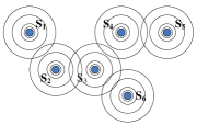
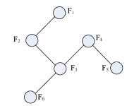
Fig. 1: A typical sensor network and its corresponding graphical model abstraction.

In Fig. 1, we abstract the sensor network into a graph. The edges among the nodes represent the condition that the nodes are able to communicate with each other. Now, we assume that each sensor $s$ maintains a distribution of estimators, i.e., a random variable $F_{s}$ supported by functional space $\mathcal{H}$, with probability distribution $\rho_{s}(f_{s})$.

Then, we assign a potential $\sigma_{s,t}(f_{s},f_{t})$ to the edge between two connected sensors $s$ and $t$. Here, $\sigma_{s,t}$ is a requirement of the similarity between the estimators maintained by adjacent sensors.

Based on these assumptions, the potential of the entire graphical model is of the form

$$p(f)=\frac{1}{Z}\prod_{s\in\mathcal{V}}\rho_{s}(f_{s})\prod_{(s,t)\in\mathcal{E}}\sigma_{s,t}(f_{s},f_{t}).$$ (1)

If the graph is loopless, a potential of the form (1) is a standard form to apply message-passing algorithms, such as the sum-product algorithm. These algorithms enable us to find the marginal distribution/MAP of the estimator at each sensor in a distributed way.

However, it is quite common that loops exist in the sensor network, yet it is very difficult to do triangulation in a system without centralized computation. To allow the use of message-passing algorithms, Willsky, et al. apply loopy belief propagation described in [13] and [14]. Although Jordan and Murphy in [14] have shown some cases where loopy belief propagation might lead to erroneous results, Willsky et al. have proven that under certain conditions, loopy belief propagation is a contractive map (for some specially defined distances) and hence converges to a unique limit. Therefore, loopy belief propagation can be applied to make inferences on the graphical model with potential (1). Moreover, sampling algorithms are not affected by loops, and can always be applied readily.

Under our framework, the messages or samples passed among the sensors are no longer data instances, but distributions or individual samples of functions. Thus, the sensors are no longer working with individual data points, but summaries of data - trained classifiers/estimators. Moreover, the message-passing algorithm ends in finite steps for loopless graphs, which requires no iteration. These advantages are due to the introduction of the graphical model.

3 Local Training and Global Inference

Based on the model described in the previous section, the problem now can be separated into two stages:

1. Local training: find reasonable potentials $\rho_{s}$ and $\sigma_{s,t}$;

2. Global inference: based on the potentials, compute the marginal distribution of estimators at each sensor.

We now discuss the details of these two stages.

3.1 Local Training for Potentials

There are two ways to obtain the potential $\rho_{s}$ based on local data. If there is a good model or prior knowledge of the parameters of $f_{s}$, then we can use local data to find $\rho_{s}$. However, in most of the cases, the distribution of parameters to be estimated is rather hard to compute explicitly. In this case, we can simply employ a bootstrap algorithm to re-sample the local training data for each individual sensor, and locally train a group of estimators, which can be used to approximate the distribution of the estimator. Thus, $\rho_{s}$ can be specified in a parametric (using the sample estimators to estimate the distribution of parameters) or non-parametric way (using several typical estimators as “particles”).

Finding $\sigma_{s,t}$ is more complicated. This is because in many cases, $\sigma_{s,t}$ is related to the statistical properties of the global estimator to be determined - i.e. it might be hard to estimate locally. In this paper, we restrict our discussion to problems where the entire system has one unique hypothesis. Thus, $\sigma_{s,t}$ is simply predetermined as

$$\sigma_{s,t}(f_{s},f_{t})=\left\{\begin{array}[]{ll}1&\mbox{$f_{s}$ and $f_{t}$ are the same}\\ 0&\mbox{otherwise}\end{array}\right.$$ (2)

although in practice, we sometimes need to relax the peaky function slightly. With the assumption above, we can discuss two classes of algorithms in graphical models for our collaborative training, message-passing (for parametrized, low-dimensional cases) and sampling (for non-parametrized, high-dimensionally cases).

Interestingly, it can be shown that for a simple hypothesis testing problem ($H_{0}$ vs. $H_{1}$), with the similarity function defined as in (2), the likelihood ratio methods (using the entire data set) and the collaborative training methods (computing the likelihood based on local data, and find marginal distribution by global inference) result in exactly the same outcome, given that the data collected by the sensors are i.i.d. To some extent, this supports the choice of our similarity function and the optimality of the scheme.

3.2 Message-Passing for Parametrized Cases

Message-passing is an accurate inference algorithm on graphical models. Here we assume that the classifier/estimator of sensor $s$ can be parametrized by parameter $x_{s}$.

Then, according to the sum-product algorithm described in [15], given the potential (1), the marginal at node $s$ is of the form

$$p(x_{s})\propto\rho(x_{s})\prod_{t\in\mathcal{N}(s)}M_{ts}^{*}(x_{s}),$$ (3)

where $M_{ts}^{*}(x_{s})$ is the message from sensor $t$ to sensor $s$. When the graph is loopless, the sum-product algorithm will converge in finitely many steps and converge to a unique limit. However, for arbitrary graph structure, the sum-product form might only be an approximation. Here we directly apply the message recursion update formula for the sum-product algorithm:

$$M_{ts}(x_{s})\leftarrow\sum_{x^{\prime}_{t}}\left\{\sigma_{s,t}(x_{s},x^{\prime}_{t})\rho(x^{\prime}_{t})\prod_{u\in\mathcal{N}(t)\backslash s}M_{ut}(x^{\prime}_{t})\right\}.$$ (4)

Specially, if we assume that the potentials are of Gaussian form,

$$\rho_{s}(x_{s})=\exp\left\{-\frac{(x_{s}-\mu_{s})^{2}}{2\sigma_{s}^{2}}\right\}$$ (5)

and

$$\sigma_{s,t}(x_{s},x_{t})=\exp\left\{-\frac{(x_{s}-x_{t})^{2}}{2\lambda_{s,t}^{2}}\right\},$$ (6)

where $\lambda_{s,t}$ is close to $0$ to ensure consensus, then the message is also of a Gaussian form:

$$M_{ts}(x_{s})=\exp\left\{-\frac{(x_{s}-\mu_{ts})}{2\sigma_{ts}^{2}}\right\}.$$ (7)

Therefore, message updating, as described in (4), can be simplified to an update of the parameters $\mu_{ts}$ and $\sigma_{ts}^{2}$, as specified below:

$$\mu_{ts}=\frac{\mu_{t}/\sigma_{t}^{2}+\sum_{u\in\mathcal{N}(t)\backslash s}\mu_{ut}/\sigma_{ut}^{2}}{1/\sigma_{t}^{2}+\sum_{u\in\mathcal{N}(t)\backslash s}1/\sigma_{ut}^{2}},$$ (8)

and

$$\sigma_{ts}^{2}=\lambda_{t,s}^{2}+\left(1/\sigma_{t}^{2}+\sum_{u\in\mathcal{N}(t)\backslash s}1/\sigma_{ut}^{2}\right)^{-1}.$$ (9)

After the messages converge, the marginal distribution $p_{s}(x_{s})$ of each sensor $s$ is still a Gaussian distribution with parameters given by

$$\hat{\mu}_{t}=\frac{\mu_{t}/\sigma_{t}^{2}+\sum_{u\in\mathcal{N}(t)}\mu_{ut}/\sigma_{ut}^{2}}{1/\sigma_{t}^{2}+\sum_{u\in\mathcal{N}(t)}1/\sigma_{ut}^{2}},$$ (10)

and

$$\hat{\sigma}_{t}^{2}=\left(1/\sigma_{t}^{2}+\sum_{u\in\mathcal{N}(t)}1/\sigma_{ut}^{2}\right)^{-1}.$$ (11)

It can be shown that when $\lambda_{s,t}\rightarrow 0$, and the network is loopless, the MAP estimation of each sensor after running message-passing converges to the average of $\mu_{s}$ weighted by $1/\sigma_{s}^{2}$, which is exactly how we combine i.i.d. Gaussian observations with different variances. In this sense, our scheme finds the optimal solution.

3.3 Sampling Algorithms for High-dimensional Cases

Message-passing for the parametrized case is straightforward. However, when the classifiers/estimators reside in some high-dimensional space (very common for most learning problems) and cannot easily be parametrized (like neural networks and decision trees), it is difficult to update the parameters directly and message-passing can be unimplementable. In this case, we resort to sampling methods to effectively search for the optimal classifiers/estimators.

The first problem we face is to find an expression for the distributions of estimators $f_{s}$ of individual sensors. Usually, by bootstrapping, we can obtain a group of “particles” $\{h_{sj}\}_{j=1}^{n_{s}}$ of the distribution of $f_{s}$. If we define a kernel $K(\cdot,\cdot)$ (non-negative), i.e. a measure of similarity of the estimators, then we can write the distribution of $f_{s}$ as

$$\rho_{s}(f_{s})=\sum_{j=1}^{n_{s}}K(h_{sj},f_{s}).$$ (12)

If we assume that the true hypothesis is unique, then we need to enforce consensus among the sensors; thus we define the similarity function as in (2).

With these assumptions, the marginal distribution of any sensor $t$ in (1) has the form (after summing out all the other variables)

$$p(f_{t})=\prod_{s=1}^{M}\sum_{j=1}^{n_{s}}K(h_{sj},f_{t}).$$ (13)

Therefore, the accurate MAP solution for the collaboratively trained estimator is given by

$$f^{*}=\operatorname*{arg\,max}_{f\in\mathcal{H}_{s}}\prod_{s=1}^{M}\sum_{j=1}^{n_{s}}K(h_{sj},f),$$ (14)

where $M$ represents the total number of sensors and $n_{s}$ is the number of “particles” bootstrapped by sensor $s$. Moreover, for simplicity, we define

$$\mathcal{H}_{s}=\left\{h_{sj}|s\in\{1,\ldots,M\},j\in\{1,\ldots,n_{s}\}\right\}.$$ (15)

It is difficult to apply an accurate inference algorithm to solve (14), because the closed-form messages involve an increasingly intricate product-sum of the kernels. Therefore, we resort to sampling methods to distributively tackle problem (14).

For simplicity, we only discuss the Gibbs Sampling case, which, in our model, reduces to the following algorithm:  
 

Repeat

1. Randomly select sensor $s$;

2. Fix the sample values of its neighbors $\{f_{t}\}_{t\in\mathcal{N}_{s}}$;

3. Conditioned on $\{f_{t}\}_{t\in\mathcal{N}_{s}}$, resample $f_{s}$ based on

the distribution of $f$

$\frac{1}{Z}\left(\prod_{t\in\mathcal{N}_{s}}\sigma_{s,t}(f_{t},f)\right)\left(\sum_{j=1}^{n_{s}}K(h_{sj},f)\right)$           where $f\in\{h_{sj}|1\leq j\leq n_{s}\}\cup\{f_{t}|t\in\mathcal{N}_{s}\}$;

End

Algorithm 1 Sampling Algorithm

In the algorithm, the function $\sigma_{s,t}(\cdot,\cdot)$ (non-negative) is the similarity function (a very peaky function). However, in practice, to make the sampling algorithm non-trivial and more forgiving, $\sigma_{s,t}$ should be relaxed, allowing some discrepancy between its two inputs, and thus preventing the algorithm from falling into a trivial solution. Moreover, notice that $\mathcal{N}_{s}$ represents the set of neighbors of sensor $s$, and the restrictions of the space in which $f$ resides is due to the locality constraints.

In practice, the algorithm might converge rather slowly. In that case, we can change the random resampling (step 3) of the algorithm into a deterministic optimization, i.e. we can replace step 3 by

$$f_{s}=\operatorname*{arg\,max}_{f\in\mathcal{H}_{s}}\left(\prod_{t\in\mathcal{N}_{s}}\sigma_{s,t}(f_{t},f)\right)\left(\sum_{j=1}^{n_{s}}K(h_{sj},f)\right).$$ (16)

This algorithm is prone to falling into a local minimum, yet converges faster. It is almost a greedy approach to finding the solution of (14).

There is one further subtle issue in implementing the sampling algorithm. Since the kernel is defined on various forms of classifiers/estimators, it might be hard sometimes, say, to define the similarity/distance between a decision tree and a neural network. If we define the prediction of estimator $f_{1}$ on the training set to be a vector $\mathbf{f}_{1}$ and the prediction of estimator $f_{2}$ on the training set to be a vector $\mathbf{f}_{2}$, then we use the similarity between these two vectors as that of the two estimators.

In the collaborative training scenario, however, the entire training set is not accessible to each individual sensor; thus $K$ and $\sigma_{s,t}$ can only be estimated locally, i.e., sensor $s$ can only compute $K$ and $\sigma_{s,t}$ based on its own data. Therefore, in the above algorithm, the kernels are actually subscripted. We will show empirically that this local data restriction indeed compromises the performance of the system, yet this is the price we pay for distributed algorithms.

The sampling algorithm has the advantage that only a properly selected kernel (a measure of similarity among classifiers) is required, unlike the case of message-passing, where we usually expect a linear Euclidean space of parameters. Moreover, sampling is not affected by the loops in the undirected graph model, and the sensors can update their samples asynchronously, as long as the samples of their Markov blankets are fixed.

4 Experiments

4.1 Message-Passing Algorithm: Linear Regression

Assume that $m$ sensors are distributed in the domain $[0,1]^{2}$. The sensors cooperate to estimate the slope $k$ of a straight line $z=kx$. The sensor at location $(x,y)\in[0,1]^{2}$ observes a noisy version of the value of $z$ at $x$, and the noise at point $(x,y)$ is additive and has a Gaussian distribution of variance $\sigma^{2}\sin^{2}(2\pi x)$. We also assume that each sensor can query the value of observations of its neighbors within a radius $r$.

For this problem, each sensor is capable of estimating the global model based on its own observation and those of its neighbors - because the slope $k$ can be estimated well even if we observe only a small part of the straight line. So for this consensus problem, the key step is to find the potential/distribution of each individual sensor. Bootstrapping is a suitable method in this case. Each sensor $s$ simply bootstraps over its accessible data (the data of itself and its neighbors) and uses the sample distribution to approximate the potential $\rho_{s}$. For computational simplicity, we parametrize these distributions as Gaussian (even though this is not accurate) so that we can simply apply the parameter update formula derived from the previous section.

There are 50 sensors with communication radius of 0.2 in this consensus problem, i.e. $m=50$, $r=0.2$ and $\lambda_{s,t}=0$. A typical result of the simulation is shown in Fig. 2.

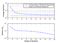
Fig. 2: Performance of the collaborative training algorithm running on the sensor network. The plot on top depicts the decreasing trend of the test error. The plot on the bottom demonstrates the attenuation of the variance of the estimated parameter, indicating the speed with which the system approaches consensus.

Note that the estimates of the slopes of different sensors in the distributed system come to consensus rather quickly - the variance of slopes among the sensors reduces to a negligible level after a few rounds. On the other hand, the average test error decreases quickly, very close to the performance of centralized linear regression.

4.2 Sampling Algorithm: Decision Tree Classifiers

We select the Chess data set (King-Rook vs. King-Pawn), a 3196-instance, 36-dimension, 2-class data set from the UCI machine learning repository, for this experiment. We randomly select 2000 data points, evenly distributed at 20 different sensors, as the training set, and use the remaining 1196 data points as the test set. The communication topology of the 20 sensors is a random graph of expected degree of 4. And each sensor, by bootstrapping, generates 4 classifiers (chosen to be standard decision tree classifiers provided by MATLAB). We define the kernel as

$$K(f_{s},f_{t})=\left(1-\frac{1}{n}\|\mathbf{f}_{s}-\mathbf{f}_{t}\|\right)^{4},$$ (17)

where $\mathbf{f}_{s}$ denotes the vector of prediction of classifier $f_{s}$ on all the local training data points, $\|\cdot\|$ denotes the Hamming distance of two 2-symbol vectors, and $n$ is the total number of local data. Moreover, we select $\sigma_{s,t}(\cdot,\cdot)$=$K(\cdot,\cdot)^{3}$ to make it a properly peaky function.

The sensors initialize their sampled classifiers by solving (14) based on their individual data (i.e., they solve the optimization problem of (14) without the product). Running the greedy version of the algorithm 1 for 4000 rounds, we obtain the results shown in Fig. 3 and Table 1.

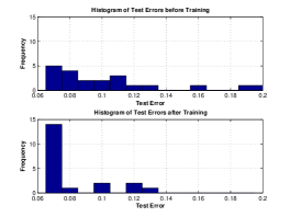
Fig. 3: Histograms of test errors among the sensors before and after running the sampling algorithm.

Data	Algorithm	Test Error
Centralized	Centralized decision tree	.0109
Distributed	Centralized solution to (14)	.0702
Distributed	Non-collaborative training	.0941 (median)
Distributed	Sampling algorithm	.0702 (median)
Distributed	Average of all classifiers	.0669

Table 1: Test errors of different algorithms, compared with the result of the sampling algorithm.

As shown in the results, the sampling algorithm (based on Gibbs Sampling) enables a major portion of the sensors in the network to find the optimal classifier, with respect to the distributed data, centralized solution to (14), and much better than the results given by non-collaborative training. A simple average of all the bootstrapped classifiers (similar to bagging) seems to be slightly better, yet the generated classifier is much more complicated than the results of the sampling algorithm (80 trees vs. 1 tree).

In this example, we have seen that our scheme of collaborative training can be quite effective even for a very complex, high-dimensional space of classifiers, without transmitting any training data points.

5 Conclusions and Discussions

We have applied our scheme to both parametrized, low-dimensional cases and non-parametrized, high-dimensional cases, and accurate message-passing and approximate sampling algorithms demonstrate their efficacy for these two cases separately. Without directly sharing data, the sensors are able to reach consensus and collaboratively search for a classifier/estimator satisfying certain optimality properties.

Although the “collaborative” part of our algorithms is based on message-passing or sampling algorithms borrowed from graphical models, another essential step of our algorithm is local training, as we only briefly resort to bootstrapping in this paper. It is of interest to find more detailed statistical tools to estimate these potentials, or more specifically, the distributions of classifiers/estimators so that we may be able to guarantee stronger optimality and obtain better performance.

Despite the issues and challenges described above, we have shown the efficacy of this framework with two different examples. It is worthwhile to design more delicate algorithms and to prove stronger results under this framework.

References

- [1] M. Cetin, L. Chen, J. W. Fisher III, A. T. Ihler, R. L. Moses, M. J. Wainwright, and A. S. Willsky, “Distributed fusion in sensor networks,” IEEE Signal Processing Magazine, vol. 23, no. 4, pp. 42–55, July 2006.
- [2] A. T. Ihler, J. W. Fisher III, R. L. Moses, and A. S. Willsky, “Nonparametric belief propagation for self-localization of sensor networks,” IEEE Journal on Selected Areas in Communications, vol. 23, no. 4, pp. 809–819, 2005.
- [3] L. Chen, M. J. Wainwright, M. Cetin, and A. S. Willsky, “Data association based on optimization in graphical models with application to sensor networks,” Mathematical and Computer Modelling, vol. 43, no. 9-10, pp. 1114–1135, 2006.
- [4] M. Uney and M. Cetin, “Graphical model-based approaches to target tracking in sensor networks: An overview of some recent work and challenges,” in Proc. 5th International Symposium on Image and Signal Processing and Analysis, Istanbul, Turkey, Sept. 2007, pp. 492–497.
- [5] R. Olfati-saber, E. Franco, E. Frazzoli, and J. S. Shamma, Belief Consensus and Distributed Hypothesis Testing in Sensor Networks, Springer, Berlin/Heidelberg, 2006.
- [6] C. Y Chong and S. Mori, “Graphical models for nonlinear distributed estimation,” in Proceedings of the 7th International Conference on Information Fusion, Stockholm, Sweden, July 2004, vol. 1, pp. 614–621.
- [7] O. P. Kreidl and A. Willsky, “Inference with minimal communication: A decision-theoretic variational approach,” in Advances in Neural Information Processing Systems 18, pp. 675–682. MIT Press, Cambridge, MA, 2006.
- [8] A. T. Ihler, Inference in Sensor Networks: Graphical Models and Particle Methods, Ph.D. thesis, Massachusetts Institute of Technology. Dept. of Electrical Engineering and Computer Science, Cambridge, MA, 2005.
- [9] E. B. Sudderth, A. T. Ihler, W. T. Freeman, and A. S. Willsky, “Nonparametric belief propagation,” in Proc. IEEE Computer Society Conference on Computer Vision and Pattern Recognition, Madison, WI, June 2003, vol. 1.
- [10] J. B. Predd, S. R. Kulkarni, and H. V. Poor, “A collaborative training algorithm for distributed learning,” IEEE Transactions on Information Theory, vol. 55, no. 4, pp. 1856–1871, April 2009.
- [11] J. B. Predd, S. R. Kulkarni, and H. V. Poor, “Distributed learning in wireless sensor networks,” IEEE Signal Processing Magazine, vol. 23, no. 4, pp. 56–69, July 2006.
- [12] J. B. Predd, S. R. Kulkarni, and H. V. Poor, “Distributed kernel regression: An algorithm for training collaboratively,” in Proc. IEEE Information Theory Workshop, Punta del Este, Uruguay, March 2006, pp. 332–336.
- [13] J. Pearl, Probabilistic Reasoning in Intelligent Systems: Networks of Plausible Inference, Morgan Kaufmann Publishers, San Mateo, CA, 1988.
- [14] K. P. Murphy, Y. Weiss, and M. I. Jordan, “Loopy belief propagation for approximate inference: An empirical study,” in Proceedings of Uncertainty in AI, Stockholm, Sweden, 1999, pp. 467–475.
- [15] M. J. Wainwright and M. I. Jordan, “A variational principle for graphical models,” in New Directions in Statistical Signal Processing. MIT Press, Cambridge, MA, 2005.