Global well-posedness for a nonlocal Gross-Pitaevskii equation with non-zero condition at infinity

Abstract

We study the Gross-Pitaevskii equation involving a nonlocal interaction potential. Our aim is to give sufficient conditions that cover a variety of nonlocal interactions such that the associated Cauchy problem is globally well-posed with non-zero boundary condition at infinity, in any dimension. We focus on even potentials that are positive definite or positive tempered distributions.

Keywords Nonlocal Schrödinger equation; Gross-Pitaevskii equation; Global well-posedness; Initial value problem.

Mathematics Subject Classification 35Q55; 35A05; 37K05; 35Q40; 81Q99.

1 Introduction

1.1 The problem

In order to describe the kinetic of a weakly interacting Bose gas of bosons of mass $m$, Gross [22] and Pitaevskii [33] derived in the Hartree approximation, that the wavefunction $\Psi$ governing the condensate satisfies

$$i\hbar\partial_{t}\Psi(x,t)=-\frac{\hbar^{2}}{2m}\Delta\Psi(x,t)+\Psi(x,t)\int_{\mathbb{R}^{N}}\lvert\Psi(y,t)\rvert^{2}V(x-y)\,dy,\text{ on $\mathbb{R}^{N}\times\mathbb{R},$}$$ (1)

where $N$ is the space dimension and $V$ describes the interaction between bosons. In the most typical first approximation, $V$ is considered as a Dirac delta function, which leads to the standard local Gross-Pitaevskii equation. This local model with non-vanishing condition at infinity has been intensively used, due to its application in various areas of physics, such as superfluidity, nonlinear optics and Bose-Einstein condensation [26, 25, 28, 11]. It seems then natural to analyze the equation (1) for more general interactions. Indeed, in the study of superfluidity, supersolids and Bose-Einstein condensation, different types of nonlocal potentials have been proposed [4, 13, 36, 34, 27, 1, 38, 12, 9].

To obtain a dimensionless equation, we take the average energy level per unit mass $\mathcal{E}_{0}$ of a boson, and we set

$$\psi(x,t)=\exp\left(\frac{im\mathcal{E}_{0}t}{\hbar}\right)\Psi(x,t).$$

Then (1) turns into

$$i\hbar\partial_{t}\psi(x,t)=-\frac{\hbar^{2}}{2m}\Delta\psi(x,t)-m\mathcal{E}_{0}\psi(x,t)+\psi(x,t)\int_{\mathbb{R}^{N}}\lvert\psi(y,t)\rvert^{2}V(x-y)\,dy.$$ (2)

Defining the rescaling

$$u(x,t)=\frac{1}{\lambda\sqrt{m\mathcal{E}_{0}}}\left(\frac{\hbar}{\sqrt{2m^{2}\mathcal{E}_{0}}}\right)^{\frac{N}{2}}\psi\left(\frac{\hbar x}{\sqrt{2m^{2}\mathcal{E}_{0}}},\frac{\hbar t}{m\mathcal{E}_{0}}\right),$$

from (2) we deduce that

$$i\partial_{t}u(x,t)+\Delta u(x,t)+u(x,t)\left(1-\lambda^{2}\int_{\mathbb{R}^{N}}\lvert u(y,t)\rvert^{2}\mathcal{V}(x-y)\,dy\right)=0,$$

with

$$\mathcal{V}(x)=V\left(\frac{\hbar x}{\sqrt{2m^{2}\mathcal{E}_{0}}}\right).$$

If we assume that the convolution between $\mathcal{V}$ and a constant is well-defined and equal to a positive constant, choosing $\lambda^{2}=(\mathcal{V}*1)^{-1},$ equation (2) is equivalent to

$$i{\partial}_{t}u+\Delta u+\lambda^{2}u(\mathcal{V}*(1-\lvert u\rvert^{2}))=0\textrm{ on }\mathbb{R}^{N}\times\mathbb{R}.\\$$ (3)

More generally, we consider the Cauchy problem for the nonlocal Gross-Pitaevskii equation with non-zero initial condition at infinity in the form

$$\left\{\begin{aligned} i{\partial}_{t}u+\Delta u+u(W*(1-\lvert u\rvert^{2}))&=0\textrm{ on }\mathbb{R}^{N}\times\mathbb{R},\\ u(0)&=u_{0},\end{aligned}\right.$$ (NGP)

where

$$\lvert u_{0}(x)\rvert\to 1,\quad\textrm{as}\quad\lvert x\rvert\to\infty.$$ (4)

If $W$ is a real-valued even distribution, (NGP) is a Hamiltonian equation whose energy given by

$$E(u(t))=\frac{1}{2}\int_{\mathbb{R}^{N}}\lvert\nabla u(t)\rvert^{2}\,dx+\frac{1}{4}\int_{\mathbb{R}^{N}}(W*(1-\lvert u(t)\rvert^{2}))(1-\lvert u(t)\rvert^{2})\,dx$$

is formally conserved.

In the case that $W$ is the Dirac delta function, (NGP) corresponds to the local Gross-Pitaevskii equation and the Cauchy problem in this instance has been studied by Béthuel and Saut [8], Gérard [19], Gallo [17], among others. As mentioned before, in a more general framework the interaction kernel $W$ could be nonlocal. For example, Shchesnovich and Kraenkel in [36] consider for $\varepsilon>0$,

$$W_{\varepsilon}({x})=\begin{cases}\dfrac{1}{2\pi\varepsilon^{2}\lvert x\rvert}K_{0}\left(\dfrac{\lvert x\rvert}{\varepsilon}\right),\quad N=2,\\ \dfrac{1}{4\pi\varepsilon^{2}\lvert x\rvert}\exp{\left(-\dfrac{\lvert x\rvert}{\varepsilon}\right)},\quad N=3,\end{cases}$$ (5)

where $K_{0}$ is the modified Bessel function of second kind (also called Macdonald function). In this way $W_{\varepsilon}$ might be considered as an approximation of the Dirac delta function, since $W_{\varepsilon}\to\delta$, as $\varepsilon\to 0,$ in a distributional sense. Others interesting nonlocal interactions are the soft core potential

$$W(x)=\begin{cases}1,&\ \text{ if }\lvert x\rvert<a,\\ 0,&\ \text{otherwise},\end{cases}$$ (6)

with $a>0$, which is used in [27, 1] to the study of supersolids, and also

$$W=\alpha_{1}\delta+\alpha_{2}K,\qquad\alpha_{1},\alpha_{2}\in\mathbb{R},$$ (7)

where $K$ is the singular kernel

$$K(x)=\dfrac{x_{1}^{2}+x_{2}^{2}-2x_{3}^{2}}{\lvert x\rvert^{5}},\quad x\in\mathbb{R}^{3}\backslash\{0\}.$$ (8)

The potential (7)-(8) models dipolar forces in a quantum gas (see [9], [38]).

1.2 Main results

In order to include interactions such as (7)-(8), it is appropriate to work in the space $\mathcal{M}_{p,q}(\mathbb{R}^{N})$, that is the set of tempered distributions $W$ such that the linear operator $f\mapsto W*f$ is bounded from $L^{p}(\mathbb{R}^{N})$ to $L^{q}(\mathbb{R}^{N})$. We denote by $\lVert W\rVert_{p,q}$ its norm. We will suppose that there exist

$$p_{1},p_{2},p_{3},p_{4},q_{1},q_{2},q_{3},q_{4},s_{1},s_{2}\in[1,\infty),$$

with

$$\frac{N}{N-2}>p_{4},\ \ \frac{2N}{N-2}>p_{2},p_{3},s_{1},s_{2}\geq 2,\ \ 2\geq q_{1}>\frac{2N}{N+2},\ \ q_{3},q_{4}>\frac{N}{2}\quad\text{ if }N\geq 3$$

and

$$p_{2},p_{3},s_{1},s_{2}\geq 2,\ \ 2\geq q_{1}>1\quad\text{ if }2\geq N\geq 1,$$

such that

$$\left\{\begin{aligned} &W\in\mathcal{M}_{2,2}(\mathbb{R}^{N})\cap\displaystyle\bigcap\limits_{i=1}^{4}\mathcal{M}_{p_{i},q_{i}}(\mathbb{R}^{N}),\\ &\dfrac{1}{p_{3}}+\dfrac{1}{q_{2}}=\dfrac{1}{q_{1}},\quad\dfrac{1}{p_{1}}-\dfrac{1}{p_{3}}=\dfrac{1}{s_{1}},\quad\dfrac{1}{q_{1}}-\dfrac{1}{q_{3}}=\dfrac{1}{s_{2}}\quad\text{ if }N\geq 3.\end{aligned}\right. \mathcal{W}_{N}$$ ()

We recall that if $p>q$, then $\mathcal{M}_{p,q}=\{0\}$. Therefore if we suppose that $W$ is not zero, the numbers above have to satisfy $q_{2},q_{3}\geq 2$. In addition, the existence of $s_{1}$, $s_{2}$ and the relations in (LABEL:Wn) imply that

$$\frac{N}{N-2}>p_{1},\ \ q_{2}>\frac{N}{2},\ \ \frac{1}{p_{1}}-\frac{1}{p_{3}}\in\left(\frac{N-2}{2N},\frac{1}{2}\right],\ \ \frac{1}{q_{1}}-\frac{1}{q_{3}}\in\left(\frac{N-2}{2N},\frac{1}{2}\right]\quad\text{ if }N\geq 3.$$

Figure 1 schematically shows the location of these numbers in the unit square.

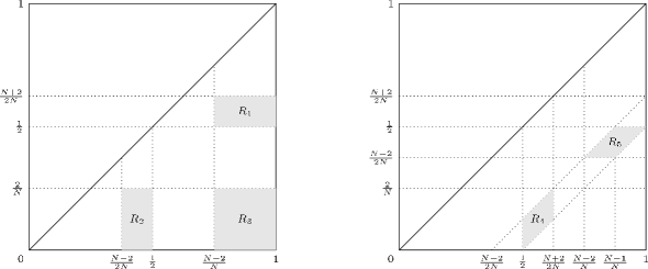
Figure 1: For $N>4$, the picture on the left represents the $(1/p,1/q)$-plane, in the sense that $(1/p_{1},1/q_{1})\in R_{1}$, $(1/p_{2},1/q_{2}),(1/p_{3},1/q_{3})\in R_{2}$, $(1/p_{4},1/q_{4})\in R_{3}$. In the picture on the right, the shaded areas symbolize that $(1/q_{1},1/q_{3})\in R_{4}$ and $(1/p_{1},1/p_{3})\in R_{5}$, for $N>6$.

To check the hypothesis (LABEL:Wn) it is convenient to use some properties of the spaces $\mathcal{M}_{p,q}(\mathbb{R}^{N})$. For instance, for any $1<p\leq q<\infty$, $\mathcal{M}_{p,q}(\mathbb{R}^{N})=\mathcal{M}_{q^{\prime},p^{\prime}}(\mathbb{R}^{N})$ and for any $1\leq p\leq 2$, $\mathcal{M}_{1,1}(\mathbb{R}^{N})\subseteq\mathcal{M}_{p,p}(\mathbb{R}^{N})\subseteq\mathcal{M}_{2,2}(\mathbb{R}^{N})$ ([20]). In Proposition 1.3 we give more explicit conditions to ensure (LABEL:Wn).

As remarked before, the energy is formally conserved if $W$ is a real-valued even distribution. We recall that a real-valued distribution is said to be even if

$$\langle W,\phi\rangle=\langle W,\widetilde{\phi}\rangle,\quad\forall\phi\in C_{0}^{\infty}(\mathbb{R}^{N};\mathbb{R}),$$

where $\widetilde{\phi}(x)=\phi(-x)$. However, the conservation of energy is not sufficient to study the long time behavior of the Cauchy problem, because the potential energy is not necessarily nonnegative and the nonlocal nature of the problem prevents us to obtain pointwise bounds. We are able to control this term assuming further that $W$ is a positive distribution or supposing that it is a positive definite distribution. More precisely, we say that $W$ is a positive distribution if

$$\langle W,\phi\rangle\geq 0,\quad\forall\phi\geq 0,\ \phi\in C_{0}^{\infty}(\mathbb{R}^{N};\mathbb{R}),$$

and that it is a positive definite distribution if

$$\langle W,\phi*\widetilde{\phi}\rangle\geq 0,\quad\phi\in C_{0}^{\infty}(\mathbb{R}^{N};\mathbb{R}).$$ (9)

These type of distributions frequently arise in the physical models (see Subsection 1.3). In particular, the real-valued even positive definite distributions include a large variety of models where the interaction between particles is symmetric. In Section 2 we state further properties of this kind of potentials.

As Gallo in [17], we consider the initial data $u_{0}$ for the problem (NGP) belonging to the space ${\phi}+H^{1}(\mathbb{R}^{N})$, with $\phi$ a function of finite energy. More precisely, from now on we assume that $\phi$ is a complex-valued function that satisfies

$$\phi\in W^{1,\infty}(\mathbb{R}^{N}),\ \nabla\phi\in H^{2}(\mathbb{R}^{N})\cap C(B^{c}),\ \lvert\phi\rvert^{2}-1\in L^{2}(\mathbb{R}^{N}),$$ (10)

where $B^{c}$ denotes the complement of some ball $B\subseteq\mathbb{R}^{N}$, so that in particular $\phi$ satisfies (4).

Remark 1.1.

We do not suppose that $\phi$ has a limit at infinity. In dimensions $N=1,2$ a function satisfying (10) could have complicated oscillations, such as (see [19, 18])

$$\phi(x)=\exp(i(\ln(2+\lvert x\rvert))^{\frac{1}{4}}),\quad x\in\mathbb{R}^{2}.$$

We note that any function verifying (10) belongs to the Homogeneous Sobolev space

$$\dot{H}^{1}(\mathbb{R}^{N})=\{\psi\in L^{2}_{\operatorname{loc}}(\mathbb{R}^{N}):\nabla\psi\in L^{2}(\mathbb{R}^{N})\}.$$

In particular, if $N\geq 3$ there exists $z_{0}\in\mathbb{C}$ with $\lvert z_{0}\rvert=1$ such that $\phi-z_{0}\in L^{\frac{2N}{N-2}}(\mathbb{R}^{N})$ (see e.g. Theorem 4.5.9 in [24]). Choosing $\alpha\in\mathbb{R}$ such that $z_{0}=e^{i\alpha}$ and since the equation (NGP) is invariant by a phase change, one can assume that $\phi-1\in L^{\frac{2N}{N-2}}(\mathbb{R}^{N})$, but we do not use explicitly this decay in order to handle at the same time the two-dimensional case.

Our main result concerning the global well-posedness for the Cauchy problem is the following.

Theorem 1.2.

Let $W$ be a real-valued even distribution satisfying (LABEL:Wn).

• Assume that one of the following is verified

  • $N\geq 2$ and $W$ is a positive definite distribution.

  • $N\geq 1$, $W\in\mathcal{M}_{1,1}(\mathbb{R}^{N})$ and $W$ is a positive distribution.

  Then the Cauchy problem (NGP) is globally well-posed in $\phi+H^{1}(\mathbb{R}^{N})$. More precisely, for every $w_{0}\in H^{1}(\mathbb{R}^{N})$ there exists a unique $w\in C(\mathbb{R},H^{1}(\mathbb{R}^{N}))$, for which $\phi+w$ solves (NGP) with the initial condition $u_{0}=\phi+w_{0}$ and for any bounded closed interval $I\subset\mathbb{R}$, the flow map $w_{0}\in H^{1}(\mathbb{R}^{N})\mapsto w\in C(I,H^{1}(\mathbb{R}^{N}))$ is continuous. Furthermore, $w\in C^{1}(\mathbb{R},H^{-1}(\mathbb{R}^{N}))$ and the energy is conserved

  $$E_{0}:=E(\phi+w_{0})=E(\phi+w(t)),\ \forall t\in\mathbb{R}.$$ (11)

• Assume that there exists $\sigma>0$ such that

  $$\operatorname*{ess\,inf}\widehat{W}\geq\sigma.$$ (12)

  Then (NGP) is globally well-posed in $\phi+H^{1}(\mathbb{R}^{N})$, for all $N\geq 1$ and (11) holds. Moreover, if $u$ is the solution associated to the initial data $u_{0}\in\phi+H^{1}(\mathbb{R}^{N})$, we have the growth estimate

  $$\lVert u(t)-\phi\rVert_{L^{2}}\leq C\lvert t\rvert+\lVert u_{0}-\phi\rVert_{L^{2}},$$ (13)

  for any $t\in\mathbb{R}$, where $C$ is a positive constant that depends only on $E_{0}$, $W,$ $\phi$ and $\sigma$.

We make now some remarks about Theorem 1.2.

• The condition (LABEL:Wn) implies that $W\in\mathcal{M}_{2,2}(\mathbb{R}^{N})$, so that $\widehat{W}\in L^{\infty}(\mathbb{R}^{N})$ and therefore the condition (12) makes sense.

• In contrast with (13), as we prove in Section 5, the growth estimate for the solution given by Theorem 1.2-(i) is only exponential

  $$\lVert u(t)-\phi\rVert_{L^{2}}\leq C_{1}e^{C_{2}\lvert t\rvert}(1+\lVert u_{0}-\phi\rVert_{L^{2}}),\qquad t\in\mathbb{R},$$

  for some constants $C_{1},C_{2}$ only depending on $E_{0}$, $W$ and $\phi$.

• Accordingly to Remark 1.1 and the Sobolev embedding theorem, after a phase change independent of $t$, the solution $u$ of (NGP) given by Theorem 1.2 also satisfies that $u-1\in L^{\frac{2N}{N-2}}(\mathbb{R}^{N})$ if $N\geq 3$.

• In dimensions $1\leq N\leq 3$ we can choose $(p_{4},q_{4})=(2,2)$ in (LABEL:Wn). Consequently, the condition that $W\in\mathcal{M}_{p_{4},q_{4}}(\mathbb{R}^{N})$ is nontrivial only when $N\geq 4$.

At first sight, it is not obvious to check the hypotheses on $W$. The purpose of the next result is to give sufficient conditions to ensure (LABEL:Wn).

Proposition 1.3.

• Let $1\leq N\leq 3$. If $W\in\mathcal{M}_{2,2}(\mathbb{R}^{N})\cap\mathcal{M}_{3,3}(\mathbb{R}^{N})$, then $W$ fulfils (LABEL:Wn). Furthermore, if $W$ verifies (LABEL:Wn) with $p_{i}=q_{i}$, $1\leq i\leq{3}$, then $W\in\mathcal{M}_{2,2}(\mathbb{R}^{N})\cap\mathcal{M}_{3,3}(\mathbb{R}^{N})$.

• Let $N\geq 4$. Assume that $W\in\mathcal{M}_{r,r}(\mathbb{R}^{N})$ for every $1<r<\infty$. Also suppose that there exists $\bar{r}>\frac{N}{4}$ such that $W\in\mathcal{M}_{p,q}(\mathbb{R}^{N})$, for every $1-\frac{1}{\bar{r}}<\frac{1}{p}<1$ with $\frac{1}{q}=\frac{1}{p}+\frac{1}{\bar{r}}-1$. Then $W$ satisfies (LABEL:Wn).

We conclude from Proposition 1.3 that the Dirac delta function verifies (LABEL:Wn) in dimensions $1\leq N\leq 3$. Since $\widehat{\delta}=1$, Theorem 1.2-(ii) recovers the results of global existence for the local Gross-Pitaevskii equation in [8, 19, 17] and the growth estimate proved in [2]. In addition, if the potential converges to the Dirac delta function, the correspondent solutions converge to the solution of the local problem as a consequence of the following result.

Proposition 1.4.

Assume that $1\leq N\leq 3$. Let $(W_{n})_{n\in\mathbb{N}}$ be a sequence of real-valued distributions in $\mathcal{M}_{2,2}(\mathbb{R}^{N})\cap\mathcal{M}_{3,3}(\mathbb{R}^{N})$ such that $u_{n}$ is the global solution of (NGP) given by Theorem 1.2, with $W_{n}$ instead of $W,$ for some initial data in $\phi+H^{1}(\mathbb{R}^{N})$, and

$$\lim_{n\to\infty}W_{n}={W_{\infty}},\quad\textup{ in }\ \mathcal{M}_{2,2}(\mathbb{R}^{N})\cap\mathcal{M}_{3,3}(\mathbb{R}^{N}),$$ (14)

with $\lVert W_{\infty}\rVert_{\mathcal{M}_{2,2}\cap\mathcal{M}_{3,3}}>0$ ($\lVert\cdot\rVert_{\mathcal{M}_{2,2}\cap\mathcal{M}_{3,3}}:=\max\{\lVert\cdot\rVert_{\mathcal{M}_{2,2}},\lVert\cdot\rVert_{\mathcal{M}_{3,3}}\}$). Then $u_{n}\to u$ in $C(I,H^{1}(\mathbb{R}^{N}))$, for any bounded closed interval $I\subset\mathbb{R}$, where $u$ is the solution of (NGP) with $W={W_{\infty}}$ and the same initial data.

On the other hand, the Dirac delta function does not satisfy (LABEL:Wn) if $N\geq 4$ and therefore Theorem 1.2 cannot be applied. In fact, to our knowledge there is no proof for the global well-posedness to the local Gross-Pitaevskii equation in dimension $N\geq 4$ with arbitrary initial condition. For small initial data, Gustafson et al. [23] proved global well-posedness in dimensions $N\geq 4$ as well as Gérard [19] in the four-dimensional energy space.

As a consequence of Theorem 1.2 and Proposition 1.3 we derive the next result for integrable kernels.

Corollary 1.5.

Let $W$ be a real-valued even function such that $W\in L^{1}(\mathbb{R}^{N})$ if $1\leq N\leq 3$ and $W\in L^{1}(\mathbb{R}^{N})\cap L^{r}(\mathbb{R}^{N})$, for some $r>\frac{N}{4}$, if $N\geq 4$. Assume also that $W$ is positive definite if $N\geq 2$, or that it is nonnegative. Then the Cauchy problem (NGP) is globally well-posed in $\phi+H^{1}(\mathbb{R}^{N})$.

As Gallo remarks in [17], the well-posedness in a space such as $\phi+H^{1}(\mathbb{R}^{N})$ makes possible to handle the problem with initial data in the energy space

$$\mathcal{E}(\mathbb{R}^{N})=\{u\in H^{1}_{\textrm{loc}}(\mathbb{R}^{N}):\nabla u\in L^{2}(\mathbb{R}^{N}),\ 1-\lvert u\rvert^{2}\in L^{2}(\mathbb{R}^{N})\},$$

equipped with the distance

$${d}(u,v)=\lVert u-v\rVert_{X^{1}+H^{1}}+\lVert\lvert u\rvert^{2}-\lvert v\rvert^{2}\rVert_{L^{2}}.$$ (15)

Here $X^{1}(\mathbb{R}^{N})$ denotes the Zhidkov space

$$X^{1}(\mathbb{R}^{N})=\{u\in L^{\infty}(\mathbb{R}^{N}):\nabla u\in L^{2}(\mathbb{R}^{N})\}.$$

We recall that $u\in C(\mathbb{R},\mathcal{E}(\mathbb{R}^{N}))$ is called a mild solution of (NGP) if it satisfies the Duhamel formula

$${u(t)=e^{it\Delta}u_{0}+i\int_{0}^{t}e^{i(t-s)\Delta}(u(s)(W*(1-\lvert u(s)\rvert^{2}))\,ds,\quad t\in\mathbb{R}.}$$

We note that by Lemma 6.3 the integral in the r.h.s is actually finite (see [19, 18] for further results about the action of Schrödinger semigroup on $\mathcal{E}(\mathbb{R}^{N})$). With the same arguments of [17], we may also handle the problem with initial data in the energy space. Moreover, in the case $1\leq N\leq 4$, we prove that a solution in the energy space with initial condition $u_{0}\in\mathcal{E}(\mathbb{R}^{N})$, necessarily belongs to $u_{0}+H^{1}(\mathbb{R}^{N})$, which is a proper subset of $\mathcal{E}(\mathbb{R}^{N})$. This also gives the uniqueness in the energy space for $1\leq N\leq 4$, as follows.

Theorem 1.6.

Let $W$ be as in Theorem 1.2. Then for any $u_{0}\in\mathcal{E}(\mathbb{R}^{N})$, there exists a unique $w\in C(\mathbb{R},H^{1}(\mathbb{R}^{N}))$ such that $u:=u_{0}+w$ solves (NGP). Furthermore, if $1\leq N\leq 4$ and $v\in C(\mathbb{R},\mathcal{E}(\mathbb{R}^{N}))$ is a mild solution of (NGP) with $v(0)=u_{0}$, then $v=u$.

The next proposition shows that the hypotheses made on the potential $W$ also ensure the $H^{2}$-regularity of the solutions.

Proposition 1.7.

Let $W$ be as in Theorem 1.2 and $u$ be the global solution of (NGP) for some initial data $u_{0}\in\phi+H^{2}(\mathbb{R}^{N})$. Then $u-\phi\in C(\mathbb{R},H^{2}(\mathbb{R}^{N}))\cap C^{1}(\mathbb{R},L^{2}(\mathbb{R}^{N}))$.

Finally, we study the conservation of momentum and mass for (NGP). As has been discussed in several works (see [5, 7, 32, 6]) the classical concepts of momentum and mass, that is

$$p(u)=\int_{\mathbb{R}^{N}}{\langle\negthickspace\langle i\nabla u,u\rangle\negthickspace\rangle}\,dx\quad\text{ and }\quad M(u)=\int_{\mathbb{R}^{N}}(1-\lvert u\rvert^{2})\,dx,$$

with ${\langle\negthickspace\langle z_{1},z_{2}\rangle\negthickspace\rangle=\operatorname{Re}(z_{1}\overline{z}_{2})}$, are not well-defined for $u\in\phi+H^{1}(\mathbb{R}^{N})$. Thus it is necessary to give some generalized sense to these quantities. In Section 7 we will explain in detail a notion of generalized momentum and generalized mass such that we have the next results on conservation laws.

Theorem 1.8.

Let $N\geq 1$ and $u_{0}\in\phi+H^{1}(\mathbb{R}^{N})$. Then the generalized momentum is conserved by the flow of the associated solution $u$ of (NGP) given by Theorem 1.2.

Theorem 1.9.

Let $1\leq N\leq 4$. In addition to (10), assume that $\nabla\phi\in L^{\frac{N}{N-1}}(\mathbb{R}^{N})$ if $N=3,4$. Suppose that $u_{0}\in\phi+H^{1}(\mathbb{R}^{N})$ has finite generalized mass. Then the generalized mass of the associated solution of (NGP) given by Theorem 1.2 is conserved by the flow.

1.3 Examples

1. Given the spherically symmetric interaction of bosons, it is usual to suppose that $W$ is radial, that is $W(x-y)=R(\lvert x-y\rvert),$ with $R:[0,\infty)\to\mathbb{R}$. Using the fact that the Fourier transform of a radial function is also radial, we may write $\widehat{W}(\xi)=\rho(\lvert\xi\rvert),$ for some function $\rho:[0,\infty)\to\mathbb{R}$. Noticing that $\widehat{\delta}=1$, a next order of approximation would be to consider (see e.g. [36])

   $$\rho(r)=\frac{1}{1+\varepsilon^{2}r^{2}},\qquad\varepsilon>0.$$

   Then the Fourier inversion theorem implies that $W$ is given by (5) for $N=2,3$. By Proposition 2.2, $\eqref{ex:W}$ is indeed a positive definite function, since $\rho$ is nonnegative. For this potential we also have that $K_{0}(x)\approx\ln\left(\frac{2}{x}\right)$ as $x\to 0$, and $K_{0}(x)\approx\sqrt{\frac{\pi}{2x}}\exp(-x)$ as $x\to\infty$ (see e.g. [31], p. 136), hence $W\in L^{1}(\mathbb{R}^{N})$ for $N=2,3$. Therefore it is possible to invoke Corollary 1.5.

2. By Lemma 2.3, the function given by (6) cannot be positive definite, since it is bounded and it does not coincide with any continuous function a.e. However, $W$ is a nonnegative function that belongs to $L^{1}(\mathbb{R}^{N})\cap L^{\infty}(\mathbb{R}^{N})$. Therefore Corollary 1.5 can be applied in any dimension.

3. We recall that if $\Omega$ is an even function, smooth away from the origin, homogeneous of degree zero, with zero mean-value on the sphere

   $$\int_{\mathbb{S}^{N-1}}\Omega(\sigma)\,d\sigma=0,$$

   then

   $$K(x)=\frac{\Omega(x)}{\lvert x\rvert^{N}},\quad x\in\mathbb{R}^{N}\backslash\{0\},$$

   defines a tempered distribution $\mathcal{K}$ in the sense of principal value, that coincides with $K$ away from the origin. Moreover, for any $f\in S(\mathbb{R}^{N})$, $x\in\mathbb{R}^{N}$,

   $$(\mathcal{K}*f)(x)=\textrm{p.v.}\int_{\mathbb{R}^{N}}K(y)f(x-y)\,dy=\lim_{\varepsilon\to 0}\int_{\frac{1}{\varepsilon}>\lvert y\rvert>\varepsilon}\frac{\Omega(y)}{\lvert y\rvert^{N}}f(x-y)\,dy,$$ (16)

   $\mathcal{K}\in\mathcal{M}_{p,p}(\mathbb{R}^{N})$ for every $1<p<\infty$, and the Fourier transform of $\mathcal{K}$ belongs to $L^{\infty}(\mathbb{R}^{N})$ (cf. [37]). Therefore

   $$W=\alpha_{1}\delta+\alpha_{2}\mathcal{K}$$ (17)

   is a positive definite distribution if $\alpha_{1}$ is large enough and then Theorem 1.2-(ii) gives a global solution of (NGP) in any dimension. For instance, we may consider in dimension three the function $K$ given by (8). Since (see [9])

   $$\widehat{\mathcal{K}}(\xi)=\frac{4\pi}{3}\left(\frac{3\xi_{3}^{2}}{\lvert\xi\rvert^{2}}-1\right),\qquad\xi\in\mathbb{R}^{3}\backslash\{0\},$$

   (17) is positive definite by Proposition 2.2 if

   $$\alpha_{1}\geq\frac{4\pi}{3}\alpha_{2}\geq 0\qquad\textrm{or}\qquad\alpha_{1}\geq-\frac{8\pi}{3}\alpha_{2}\geq 0.$$ (18)

   Therefore, if (18) is verified we may apply Theorem 1.2-(i)-(a). Moreover, if the inequalities in (18) are strict, we have also the growth estimate of Theorem 1.2-(ii).

4. Let us recall that to pass from the original equation (1) to (3) (and hence to (NGP)) we only need the constant $V*1$ be positive. If we take $V$ as the potential given in the examples (i) or (ii), then $V\in L^{1}(\mathbb{R}^{N})$ and

   $$V*1=\int_{\mathbb{R}^{N}}V(x)\,dx>0.$$

   Therefore Theorem 1.2 also provides the global well-posedness for the equation (1). If we want to consider $V$ as in the example (iii), the meaning of $\mathcal{K}*1$ is not obvious. However, (16) still makes sense if $f\equiv 1$. In fact, using (16),

   $$(\mathcal{K}*1)(x)=\lim_{\varepsilon\to 0}\int_{\varepsilon}^{\varepsilon^{-1}}\int_{\mathbb{S}^{2}}\frac{\Omega(\sigma)}{r^{3}}r^{2}\,d\sigma\,dr=0.$$

   Then if $V$ is given by (17), $V*1=\alpha_{1}$ and we have the same conclusion as before, provided that $\alpha_{1}>0$.

One of the first works that introduces the nonlocal interaction in the Gross-Pitaevskii equation was made by Pomeau and Rica in [34] considering the potential (6). Their main purpose was to establish a model for superfluids with rotons. In fact, the Landau theory of superfluidity of Helium II says that the dispersion curve must exhibit a roton minimum (see [30, 16]) as was corroborated later by experimental observations ([14]). Although the model considered in [34] has a good fit with the roton minimum, it does not provide a correct sound speed. For this reason Berloff in [3] proposes the potential

$$W(x)=(\alpha+\beta A^{2}\lvert x\rvert^{2}+\gamma A^{4}\lvert x\rvert^{4})\exp(-A^{2}\lvert x\rvert^{2}),\quad x\in\mathbb{R}^{3},$$ (19)

where the parameters $A$, $\alpha$, $\beta$ and $\gamma$ are chosen such that the above requirements are satisfied. However, the existence of this roton minimum implies that $\widehat{W}$ must be negative in some interval. In addition, a numerical simulation in [3] shows that in this case the solution exhibits nonphysical mass concentration phenomenon, for certain initial conditions in $\phi+H^{1}(\mathbb{R}^{3})$. At some point, our results are in agreement with these observations in the sense that Theorem 1.2 cannot be applied to the potential (19), because $\widehat{W}$ and $W$ are negative in some interval. However, by Proposition 1.3 we may use the following local well-posedness result

Theorem 1.10.

Let $W$ be a distribution satisfying (LABEL:Wn). Then the Cauchy problem (NGP) is locally well-posed in $\phi+H^{1}(\mathbb{R}^{N})$. More precisely, for every $w_{0}\in H^{1}(\mathbb{R}^{N})$ there exists $T>0$ such that there is a unique $w\in C([-T,T],H^{1}(\mathbb{R}^{N}))$, for which $\phi+w$ solves (NGP) with the initial condition $u_{0}=\phi+w_{0}.$ In addition, $w$ is defined on a maximal time interval $(-T_{\min},T_{\max})$ where $w\in C^{1}((-T_{\min},T_{\max}),H^{-1}(\mathbb{R}^{N}))$ and the blow-up alternative holds: $\lVert w(t)\rVert_{H^{1}(\mathbb{R}^{N})}\to\infty$, as $t\to T_{\max}$ if $T_{\max}<\infty$ and $\lVert w(t)\rVert_{H^{1}(\mathbb{R}^{N})}\to\infty$, as $t\to T_{\min}$ if $T_{\min}<\infty$. Furthermore, supposing that $W$ is a real-valued even distribution, for any bounded closed interval $I\subset(-T_{\min},T_{\max})$ the flow map $w_{0}\in H^{1}(\mathbb{R}^{N})\mapsto w\in C(I,H^{1}(\mathbb{R}^{N}))$ is continuous and the energy and the generalized momentum are conserved on $(-T_{\min},T_{\max})$.

It is an open question to establish which are the exact implications of change of sign of the Fourier transform of the potential for the global existence of the solutions of (NGP). As proposed in [4], a way to handle this problem would be to add a higher-order nonlinear term in (1) to avoid the mass concentration phenomenon, maintaining the correct phonon-roton dispersion curve.

This paper is organized as follows. In the next section we give several results about positive definite and positive distributions. In Section 3 we establish some convolution inequalities that involve the hypothesis (LABEL:Wn) and we give the proof of Corollary 1.5. We prove the local well-posedness in Section 4 and also Propositions 1.4 and 1.7. Theorem 1.2 is completed in Section 5. In Section 6 we briefly recall the arguments that lead to Theorem 1.6 and in Section 7 we study the conservation of momentum and mass.

2 Positive definite and positive distributions

The purpose of this section is to recall some classical results for positive definite and positive distributions, in the context of Theorem 1.2. We also state some properties that we do not use in the next sections, but are useful to better understand the type of potentials considered in Theorem 1.2.

L. Schwartz in [35] defines that a (complex-valued) distribution $T$ is positive definite if

$$\langle T,\phi*\breve{\phi}\rangle\geq 0,\quad\forall\phi\in C_{0}^{\infty}(\mathbb{R}^{N};\mathbb{C}),$$ (20)

with $\breve{\phi}(x)=\overline{\phi}(-x)$. In virtue of our hypothesis on $W,$ we have preferred to adopt the simpler definition (9). The relation between these two possible definitions is given in the following lemma.

Lemma 2.1.

Let $T$ be a real-valued distribution.

• If $T$ is positive definite $($in the sense of (9)$)$ and even, then $T$ fulfils (20).

• If $T$ verifies (20), then $T$ is even.

In particular, an even real-valued distribution is positive definite $($in the sense of (9)$)$ if and only if it satisfies (20).

Proof.

Suppose that $T$ is positive definite in the sense of (9). Let $\phi\in C_{0}^{\infty}(\mathbb{R}^{N};\mathbb{C})$, with $\phi=\phi_{1}+i\phi_{2}$, $\phi_{1},\phi_{2}\in C_{0}^{\infty}(\mathbb{R}^{N};\mathbb{R})$. Then

$$\langle T,\phi*\breve{\phi}\rangle=\langle T,\phi_{1}*\widetilde{\phi}_{1}\rangle+\langle T,\widetilde{\phi}_{2}*\phi_{2}\rangle+i\langle T,\widetilde{\phi}_{1}*{\phi_{2}}\rangle-i\langle T,\phi_{1}*\widetilde{\phi}_{2}\rangle.$$ (21)

Since $W$ is even,

$$\langle T,\widetilde{\phi}_{1}*{\phi}_{2}\rangle=\langle T,{{\phi}_{1}*\widetilde{\phi}_{2}}\rangle.$$

Therefore the imaginary part in the r.h.s. of (21) is zero. The real part is positive because $T$ is positive definite, which implies that $T$ verifies (20).

For the proof of (ii), see [35]. ∎

The next result characterizes the positive definite distributions under the hypotheses of Theorem 1.2. In particular, it gives a simple way to check the positive definiteness in terms of the Fourier transform.

Proposition 2.2.

Let $W\in\mathcal{M}_{2,2}(\mathbb{R}^{N})$ be an even real-valued distribution. The following assertions are equivalent

• $W$ is a positive definite distribution.

• $\widehat{W}\in L^{\infty}(\mathbb{R}^{N})$ and $\widehat{W}(\xi)\geq 0$ for almost every $\xi\in\mathbb{R}^{N}$.

• For every $f\in L^{2}(\mathbb{R}^{N};\mathbb{R})$,

  $$\int_{\mathbb{R}^{N}}(W*f)(x)f(x)\,dx\geq 0.$$

Proof.

(i) $\Rightarrow$ (ii). By Lemma 2.1, we may apply the so-called Schwartz-Bochner Theorem (see [35], p. 276). Then there exists a positive measure $\mu\in S^{\prime}(\mathbb{R}^{N})$ such that $\widehat{W}=\mu$. Since $W\in\mathcal{M}_{2,2}(\mathbb{R}^{N})$, we have that $\widehat{W}\in L^{\infty}(\mathbb{R}^{N})$, and therefore $\widehat{W}$ is a nonnegative bounded function.
(ii) $\Rightarrow$ (iii). Since $W\in\mathcal{M}_{2,2}(\mathbb{R}^{N})$, $W*f\in L^{2}(\mathbb{R}^{N})$. From the fact that $S(\mathbb{R}^{N})$ is dense in $L^{2}(\mathbb{R}^{N})$, we also have that

$$\widehat{W*f}=\widehat{W}\widehat{f}.$$

Using that $f$ is real-valued, by Parseval’s theorem we finally deduce

$$\int_{\mathbb{R}^{N}}(W*f)(x)f(x)\,dx=(2\pi)^{-N}\int_{\mathbb{R}^{N}}\widehat{W}(\xi)\lvert\widehat{f}(\xi)\rvert^{2}\,d\xi\geq 0,$$

where we have used that $\widehat{W}\geq 0$ for the last inequality.
(iii) $\Rightarrow$ (i). This implication directly follows from the fact that $C_{0}^{\infty}(\mathbb{R}^{N};\mathbb{R})\subset L^{2}(\mathbb{R}^{N};\mathbb{R})$. ∎

We remark that a positive definite distribution is not necessarily a positive distribution. For instance, we consider the Laguerre-Gaussian functions

$$W_{m}(x)=e^{-\lvert x\rvert^{2}}\sum_{k=0}^{m}\dfrac{(-1)^{k}}{k!}{\binom{m+\frac{N}{2}}{m-k}}\lvert x\rvert^{2k},\quad x\in\mathbb{R}^{N},\ m\in\mathbb{N}.$$ (22)

These functions are negative in some subset of $\mathbb{R}^{N}$ and since $\widehat{W}_{m}\geq 0$ (see e.g. [15], p. 38), Proposition 2.2 shows that they are positive definite functions. We also have that $W_{m}\in L^{1}(\mathbb{R}^{N})\cap L^{\infty}(\mathbb{R}^{N})$. Then Corollary 1.5 gives global existence of (NGP) for the potential (22) in any dimension $N\geq 2$.

In the case that the considered distribution is actually a bounded function, its positive definiteness gives some regularity. In other direction, the concept of positive definiteness may be related to the same concept used for matrices. We recall some of these results in the next lemma.

Lemma 2.3.

Let $W$ be an even real-valued positive definite distribution.

• If $W\in L^{\infty}(\mathbb{R}^{N})$, then it coincides almost everywhere with a continuous function.

• If $W$ is continuous, then $W(0)=\lVert W\rVert_{L^{\infty}(\mathbb{R}^{N})}$ and for all $x_{1},\dots,x_{m}\in\mathbb{R}^{N}$, ${m\geq 1}$, the matrix given by ${A_{jk}=W(x_{j}-x_{k})}$, ${j,k\in\{1,\dots,m\}}$, is a positive semi-definite matrix.

Proof.

Taking into consideration Lemma 2.1, these statements are proved in [35]. ∎

The importance of the condition (12) is that it gives the following coercivity property to the potential energy.

Lemma 2.4.

Assume that $W\in\mathcal{M}_{2,2}(\mathbb{R}^{N})$ verifies (12). Then for all $f\in L^{2}(\mathbb{R}^{N};\mathbb{R})$,

$$\sigma\lVert f\rVert_{L^{2}}^{2}\leq\int_{\mathbb{R}^{N}}(W*f)(x)f(x)\,dx\leq\lVert W\rVert_{2,2}\lVert f\rVert_{L^{2}}^{2}.$$ (23)

Proof.

The first inequality follows from Parseval’s theorem,

$$\int_{\mathbb{R}^{N}}(W*f)(x)f(x)\,dx=(2\pi)^{-N}\int_{\mathbb{R}^{N}}\widehat{W}(\xi)\lvert\widehat{f}(\xi)\rvert^{2}\,d\xi\geq\sigma\lVert f\rVert_{L^{2}}^{2}.$$

The second inequality in (23) is immediate since $W\in\mathcal{M}_{2,2}(\mathbb{R}^{N})$. ∎

The purpose of the last lemma in this section is to establish some properties of the positive distributions which appear in Theorem 1.2. In particular, we show that for these distributions (LABEL:Wn) is automatically verified if $1\leq N\leq 3$.

Lemma 2.5.

Let $W\in\mathcal{M}_{1,1}(\mathbb{R}^{N})$ be a positive distribution. Then $W\in\mathcal{M}_{p,p}(\mathbb{R}^{N})$, for any $1\leq p\leq\infty$ and $W$ is a positive Borel measure of finite mass. If $1\leq N\leq 3$ we also have that $W$ satisfies (LABEL:Wn).

Proof.

Since $W\in\mathcal{M}_{1,1}(\mathbb{R}^{N})$, it is well known that $W$ is a (complex-valued) finite Borel measure. Then $W\in\mathcal{M}_{\infty,\infty}(\mathbb{R}^{N})$ and by interpolation $W\in\mathcal{M}_{p,p}(\mathbb{R}^{N})$ for any $1\leq p\leq\infty$. Finally, the fact that $W$ is a positive distribution implies that it is a positive measure (cf. [35]). By Proposition 1.3 we conclude that $W$ satisfies (LABEL:Wn), if $1\leq N\leq 3$. ∎

3 Some consequences of assumption (LABEL:Wn)

We first establish some inequalities involving the convolution with $W$ that explain in part how the hypothesis (LABEL:Wn) works. After that, we give the proof of Proposition 1.3 and Corollary 1.5.

From now on we adopt the standard notation $C(\cdot,\cdot,\dots)$ to represent a generic constant that depends only on each of its arguments, and possibly on some fixed numbers such as the dimension. In the case that $W\in\mathcal{M}_{p,q}(\mathbb{R}^{N})$ we use $C(W)$ to denote a constant that only depends on the norm $\lVert W\rVert_{p,q}$. We also use the notation $p^{\prime}$ for the conjugate exponent of $p$ given by $1/p+1/p^{\prime}=1$.

Lemma 3.1.

Let $W\in\mathcal{M}_{p_{1},q_{1}}(\mathbb{R}^{N})\cap\mathcal{M}_{p_{2},q_{2}}(\mathbb{R}^{N})\cap\mathcal{M}_{p_{3},q_{3}}(\mathbb{R}^{N})$, with

$$p_{1},p_{2},p_{3},q_{1},q_{2},q_{3}\geq 1\quad\textup{and}\quad\frac{1}{p_{3}}+\frac{1}{q_{2}}=\frac{1}{q_{1}}.$$

Suppose that there are $s_{1},s_{2}\geq 1$, such that

$$\frac{1}{p_{1}}-\frac{1}{p_{3}}=\frac{1}{s_{1}},\quad\frac{1}{q_{1}}-\frac{1}{q_{3}}=\frac{1}{s_{2}}.$$

Then for any $u,v\in S(\mathbb{R}^{N})$

$$\lVert(W*u)v\rVert_{L^{q_{1}}} \leq{\lVert W\rVert_{p_{2},q_{2}}}\lVert u\rVert_{L^{p_{2}}}\lVert v\rVert_{L^{p_{3}}},$$

$$\lVert(W*u)v\rVert_{L^{q_{1}}} \leq{\lVert W\rVert_{p_{3},q_{3}}}\lVert u\rVert_{L^{p_{3}}}\lVert v\rVert_{L^{s_{2}}},$$

$$\lVert W*(uv)\rVert_{L^{q_{1}}} \leq{\lVert W\rVert_{p_{1},q_{1}}}\lVert u\rVert_{L^{p_{3}}}\lVert v\rVert_{L^{s_{1}}}.$$

Proof.

The proof is a direct consequence of Hölder inequality and the hypotheses on $W$. ∎

Lemma 3.2.

Assume that $W$ satisfies (LABEL:Wn) and that $N\geq 4$. Then $W\in\mathcal{M}_{\frac{N}{N-2},2}(\mathbb{R}^{N})$, $W\in\mathcal{M}_{\frac{N}{N-2},\frac{N}{2}}(\mathbb{R}^{N})$ and $W\in\mathcal{M}_{2,\frac{N}{2}}(\mathbb{R}^{N})$.

Proof.

From the Riesz-Thorin interpolation theorem and the fact that $\left(\frac{1}{2},\frac{2}{N}\right)$ and $\left(\frac{N-2}{N},\frac{2}{N}\right)$ belong to the convex hull of

$$\left\{\left(\frac{1}{2},\frac{1}{2}\right),\left(\frac{1}{p_{1}},\frac{1}{q_{1}}\right),\left(\frac{1}{p_{3}},\frac{1}{q_{3}}\right),\left(\frac{1}{p_{4}},\frac{1}{q_{4}}\right)\right\},$$

we conclude that $W\in\mathcal{M}_{2,\frac{N}{2}}(\mathbb{R}^{N})$ and $W\in\mathcal{M}_{\frac{N}{N-2},\frac{N}{2}}(\mathbb{R}^{N})$. Since the conjugate exponent of $\frac{N}{N-2}$ is $\frac{N}{2}$, $W\in\mathcal{M}_{2,\frac{N}{2}}(\mathbb{R}^{N})$ implies that $W\in\mathcal{M}_{\frac{N}{N-2},2}(\mathbb{R}^{N})$. ∎

Lemma 3.3.

Assume that $W$ satisfies (LABEL:Wn). Then for any $u,v,w\in S(\mathbb{R}^{N})$,

$$\lVert(W*(uv))w\rVert_{L^{\tilde{\gamma}}} \leq C(W)\lVert u\rVert_{L^{\tilde{s}}}\lVert v\rVert_{L^{\tilde{r}}}\lVert w\rVert_{L^{\tilde{r}}},$$ (24)

for some $2>\tilde{\gamma}>\frac{2N}{N+2}$, $\frac{2N}{N-2}>\tilde{r},\tilde{s}>2$ if $N\geq 3$, and $2>\tilde{\gamma}>1$, $\infty>\tilde{r},\tilde{s}>2$ if $N=1,2$.

Proof.

If $N\geq 4$, by Lemma 3.2 we have that $W\in\mathcal{M}_{\frac{N}{N-2},{\frac{N}{2}}}(\mathbb{R}^{N})$. Since also $W\in\mathcal{M}_{p_{4},q_{4}}(\mathbb{R}^{N})$, from the Riesz-Thorin interpolation theorem we deduce that there exist $\bar{p}$ and $\bar{q}$ such that

$$W\in\mathcal{M}_{\bar{p},\bar{q}}(\mathbb{R}^{N}),\quad\frac{N}{N-1}<\bar{p}<\frac{N}{N-2},\quad\frac{N}{2}<\bar{q}<N.$$ (25)

Now we set

$$\frac{1}{\tilde{r}}=\min\left\{\frac{1}{2}\left(1-\frac{1}{\bar{q}}\right),\frac{1}{2\bar{p}}\right\},\ \frac{1}{\tilde{\gamma}}=\frac{1}{\bar{q}}+\frac{1}{\bar{r}},\ \frac{1}{\tilde{s}}=\frac{1}{\bar{p}}-\frac{1}{\tilde{r}}.$$

In view of (25), we have $\frac{2N}{N+2}<\tilde{\gamma}<2$ and $2<\tilde{r},\tilde{s}<\frac{N-2}{2N}$. By Hölder inequality, we conclude that

$$\lVert(W*(uv))w\rVert_{L^{\tilde{\gamma}}} \leq\lVert W*(uv)\rVert_{L^{\bar{q}}}\lVert w\rVert_{L^{\tilde{r}}}$$

$$\leq\lVert W\rVert_{\bar{p},\bar{q}}\lVert uv\rVert_{L^{\bar{p}}}\lVert w\rVert_{L^{\tilde{r}}}$$

$$\leq\lVert W\rVert_{\bar{p},\bar{q}}\lVert u\rVert_{L^{\tilde{s}}}\lVert v\rVert_{L^{\tilde{r}}}\lVert w\rVert_{L^{\tilde{r}}}.$$

If $N=1,2,3$, the proof is simpler. It is sufficient to take $\bar{q}=2$, $\bar{p}=2$, $\tilde{s}=\tilde{r}=4$, $\tilde{\gamma}=\frac{4}{3}$ in the last inequality to deduce (24). ∎

Lemma 3.4.

Assume that $W$ satisfies (LABEL:Wn).

For any $u\in\phi+H^{1}(\mathbb{R}^{N})$ we have $(W*(1-\lvert u\rvert^{2}))(1-\lvert u\rvert^{2})\in L^{1}(\mathbb{R}^{N})$

If $W$ is also an even real-valued distribution, then for any $u\in\phi+H^{1}(\mathbb{R}^{N})$ and $h\in H^{1}(\mathbb{R}^{N})$,

$$\int_{\mathbb{R}^{N}}(W*\langle\negthickspace\langle u,h\rangle\negthickspace\rangle)(1-\lvert u\rvert^{2})\,dx=\int_{\mathbb{R}^{N}}(W*(1-\lvert u\rvert^{2}))\langle\negthickspace\langle u,h\rangle\negthickspace\rangle\,dx.$$ (26)

Proof.

Let $u=\phi+w$, with $w\in H^{1}(\mathbb{R}^{N})$. If $N\geq 4$, by (10) and the Sobolev embedding theorem, we deduce that

$$(1-\lvert\phi\rvert^{2}-2\langle\negthickspace\langle\phi,w\rangle\negthickspace\rangle-\lvert w\rvert^{2})\in L^{2}(\mathbb{R}^{N})+L^{\frac{N}{N-2}}(\mathbb{R}^{N}).$$

By Lemma 3.2 we have that the map $h\mapsto W*h$ is continuous from $L^{2}(\mathbb{R}^{N})+L^{\frac{N}{N-2}}(\mathbb{R}^{N})$ to $L^{2}(\mathbb{R}^{N})\cap L^{\frac{N}{2}}(\mathbb{R}^{N})$ and since $\frac{N-2}{N}+\frac{2}{N}=1$, by Hölder inequality we conclude that

$$(W*(1-\lvert\phi\rvert^{2}-2\langle\negthickspace\langle\phi,w\rangle\negthickspace\rangle-\lvert w\rvert^{2}))(1-\lvert\phi\rvert^{2}-2\langle\negthickspace\langle\phi,w\rangle\negthickspace\rangle-\lvert w\rvert^{2})\in L^{1}(\mathbb{R}^{N}).$$ (27)

If $1\leq N\leq 3$, (27) follows from the fact that $\lvert w\rvert^{2}\in L^{2}(\mathbb{R}^{N})$. This concludes the proof of (i).

A similar argument shows that $\lVert(W*\langle\negthickspace\langle u,h\rangle\negthickspace\rangle)(1-\lvert u\rvert^{2})\rVert_{L^{1}}<\infty$. Then using that $W$ is even and Fubini’s theorem we obtain (ii). ∎

The previous lemmas will be useful in the next sections, in particular to prove the local well-posedness of (NGP). Now we give the proofs of Proposition 1.3 and Corollary 1.5, that involve some straightforward computations.

Proof of Proposition 1.3.

For the first part of (i), we note that the hypothesis implies that $W\in\mathcal{M}_{p,p}(\mathbb{R}^{N})$ for any $\frac{3}{2}\leq p\leq 3$. Then it is sufficient to take $p_{1}=q_{1}=\frac{3}{2}$, $p_{2}=p_{3}=q_{2}=q_{3}=3$ and $p_{4}=q_{4}=2$ to see that (LABEL:Wn) is fulfilled. For the second part of (i), we need prove that $W\in\mathcal{M}_{3,3}(\mathbb{R}^{N})$. Recalling that $\mathcal{M}_{p,q}(\mathbb{R}^{N})=\mathcal{M}_{q^{\prime},p^{\prime}}(\mathbb{R}^{N})$ for $1<p\leq q<\infty$ and using the Riesz interpolation theorem, we have that $W\in\mathcal{M}_{s,t}(\mathbb{R}^{N})$, for every $(s^{-1},t^{-1})$ in the convex hull of

$$\left\{\left(\frac{1}{2},\frac{1}{2}\right)\right\}\cup\bigcup_{j=1}^{3}\left\{\left(\frac{1}{p_{j}},\frac{1}{q_{j}}\right),\left(1-\frac{1}{q_{j}},1-\frac{1}{p_{j}}\right)\right\}.$$ (28)

By hypothesis, $p_{i}=q_{i}$, $i=1,2,3$, thus (LABEL:Wn) implies that

$${\frac{1}{p_{2}}+\frac{1}{p_{3}}=\frac{1}{p_{1}},\quad 2\geq p_{1}\textup{ and }\ p_{2},p_{3}\geq 2.}$$

Hence the convex hull of (28) simplifies to

$${\left\{(x,x)\in\mathbb{R}^{2}:\min\left\{1-\frac{1}{p_{1}},\frac{1}{p_{2}},\frac{1}{p_{1}}-\frac{1}{p_{2}}\right\}\leq x\leq\max\left\{\frac{1}{p_{1}},1-\frac{1}{p_{2}},1-\frac{1}{p_{1}}+\frac{1}{p_{2}}\right\}\right\}.}$$

Arguing by contradiction, it is simple to see that

$${\min\left\{1-\frac{1}{p_{1}},\frac{1}{p_{2}},\frac{1}{p_{1}}-\frac{1}{p_{2}}\right\}\leq\frac{1}{3}\quad\textrm{and}\quad\frac{2}{3}\leq\max\left\{\frac{1}{p_{1}},1-\frac{1}{p_{2}},1-\frac{1}{p_{1}}+\frac{1}{p_{2}}\right\}.}$$

Therefore $W\in\mathcal{M}_{s,s}(\mathbb{R}^{N})$, for every $\frac{3}{2}\leq s\leq 3$. In particular $W\in\mathcal{M}_{2,2}(\mathbb{R}^{N})\cap\mathcal{M}_{3,3}(\mathbb{R}^{N})$.

To prove (ii), we notice that by interpolation we have that $W\in\mathcal{M}_{\alpha,\beta}(\mathbb{R}^{N})$, for all $\alpha,\beta$ satisfying

$$1\leq\alpha,\beta,\quad\frac{1}{\alpha}-\left(1-\frac{1}{\bar{r}}\right)\leq\frac{1}{\beta}\leq\frac{1}{\alpha}.$$ (29)

We now define

$$p_{2}=p_{3}= \begin{cases}3,&\textrm{ if }4\leq N\leq 5,\\ \frac{s_{N}}{s_{N}-1},&\textrm{ if }6\leq N,\end{cases} \phantom{A}q_{2}=q_{3}=\begin{cases}{3},&\textrm{ if }4\leq N\leq 5,\phantom{ooi}\\ N,&\textrm{ if }6\leq N,\end{cases}$$

$$p_{1}= \begin{cases}\frac{3}{2},&\textrm{ if }4\leq N\leq 5,\\ \frac{N}{N-1},&\textrm{ if }6\leq N,\end{cases} \phantom{A}q_{1}=\begin{cases}\frac{3}{2},&\textrm{ if }4\leq N\leq 5,\\ \frac{p_{3}q_{2}}{p_{3}+q_{2}},&\textrm{ if }6\leq N,\end{cases}$$

$p_{4}=\frac{2\bar{r}}{2\bar{r}-1}$, $q_{4}=2\bar{r}$, where

$$s_{N}=\begin{cases}\dfrac{N}{4}+\varepsilon_{N},&\textrm{ if }6\leq N\leq 7,\\ \dfrac{2(N+1)}{N+2},&\textrm{ if }8\leq N,\end{cases}$$

and $\varepsilon_{N}>0$ is chosen small enough such that $0<\varepsilon_{N}<2-\frac{N}{4}$ if $6\leq N\leq 7$. Then we have that

$$\frac{2N}{N+2}<s_{N}<2,\quad\textrm{ for any }N\geq 6.$$ (30)

Using that $\bar{r}>\frac{N}{4}$ and (30), we can verify that the choice of $(p_{i},q_{i})$, $i\in\{1,\dots,4\}$, satisfies (29) with $\alpha=p_{i}$ and $\beta=q_{i}$, as well as all the others restrictions in the hypothesis (LABEL:Wn), which completes the proof. ∎

Proof of Corollary 1.5.

By Young inequality we have that $W\in\mathcal{M}_{p,p}(\mathbb{R}^{N})$, for any $1\leq p\leq\infty$. In particular the condition $W\in\mathcal{M}_{1,1}(\mathbb{R}^{N})$ is fulfilled. If $1\leq N\leq 3$, the conclusion is a consequence of Proposition 1.3 and Theorem 1.2. If $N\geq 4$, by Young inequality we have that $W\in\mathcal{M}_{p,q}(\mathbb{R}^{N})$, for all $1-\frac{1}{r}\leq\frac{1}{p}\leq 1$, with $\frac{1}{q}=\frac{1}{p}+\frac{1}{r}-1$. Then the proof follows again from Proposition 1.3 and Theorem 1.2. ∎

4 Local existence

In order to prove Theorem 1.2 we first are going to prove the local well-posedness. Theorem 1.10 is based on the fact that if we set $u=w+\phi$, then $u$ is a solution of (NGP) with initial condition $u_{0}=\phi+w_{0}$ if and only if $w$ solves

$$\left\{\begin{aligned} i{\partial}_{t}w+\Delta w+f(w)&=0\textrm{ on }\mathbb{R}^{N}\times\mathbb{R},\\ w(0)&=w_{0},\end{aligned}\right.$$ (31)

with

$$f(w)=\Delta\phi+(w+\phi)(W*(1-\lvert\phi+w\rvert^{2})).$$

We decompose $f$ as

$$f(w)=g_{1}(w)+g_{2}(w)+g_{3}(w)+g_{4}(w),$$ (32)

with

$$g_{1}(w) =\Delta\phi+(W*(1-\lvert\phi\rvert^{2}))\phi,$$

$$g_{2}(w) =-2(W*\langle\negthickspace\langle\phi,w\rangle\negthickspace\rangle)\phi,$$

$$g_{3}(w) =-(W*\lvert w\rvert^{2})\phi-2(W*\langle\negthickspace\langle\phi,w\rangle\negthickspace\rangle)w+(W*(1-\lvert\phi\rvert^{2}))w,$$

$$g_{4}(w) =-(W*\lvert w\rvert^{2})w.$$

The next lemma gives some estimates on each of these functions.

Lemma 4.1.

Assume that $W$ satisfies (LABEL:Wn). Using the numbers given by (LABEL:Wn) and Lemma 3.3, let $r_{1}=r_{2}=2$, $r_{3}=p_{3}$, $r_{4}=\tilde{r}$, $\rho_{1}=\rho_{2}=2$, $\rho_{3}=q_{1}^{\prime}$ and $\rho_{4}=\tilde{\gamma}^{\prime}.$ Then

$$g_{j}\in C(H^{1}(\mathbb{R}^{N}),H^{-1}(\mathbb{R}^{N})),\ j\in\{1,2,3,4\}.$$ (33)

Furthermore, for any $M>0$ there exists a constant $C(M,W,\phi)$ such that

$$\lVert g_{j}(w_{1})-g_{j}(w_{2})\rVert_{L^{\rho_{j}^{\prime}}}\leq C(M,W,\phi)\lVert w_{1}-w_{2}\rVert_{L^{{r_{j}\vphantom{\rho_{j}^{\prime}}}}},$$ (34)

for all $w_{1},w_{2}\in H^{1}(\mathbb{R}^{N})$ with $\lVert w_{1}\rVert_{H^{1}},\lVert w_{2}\rVert_{H^{1}}\leq M$, and

$$\lVert g_{j}(w)\rVert_{W^{1,\rho_{j}^{\prime}}} \leq C(M,W,\phi)(1+\lVert w\rVert_{W^{1,r_{j}}\vphantom{W^{1,\rho_{j}^{\prime}}}}),$$ (35)

for all $w\in H^{1}(\mathbb{R}^{N})\cap{W^{1,r_{j}}(\mathbb{R}^{N})}$ with $\lVert w\rVert_{H^{1}}\leq M$.

Proof.

Since $g_{1}$ is a constant function of $w$, $g_{1}\in C(H^{1}(\mathbb{R}^{N}),H^{-1}(\mathbb{R}^{N}))$ and (34) is trivial in this case. The condition (35) follows from the estimate

$$\lVert g_{1}(w)\rVert_{H^{1}}\leq \lVert\nabla\phi\rVert_{H^{2}}+\lVert W\rVert_{2,2}(\lVert 1-\lvert\phi\rvert^{2}\rVert_{L^{2}}\lVert\phi\rVert_{W^{1,\infty}}+2\lVert\phi\rVert_{L^{\infty}}^{2}\lVert\nabla\phi\rVert_{L^{2}}).$$

Similarly we obtain for $g_{2}$,

$$\lVert g_{2}(w_{1})-g_{2}(w_{2})\rVert_{L^{2}}\leq 2\lVert W\rVert_{2,2}\lVert\phi\rVert_{L^{\infty}}^{2}\lVert w_{1}-w_{2}\rVert_{L^{2}}$$

and

$$\lVert\nabla g_{2}(w)\rVert_{L^{2}} \leq 2\lVert W\rVert_{2,2}\lVert\phi\rVert_{L^{\infty}}\big{(}\lVert\phi\rVert_{L^{\infty}}\lVert\nabla w\rVert_{L^{2}}+2\lVert\nabla\phi\rVert_{L^{\infty}}\lVert w\rVert_{L^{2}}\big{)}$$

$$\leq C(W,\phi)\lVert w\rVert_{H^{1}}.$$

Then we deduce (34) and (35) for $j=2$.

For $g_{3}$, we have

$$g_{3}(w_{2})-g_{3}(w_{1})=(W*(\lvert w_{1}\rvert^{2}-\lvert w_{2}\rvert^{2}))\phi+2(W*\langle\negthickspace\langle\phi,w_{1}-w_{2}\rangle\negthickspace\rangle)w_{1}\\ +2(W*\langle\negthickspace\langle\phi,w_{2}\rangle\negthickspace\rangle)(w_{1}-w_{2})+(W*(1-\lvert\phi\rvert^{2}))(w_{1}-w_{2}).$$ (36)

The assumption (LABEL:Wn) allows to apply Lemma 3.1 and then we derive

$$\begin{split}\lVert g_{3}(w_{2})-g_{3}(w_{1})\rVert_{L^{\rho_{3}^{\prime}}}\leq C(W,\phi)\lVert{w_{1}}-{w_{2}}\rVert_{L^{r_{3}}}(\lVert w_{1}\rVert_{L^{s_{1}}}+\lVert w_{2}\rVert_{L^{s_{1}}}\\ {+2\lVert w_{1}\rVert_{L^{s_{2}}}+2\lVert w_{2}\rVert_{L^{p_{2}}}+1).}\end{split}$$ (37)

More precisely, the dependence on $\phi$ of the constant $C(W,\phi)$ in the last inequality is given explicitly by ${\max\{\lVert\phi\rVert_{L^{\infty}},\lVert 1-\lvert\phi\rvert^{2}\rVert_{L^{p_{2}}}\}}$. By the Sobolev embedding theorem

$$H^{1}(\mathbb{R}^{N})\hookrightarrow L^{p}(\mathbb{R}^{N}),\quad\forall\,p\in\left[2,\frac{2N}{N-2}\right]\text{ if }N\geq 3\text{ and }\forall\,p\in[2,\infty)\textrm{ if }N=1,2.$$ (38)

In particular,

$${\lVert w_{1}\rVert_{L^{s_{1}}}+\lVert w_{2}\rVert_{L^{s_{1}}}+2\lVert w_{1}\rVert_{L^{s_{2}}}+2\lVert w_{2}\rVert_{L^{p_{2}}}\leq C(\lVert w_{1}\rVert_{H^{1}}+\lVert w_{2}\rVert_{H^{1}}),}$$

which together with (37) gives us (34) for $g_{3}$. With the same type of computations, taking $w\in H^{1}(\mathbb{R}^{N})$, $\lVert w\rVert_{H^{1}}\leq M$, we have

$$\lVert\nabla g_{3}(w)\rVert_{L^{\rho_{3}^{\prime}}}\leq C(M,W,\phi)(\lVert\nabla w\rVert_{L^{r_{3}}}+\lVert w\rVert_{L^{r_{3}}}),$$

where the dependence on $\phi$ is in terms of $\lVert\phi\rVert_{L^{\infty}}$, $\lVert\nabla\phi\rVert_{L^{\infty}}$, $\lVert 1-\lvert\phi\rvert^{2}\rVert_{L^{p_{2}}}$ and $\lVert\nabla\phi\rVert_{L^{p_{2}}}$.

For $g_{4}$, applying Lemma 3.3 we obtain

$$\begin{split}\lVert g_{4}(w_{1})-g_{4}(w_{2})\rVert_{L^{\rho_{4}^{\prime}}}\leq C(W)\lVert w_{1}-w_{2}\rVert_{L^{r_{4}}}((\lVert w_{1}\rVert_{L^{s}}+\lVert w_{2}\rVert_{L^{s}})\lVert w_{1}\rVert_{L^{r_{4}}}\\ +\lVert w_{2}\rVert_{L^{s}}\lVert w_{2}\rVert_{L^{r_{4}}})\end{split}$$

and

$$\lVert\nabla g_{4}(w)\rVert_{L^{\rho_{4}^{\prime}}}\leq C(W)\lVert\nabla w\rVert_{L^{r_{4}}}\lVert w\rVert_{L^{r_{4}}}\lVert w\rVert_{L^{s}}.$$

As before, using (38), we conclude that $g_{4}$ verifies (34)-(35).

Since for $2\leq j\leq 4$, $2\leq r_{j}<\frac{2N}{N-2}$ ($2\leq r_{j}<\infty$ if $N=1,2$), we have the continuous embeddings

$$H^{1}(\mathbb{R}^{N})\hookrightarrow L^{r_{j}}(\mathbb{R}^{N})\ \textrm{ and }\ L^{r^{\prime}_{j}}(\mathbb{R}^{N})\hookrightarrow H^{-1}(\mathbb{R}^{N}).$$

Then inequality (34) implies (33), for $j\in\{2,3,4\}$. ∎

Now we analyze the potential energy associated to (31). For any $v\in H^{1}(\mathbb{R}^{N})$ we set

$$F(v):=\int_{\mathbb{R}^{N}}\langle\negthickspace\langle\Delta\phi,v\rangle\negthickspace\rangle\,dx-\frac{1}{4}\int_{\mathbb{R}^{N}}(W*(1-\lvert\phi+v\rvert^{2}))(1-\lvert\phi+v\rvert^{2})\,dx,$$ (39)

and using the notation of Lemma 4.1, we fix for the rest of this section

$$r=\max\{r_{1},r_{2},r_{3},r_{4},\rho_{1},\rho_{2},\rho_{3},\rho_{4}\}.$$ (40)

Lemma 4.2.

Assume that $W$ satisfies (LABEL:Wn). Then the functional $F$ is well-defined on $H^{1}(\mathbb{R}^{N})$. If moreover $W$ is a real-valued even distribution, we have the following properties.

1. $F$ is Fréchet-differentiable and

   $$F\in C^{1}(H^{1}(\mathbb{R}^{N}),\mathbb{R})\text{ with }F^{\prime}=f.$$ (41)

2. For any $M>0$, there exists a constant $C(M,W,\phi)$ such that

   $$\lvert F(u)-F(v)\rvert\leq C(M,W,\phi)(\lVert u-v\rVert_{L^{2}}+\lVert u-v\rVert_{L^{r}}),$$ (42)

   for any $u,v\in H^{1}(\mathbb{R}^{N})$, with $\lVert u\rVert_{H^{1}},\lVert v\rVert_{H^{1}}\leq M$.

Proof.

By Lemma 3.4, $F$ is well-defined in $H^{1}(\mathbb{R}^{N})$ for any $N$. To prove (i), we compute now the Gâteaux derivative of $F$. For $h\in H^{1}(\mathbb{R}^{N})$ we have

$$d_{G}F(v)[h]= \lim_{t\to 0}\frac{F(v+th)-F(v)}{t}$$

$$= \int_{\mathbb{R}^{N}}\langle\negthickspace\langle\Delta\phi,h\rangle\negthickspace\rangle\,dx+\frac{1}{2}\int_{\mathbb{R}^{N}}(W*\langle\negthickspace\langle\phi+v,h\rangle\negthickspace\rangle)(1-\lvert\phi+v\rvert^{2})\,dx$$

$$+\frac{1}{2}\int_{\mathbb{R}^{N}}(W*(1-\lvert\phi+v\rvert^{2}))\langle\negthickspace\langle\phi+v,h\rangle\negthickspace\rangle\,dx.$$

Since $W$ is an even distribution, (26) implies that the last two integrals are equal. Finally we get that

$$d_{G}F(v)[h]=\int_{\mathbb{R}^{N}}\langle\negthickspace\langle f(v),h\rangle\negthickspace\rangle\,dx=\left\langle f(v),h\right\rangle_{H^{-1},H^{1}}.$$

From (32) and (33), we have that $f\in C(H^{1}(\mathbb{R}^{N}),H^{-1}(\mathbb{R}^{N}))$. Hence the map $v\to d_{G}F(v)$ is continuous from $H^{1}(\mathbb{R}^{N})$ to $H^{-1}(\mathbb{R}^{N})$, which implies that $F$ is continuously Fréchet-differentiable and satisfies (41).

For the proof of (ii), using (41) and the mean-value theorem, we have

$$F(u)-F(v) =\int_{0}^{1}\frac{d}{ds}F(su+(1-s)v)\,ds=\int_{0}^{1}\langle f(su+(1-s)v),u-v\rangle_{H^{-1},H^{1}}\,ds.$$

Then by Lemma 4.1,

$$\lvert F(u)-F(v)\rvert \leq\ \sup_{s\in[0,1]}\sum_{j=1}^{4}\lVert g_{j}(su+(1-s)v)\rVert_{L^{\rho_{j}^{\prime}}}\lVert u-v\rVert_{L^{\rho_{j}}}$$ (43)

$$\leq\sum_{j=1}^{4}C(M,W,\phi)(\lVert u\rVert_{L^{r_{j}}}+\lVert v\rVert_{L^{r_{j}}}+1)\lVert u-v\rVert_{L^{\rho_{j}}}.$$

Since we assume that $\lVert u\rVert_{H^{1}},\lVert v\rVert_{H^{1}}\leq M$, (38) implies that

$$\lVert u\rVert_{L^{r_{j}}}+\lVert v\rVert_{L^{r_{j}}}+1\leq C(M).$$ (44)

Also, it follows from $L^{p}$-interpolation and Young’s inequality that

$$\lVert u-v\rVert_{L^{\rho_{j}}}\leq\lVert u-v\rVert_{L^{2}}^{\theta_{j}}\lVert u-v\rVert_{L^{r}}^{1-\theta_{j}}\leq\lVert u-v\rVert_{L^{2}}+\lVert u-v\rVert_{L^{r}},$$ (45)

with $\theta_{j}=\frac{2(r-\rho_{j})}{\rho_{j}(r-2)}.$ By combining (43), (44) and (45), we obtain (ii). ∎

Proof of Theorem 1.10.

Recalling that $r$ was fixed in (40), we define $q$ by $\frac{1}{q}=\frac{N}{2}\left(\frac{1}{2}-\frac{1}{r}\right)$. Given $T,M>0$, we consider the complete metric space

$$\begin{split}X_{T,M}=\{w\in L^{\infty}((-T,T),H^{1}(\mathbb{R}^{N}))\cap L^{q}((-T,T),W^{1,r}(\mathbb{R}^{N})):\\ \lVert w\rVert_{L^{\infty}((-T,T),H^{1})}\leq M,\ \lVert w\rVert_{L^{q}((-T,T),{W^{1,r}})}\leq M\},\end{split}$$

endowed with the distance

$$d_{T}(w_{1},w_{2})=\lVert w_{1}-w_{2}\rVert_{L^{\infty}((-T,T),L^{2})}+\lVert w_{1}-w_{2}\rVert_{L^{q}((-T,T),L^{r})}.$$ (46)

The estimates given in Lemmas 4.1, 4.2 and the Strichartz estimates show that the functional

$$\Phi(w)=e^{it\Delta}w_{0}+i\int_{0}^{t}e^{i(t-s)\Delta}f(w(s))\,ds$$

is a contraction in $X_{T,M}$ for some $M\leq C(\lVert w_{0}\rVert_{H^{1}}+1)$ and $T$ small enough, but depending only on $\lVert w_{0}\rVert_{H^{1}}$. Then we have a solution given by Banach’s fixed-point theorem. The arguments to complete Theorem 1.10 are rather standard. For instance, Theorem 4.4.6 in [10] automatically implies the existence, uniqueness, the blow-up alternative and that the function $L(t)$ given by

$$L(t):=L_{1}(t)+\frac{1}{4}\int_{\mathbb{R}^{N}}(W*(1-\lvert\phi+w(t)\rvert^{2}))(1-\lvert\phi+w(t)\rvert^{2})\,dx,$$

with

$$L_{1}(t)=\frac{1}{2}\int_{\mathbb{R}^{N}}\lvert\nabla{w(t)}\rvert^{2}\,dx-\int_{\mathbb{R}^{N}}\langle\negthickspace\langle\Delta\phi,w(t)\rangle\negthickspace\rangle\,dx,$$

is constant for all $t\in(-T_{\min},T_{\max})$. Noticing that

$$L_{1}(t)=\frac{1}{2}\int_{\mathbb{R}^{N}}\lvert\nabla{w(t)}+\nabla\phi\rvert^{2}\,dx-\frac{1}{2}\int_{\mathbb{R}^{N}}\lvert\nabla{\phi}\rvert^{2}\,dx,$$

we conclude that the energy is conserved.

However, the continuous dependence on the initial data in $H^{1}(\mathbb{R}^{N})$ is not obvious, because the distance (46) does not involve derivatives. Therefore we give the complete proof of this point. Here we will omit the dependence on $W$ and $\phi$ in the generic constant $C$, since it plays no role in the analysis of continuous dependence. Let $w_{0,n},w_{0}\in H^{1}(\mathbb{R}^{N})$ be such that

$$w_{0,n}\to w_{0}\quad\textrm{ in }H^{1}(\mathbb{R}^{N}).$$

Then for some $n_{0}\geq 0$,

$$\lVert w_{0,n}\rVert_{H^{1}}\leq\lVert w_{0}\rVert_{H^{1}}+1,\quad\forall n\geq n_{0}.$$

We denote $w_{n}$ and $w$ the solutions with initial data $w_{0,n}$ and $w_{0}$, respectively. Then by the fixed-point argument, there exist $T>0$ and a constant $C(\lVert w_{0}\rVert_{H^{1}})$, both depending only on $\lVert w_{0}\rVert_{H^{1}}$, such that $w_{n}$ and $w$ are defined in $[-T,T]$ for all $n\geq n_{0}$ and

$$\lVert w_{n}\rVert_{L^{\infty}((-T,T),H^{1})}+\lVert w\rVert_{L^{\infty}((-T,T),H^{1})}\leq C(\lVert w_{0}\rVert_{H^{1}}),\quad\forall n\geq n_{0}.$$ (47)

Since

$$w_{n}(t)-w(t)=e^{it\Delta}(w_{0,n}-w_{0})+i\int_{0}^{t}e^{i(t-s)\Delta}(f(w_{n}(s))-f(w(s)))\,ds,$$

using Strichartz estimates we have that

$$d_{T}(w_{n},w)\leq C\lVert w_{0,n}-w_{0}\rVert_{L^{2}}+C\sum_{j=1}^{4}\lVert g_{j}(w_{n})-g_{j}(w)\rVert_{L^{\gamma_{j}^{\prime}}{((-T,T),L^{\rho_{j}^{\prime}})}},$$ (48)

with $\frac{1}{\gamma_{j}}=\frac{N}{2}\left(\frac{1}{2}-\frac{1}{\rho_{j}}\right)$. By Lemma 4.1, (47), using as in (45) an $L^{p}$-interpolation inequality and Young’s inequality, we deduce that

$$\lVert g_{j}(w_{n})-g_{j}(w)\rVert_{\rho_{j}^{\prime}}\leq C(\lVert w_{0}\rVert_{H^{1}})(\lVert w_{n}-w\rVert_{L^{2}}+\lVert w_{n}-w\rVert_{L^{r}}).$$ (49)

Applying Hölder inequality with ${\beta_{j}}=\frac{1}{\gamma_{j}^{\prime}}-\frac{1}{q}$,

$$\lVert w_{n}-w\rVert_{L^{\gamma_{j}^{\prime}}{((-T,T),L^{r})}}\leq\lVert w_{n}-w\rVert_{L^{q}{((-T,T),L^{r})}}(2T)^{\beta_{j}}.$$ (50)

Notice that $0<\beta_{j}\leq 1$ since $2\leq\rho_{j},r_{j}<\frac{2N}{N-2}$. Assuming $T\leq 1$ and putting together (49) and (50) we conclude that

$$\lVert g_{j}(w_{n})-g_{j}(w)\rVert_{L^{\gamma_{j}^{\prime}}{((-T,T),L^{\rho_{j}^{\prime}})}}\leq C(\lVert w_{0}\rVert_{H^{1}})T^{{\beta}}d_{T}(w_{n},w),$$ (51)

with ${\beta}=\min\{{\beta_{j},{1/{\gamma_{j}^{\prime}}}}:\ 1\leq j\leq 4\}$. Choosing $T$ such that $4T^{\beta}C(\lVert w_{0}\rVert_{H^{1}})\leq\frac{1}{2}$, (48) and (51) give

$$d_{T}(w_{n},w)\leq 2C(\lVert w_{0}\rVert_{H^{1}})\lVert{w_{0,n}}-w_{0}\rVert_{H^{1}}.$$

Hence

$$w_{n}\to w,\textrm{ in }C([-T,T],L^{2}(\mathbb{R}^{N}))\cap L^{q}((-T,T),L^{r}(\mathbb{R}^{N})).$$

Thus from (47) and the Gagliardo-Nirenberg inequality, we conclude that $w_{n}\to w$ in $C([-T,T],L^{p}(\mathbb{R}^{N}))$, for every $2\leq p<\infty$ if $N=1,2$ and $2\leq p<\frac{2N}{N-2}$ if $N\geq 3$. Using the inequality (42) in Lemma 4.2, it follows that $F(w_{n})\to F(w)$ in ${C([-T,T])}$. Since the energy is conserved for $w$ and $w_{n}$, this implies that

$$\lVert\nabla w_{n}\rVert_{L^{2}}\to\lVert\nabla w\rVert_{L^{2}}\ \textrm{ in }\ C([-T,T]).$$

In addition, from the equation $i\partial_{t}w_{n}=-\Delta w_{n}-f(w_{n})$ in $[-T,T]$, we get

$$\lVert\partial_{t}w_{n}\rVert_{H^{-1}}\leq\lVert w_{n}\rVert_{H^{1}}+\sum_{j=1}^{4}\lVert g_{j}(w_{n})\rVert_{H^{-1}},$$

Hence Lemma 4.1 and (47) provide a uniform bound for $w_{n}$ in $C^{1}([-T,T],H^{-1}(\mathbb{R}^{N}))$. Therefore $w_{n}\to w$ in $C([-T,T],H^{1}(\mathbb{R}^{N}))$ (see Proposition 1.3.14 in [10]). A covering argument allows us to finish the proof in any closed bounded interval.

Since the generalized momentum still needs a precise definition, we will postpone the proof of its conservation until Section 7. ∎

We prove now Propositions 1.4 and 1.7 because the arguments involved are very similar to those used in this section. For these proofs we suppose that Theorem 1.2 is already proved.

Proof of Proposition 1.4.

Let $u_{n}=\phi+w_{n}$ and $u_{\infty}=\phi+w_{\infty}$, where $w_{n},w_{\infty}\in C(\mathbb{R},H^{1}(\mathbb{R}^{N}))$, be the global solution of (NGP) with potentials $W_{n}$ and $W_{\infty}$, respectively, with the same initial data $u_{0}=\phi+w_{0}$, with $w_{0}\in H^{1}(\mathbb{R}^{N})$. In the same spirit of the proof of Theorem 1.10, for $v\in H^{1}(\mathbb{R}^{N})$, we set

$$f_{n}(v)=g_{1,n}(v)+g_{2,n}(v)+g_{3,n}(v)+g_{4,n}(v),$$

with

$$g_{1,n}(v) =\Delta\phi+(W_{n}*(1-\lvert\phi\rvert^{2}))\phi,$$

$$g_{2,n}(v) =-2(W_{n}*\langle\negthickspace\langle\phi,v\rangle\negthickspace\rangle)\phi,$$

$$g_{3,n}(v) =-(W_{n}*\lvert v\rvert^{2})\phi-2(W_{n}*\langle\negthickspace\langle\phi,v\rangle\negthickspace\rangle)w+(W_{n}*(1-\lvert\phi\rvert^{2}))v,$$

$$g_{4,n}(v) =-(W_{n}*\lvert v\rvert^{2})v,$$

for any $n\in\mathbb{N}\cup\{\infty\}$. Noticing that for any $v_{1},v_{2}\in H^{1}(\mathbb{R}^{N})$, $1\leq j\leq 4$,

$$g_{j,n}(v_{1})-g_{j,m}(v_{2})=\left(g_{j,n}(v_{1})-g_{j,n}(v_{2})\right)+\left(g_{j,n}(v_{2})-g_{j,m}(v_{2})\right),$$

Proposition 1.3, Lemma 3.1, the proof of Lemma 3.3 and the same argument given in Lemma 4.1 allows us to conclude that (we omit from now on the dependence on $\phi$)

$$\lVert g_{j,n}(v_{1})-g_{j,m}(v_{2})\rVert_{L^{\rho_{j}^{\prime}}}\leq C(W_{n},M)\lVert v_{1}-v_{2}\rVert_{L^{r_{j}}}+C(W_{n}-W_{m},M)(\lVert v_{2}\rVert_{L^{r_{j}}}{+1}),$$ (52)

for any $n,m\in\mathbb{N}\cup\{\infty\}$ and $v_{1},v_{2}\in H^{1}(\mathbb{R}^{N})$ with $\lVert v_{1}\rVert_{H^{1}},\lVert v_{2}\rVert_{H^{1}}\leq M$, with (the new choice of) $\rho_{j}$, $r_{j}$ given by

$$\rho_{1}=\rho_{2}=r_{1}=r_{2}=2,\ \rho_{3}=r_{3}=3,\ \rho_{4}=r_{4}=4,$$ (53)

and

$${C(W,M)=\sigma(W)C(M)},\textup{ with }\sigma(W)=\max\{\lVert W\rVert_{2,2},\lVert W\rVert_{3,3}\}.$$ (54)

By the uniqueness provided by Theorem 1.2, the functions $w_{n}$ are given by the fixed-point argument of the proof of Theorem 1.10. Since the estimates for the fixed point can be obtained using Lemma 4.1, but with the values in (53), and by (14) we may assume that for $k=2,3$

$${\frac{1}{2}\lVert W_{\infty}\rVert_{k,k}\leq\lVert W_{n}\rVert_{k,k}\leq 2\lVert W_{\infty}\rVert_{k,k},}$$

so that we have uniform bounds on $W_{n}$. Therefore we conclude that there exist some $T\leq 1$ and $C>0$ that only depend on $\lVert w_{0}\rVert_{H^{1}}$, $\lVert W_{\infty}\rVert_{2,2}$ and $\lVert W_{\infty}\rVert_{3,3}$ such that

$$\lVert w_{n}\rVert_{L^{\infty}((-T,T),H^{1})}\leq{C},\quad\textup{ for any }n\in\mathbb{N}\cup\{\infty\}.$$ (55)

Using the distance

$$d_{T}(w_{1},w_{2})=\lVert w_{1}-w_{2}\rVert_{L^{\infty}((-T,T),L^{2})}+\lVert w_{1}-w_{2}\rVert_{L^{\frac{8}{N}}((-T,T),L^{4})},$$

the estimates (52), (55) and following the lines of the proof of Theorem 1.10, it leads to

$$d_{T}(w_{n},w_{\infty})\leq C\sigma(W_{n}-W_{\infty}).$$

Hence the hypothesis (14) and (54) imply that

$$w_{n}\to w_{\infty}\quad\textrm{ in }C([-T,T],L^{2}(\mathbb{R}^{N}))\cap L^{\frac{8}{N}}((-T,T),L^{4}(\mathbb{R}^{N})).$$

Then (55) and the Gagliardo-Nirenberg inequality imply that

$$w_{n}\to w_{\infty}\ \textrm{ in }C([-T,T],L^{p}(\mathbb{R}^{N})),\ \forall\,p\in[2,\infty)\textrm{ if }N=1,2\textrm{ and }\forall\,p\in\left[2,\frac{2N}{N-2}\right)\textrm{ if }N\geq 3.$$ (56)

We denote by $F_{n}$ the function given by (39), with $W$ replaced by $W_{n}$, so that the conserved energy for each $u_{n}$ is

$$E_{n}(u_{n}(t))=\lVert\nabla w_{n}(t)\rVert_{L^{2}}+F_{n}(w_{n}(t))=\lVert\nabla w_{0}\rVert_{L^{2}}+F_{n}(w_{0}),\quad\textrm{for any }t\in\mathbb{R}.$$ (57)

The inequality (52) and similar arguments as in the proof of Lemma 4.2 give for any $v_{1},v_{2}\in H^{1}(\mathbb{R}^{N})$ with ${\lVert v_{1}\rVert_{H^{1}},\lVert v_{2}\rVert_{H^{1}}\leq M}$, that there exists a constant $C$ depending only on $M$, $\lVert W_{\infty}\rVert_{2,2}$ and $\lVert W_{\infty}\rVert_{3,3}$, such that

$$\lvert F_{n}(v_{1})-F_{m}(v_{2})\rvert\leq C\left(\lVert v_{1}-v_{2}\rVert_{L^{2}}+\lVert v_{1}-v_{2}\rVert_{L^{4}}\right)+C\sigma(W_{n}-W_{m}).$$ (58)

By putting together (55), (56) and (58), we deduce that $F_{n}(w_{n})\to F_{\infty}(w_{\infty})$ in ${C([-T,T])}$. Then by (57) we have that $\lVert\nabla w_{n}\rVert_{L^{2}}\to\lVert\nabla w_{\infty}\rVert_{L^{2}}$ in $C([-T,T])$. The conclusion follows as in the proof of Theorem 1.10. ∎

Proof of Proposition 1.7.

Using the notation introduced at the beginning of this section, by Lemma 5.3.1 in [10], we only need to prove that for any $1\leq j\leq 4$ and any $w\in H^{s}(\mathbb{R}^{N})$ such that $\lVert w\rVert_{H^{1}}\leq M,$ we have

$$\lVert g_{j}(w)\rVert_{L^{2}}\leq C(W,M,\phi)\left(1+\lVert w\rVert_{H^{s}}\right),$$ (59)

for some $0<s<2$. From the estimate (35) in Lemma 4.1 and the Sobolev embedding theorem, we have the inequality (59) for $j=1,2$ for any $s\geq 1.$ For $j=3,4$ we note that by the Sobolev embedding theorem,

$$W^{1,p}(\mathbb{R}^{N})\hookrightarrow L^{2}(\mathbb{R}^{N}),\ \forall p\in\left[\frac{2N}{N+2},2\right]\textrm{ if }N\geq 3\ \textrm{and }\ \forall p\in[1,2]\textrm{ if }N=1,2\textrm{,}$$

and for any

$$r\in\left[2,\frac{2N}{N-2}\right],\textrm{ if }N\geq 3\ \textrm{ and }\ r\in\left[2,\infty\right)\textrm{ if }N=1,2,$$

there exists $\frac{3}{2}<s<2$ such that $H^{s}(\mathbb{R}^{N})\hookrightarrow W^{1,r}(\mathbb{R}^{N})$. Thus we have for $j=3,4$ that $W^{1,\rho_{j}^{\prime}}(\mathbb{R}^{N})\hookrightarrow L^{2}(\mathbb{R}^{N})$ and $H^{s_{j}}(\mathbb{R}^{N})\hookrightarrow W^{1,r_{j}}(\mathbb{R}^{N})$, for some $s_{j}<2$. Setting $s=\max\{s_{3},s_{4}\}$, from the inequality (35) we obtain estimate (59) ∎

5 Global existence

In order to complete the proof of Theorem 1.2 we need to prove that the solutions given by Theorem 1.10 are global. We do this by establishing an appropriate estimate for $\lVert w(t)\rVert_{L^{2}}$. We distinguish three subcases, associated to the different assumptions on $W$.

Proof of Theorem 1.2-$(i)$-$(a)$.

We recall that by Theorem 1.10 we already have the conservation of energy

$$E_{0}=\frac{1}{2}\int_{\mathbb{R}^{N}}\lvert\nabla w(t)+\nabla\phi\rvert^{2}\,dx+\frac{1}{4}\int_{\mathbb{R}^{N}}(W*(\lvert\phi+w(t)\rvert^{2}-1))(\lvert\phi+w(t)\rvert^{2}-1)\,dx,$$ (60)

for any $t\in(-T_{\min},T_{\max})$. Since we are assuming that $W$ is a positive definite distribution, the potential energy, i.e. the second integral in (60), is nonnegative. Hence

$$\frac{1}{2}\int_{\mathbb{R}^{N}}\lvert\nabla w(t)+\nabla\phi\rvert^{2}\,dx\leq E_{0}$$

and using the elementary inequality

$$\int_{\mathbb{R}^{N}}\lvert\nabla w\nabla\phi\rvert\,dx\leq\frac{1}{4}\lVert\nabla w\rVert_{L^{2}}^{2}+\lVert\nabla\phi\rVert_{L^{2}}^{2},$$ (61)

we conclude that

$$\lVert\nabla w(t)\rVert_{L^{2}}^{2}\leq 4E_{0}+2\lVert\nabla\phi\rVert_{L^{2}}^{2},\quad t\in(T_{\min},T_{\max}),$$ (62)

which gives a uniform bound for $\lVert\nabla w(t)\rVert_{L^{2}}$. Therefore we only need an appropriate bound for $\lVert w(t)\rVert_{L^{2}}$ to conclude that

$$\sup\{\lVert w(t)\rVert_{H^{1}}:t\in(-T_{\min},T_{\max})\}<\infty.$$ (63)

In virtue of the blow-up alternative in Theorem 1.10, we will deduce from (63) that $T_{\max}=T_{\min}=\infty$, which will complete the proof.

Now we prove the bound for $\lVert w(t)\rVert_{L^{2}}$. For any $t\in(-T_{\min},T_{\max})$, we multiply (in the $H^{-1}-H^{1}$ duality sense) the equation (31) by $iw$, to get

$$\frac{1}{2}\frac{d}{dt}\lVert w(t)\rVert_{L^{2}}^{2}= \operatorname{Re}\int_{\mathbb{R}^{N}}if(w(t))\overline{w}(t)\,dx$$

$$= -\operatorname{Im}\int_{\mathbb{R}^{N}}(\Delta\phi+\phi(W*(1-\lvert\phi+w(t)\rvert^{2}))\overline{w}(t)\,dx.$$

Then

$$\frac{1}{2}{\left|\frac{d}{dt}\lVert w(t)\rVert_{L^{2}}^{2}\right|}\leq \lVert\Delta\phi\rVert_{L^{2}}\lVert w(t)\rVert_{L^{2}}+\lVert\phi\rVert_{L^{\infty}}\int_{\mathbb{R}^{N}}\lvert W*(\lvert\phi+w(t)\rvert^{2}-1)\rvert\lvert w(t)\rvert\,dx.$$ (64)

We bound the last integral in (64) by $H_{1}(t)+H_{2}(t)$, with

$$H_{1}(t) =\int_{\mathbb{R}^{N}}\lvert W*(\lvert\phi\rvert^{2}-1+2\langle\negthickspace\langle\phi,w(t)\rangle\negthickspace\rangle)\rvert\lvert w(t)\rvert\,dx,$$

$$H_{2}(t) =\int_{\mathbb{R}^{N}}\lvert W*\lvert w(t)\rvert^{2}\rvert\lvert w(t)\rvert\,dx.$$

Since $W\in\mathcal{M}_{2,2}(\mathbb{R}^{N})$,

$$\lvert H_{1}(t)\rvert\leq \lVert W*(\lvert\phi\rvert^{2}-1+2\langle\negthickspace\langle\phi,w\rangle\negthickspace\rangle)\rVert_{L^{2}}\lVert w(t)\rVert_{L^{2}}$$

$$\leq \lVert W\rVert_{2,2}\big{(}\lVert\lvert\phi\rvert^{2}-1\rVert_{L^{2}}+2\lVert\phi\rVert_{L^{\infty}}\lVert w(t)\rVert_{L^{2}}\big{)}\lVert w(t)\rVert_{L^{2}}.$$

Therefore we have

$$\lvert H_{1}(t)\rvert\leq C(W,\phi)(1+\lVert w(t)\rVert_{L^{2}}^{2}).$$ (65)

If $N\geq 4$, by Lemma 3.2 and the Sobolev embedding theorem,

$$\lvert H_{2}(t)\rvert\leq \lVert W*\lvert w(t)\rvert^{2}\rVert_{L^{2}}\lVert w(t)\rVert_{L^{2}}$$

$$\leq C(W)\lVert w(t)\rVert_{L^{\frac{2N}{N-2}}}^{2}\lVert w(t)\rVert_{L^{2}}$$

$$\leq C(W)\lVert\nabla w(t)\rVert_{L^{2}}^{2}\lVert w(t)\rVert_{L^{2}}.$$

By (62) we conclude that

$$\lvert H_{2}(t)\rvert\leq C(W,\phi,E_{0})\lVert w(t)\rVert_{L^{2}},\quad\textrm{ for all }N\geq 4.$$ (66)

If $N=2,3$, we only need to use that $W\in\mathcal{M}_{2,2}(\mathbb{R}^{N})$, together with the Gagliardo-Nirenberg inequality. In fact,

$$\lvert H_{2}(t)\rvert\leq \lVert W*\lvert w(t)\rvert^{2}\rVert_{L^{2}}\lVert w(t)\rVert_{L^{2}}$$

$$\leq C(W)\lVert w(t)\rVert_{L^{4}}^{2}\lVert w(t)\rVert_{L^{2}}$$

$$\leq C(W)\lVert\nabla w(t)\rVert_{L^{2}}^{\frac{N}{2}}\lVert w(t)\rVert_{L^{2}}^{3-\frac{N}{2}}.$$

Since we are considering $N=2,3$, using (62) it follows that

$$\lVert H_{2}(t)\rVert_{L^{2}}\leq C(W,\phi,E_{0})(1+\lVert w(t)\rVert_{L^{2}}^{2}),\qquad N=2,3.$$ (67)

From inequalities (64)–(67) we have that for any $N\geq 2$

$${\left|\frac{d}{dt}\lVert w(t)\rVert_{L^{2}}^{2}\right|}\leq C(W,\phi,E_{0})(1+\lVert w(t)\rVert_{L^{2}}^{2}),\quad t\in(-T_{\min},T_{\max}).$$ (68)

By Gronwall’s lemma we conclude that

$$\lVert w(t)\rVert_{L^{2}}\leq C(W,\phi,E_{0})e^{C(W,\phi,E_{0})\lvert t\rvert}(1+\lVert w_{0}\rVert_{L^{2}}),t\in(-T_{\min},T_{\max}).$$

As we discussed before, this estimate implies (63), which finishes the proof if $W$ is positive definite.∎

Remark 5.1.

We note that the argument given in the proof Theorem 1.2-(i)-(a) fails in dimension $N=1$. In this case if we apply the Gagliardo-Nirenberg inequality to $H_{2}$, instead of (68) we obtain a bound for $\lVert w(t)\rVert_{L^{2}}^{2}$ in terms of $\lVert w(t)\rVert_{L^{2}}^{5/2}$, which prevents to conclude applying Gronwall’s lemma.

Proof of Theorem 1.2-$(i)$-$(b).$ In the case that $W$ is a positive distribution, we cannot infer from (60) a uniform bound on $\lVert\nabla w(t)\rVert_{L^{2}}$. However, using that $W\in\mathcal{M}_{1,1}(\mathbb{R}^{N})$, we will see that $\lVert\nabla w(t)\rVert_{L^{2}}$ can be bounded in terms of $\lVert w(t)\rVert_{L^{2}}$ and that we may deduce an inequality such as (68) (without assuming that $\lVert\nabla w(t)\rVert_{L^{2}}$ is a priori bounded). Then the conclusion follows as before.

Let $A=4\lVert\phi\rVert_{L^{\infty}}+1$. Setting

$$w_{A}(x,t)=w(x,t)\chi(\{y\in\mathbb{R}^{N}:\lvert w(y,t)\rvert\leq A\})(x),$$

$$w_{A^{c}}(x,t)=w(x,t)\chi(\{y\in\mathbb{R}^{N}:\lvert w(y,t)\rvert>A\})(x),$$

where $\chi$ is the characteristic function, we deduce that $w=w_{A}+w_{A^{c}}$, $\lvert w\rvert=\lvert w_{A}\rvert+\lvert w_{A^{c}}\rvert,$ $\lvert w\rvert^{2}=\lvert w_{A}\rvert^{2}+\lvert w_{A^{c}}\rvert^{2}$ and

$$\int_{\mathbb{R}^{N}}(W*(\lvert\phi+w(t)\rvert^{2}-1))({\lvert\phi+w(t)\rvert^{2}-1})\,dx=I_{1}(t)+I_{2}(t)+I_{3}(t),$$ (69)

with

$$I_{1}(t)= \int_{\mathbb{R}^{N}}(W*(\lvert\phi\rvert^{2}-1+2\langle\negthickspace\langle\phi,w(t)\rangle\negthickspace\rangle))(\lvert\phi\rvert^{2}-1+2\langle\negthickspace\langle\phi,w(t)\rangle\negthickspace\rangle)\,dx$$

$$+2\int_{\mathbb{R}^{N}}(W*\lvert w(t)\rvert^{2})(\lvert\phi\rvert^{2}-1)\,dx,$$

$$I_{2}(t)= \int_{\mathbb{R}^{N}}(W*\lvert w(t)\rvert^{2})(4\langle\negthickspace\langle\phi,w_{A}(t)\rangle\negthickspace\rangle+\lvert w_{A}(t)\rvert^{2})\,dx,$$

$$I_{3}(t)= \int_{\mathbb{R}^{N}}(W*\lvert w(t)\rvert^{2})(4\langle\negthickspace\langle\phi,w_{A^{c}}(t)\rangle\negthickspace\rangle+\lvert w_{A^{c}}(t)\rvert^{2})\,dx.$$

Notice that we have used that $W$ is even to decompose it in terms of $I_{1}$, $I_{2}$ and $I_{3}$. Since the energy (60) is conserved in the maximal interval $(-T_{\min},T_{\max})$, using (61) and (69), we have that for any $t\in(-T_{\min},T_{\max})$,

$$\lVert\nabla w(t)\rVert_{L^{2}}^{2}+I_{3}(t)\leq\lvert I_{1}(t)\rvert+\lvert I_{2}(t)\rvert+4\lvert E_{0}\rvert+2\lVert\nabla\phi\rVert_{L^{2}}^{2}.$$ (70)

Since $W$ is a positive distribution, the choice of $A$ implies that

$$I_{3}(t) \geq\int_{\mathbb{R}^{N}}(W*\lvert w(t)\rvert^{2})\lvert w_{A^{c}}(t)\rvert(\lvert w_{A^{c}}(t)\rvert-4\lVert\phi\rVert_{L^{\infty}})\,dx$$ (71)

$$\geq\int_{\mathbb{R}^{N}}(W*\lvert w(t)\rvert^{2})\lvert w_{A^{c}}(t)\rvert\,dx\geq 0,$$

so that $I_{3}$ is nonnegative. Using that $W\in\mathcal{M}_{1,1}(\mathbb{R}^{N})$ we also have

$$\lvert I_{1}(t)\rvert\leq \lVert W\rVert_{2,2}(\lVert\lvert\phi\rvert^{2}-1\rVert_{L^{2}}+2\lVert\phi\rVert_{L^{\infty}}\lVert w\rVert_{L^{2}})^{2}+2\lVert W\rVert_{1,1}\lVert w\rVert_{L^{2}}^{2}(\lVert\phi\rVert_{L^{\infty}}^{2}+1)$$ (72)

and

$$\lvert I_{2}(t)\rvert\leq\lVert W\rVert_{1,1}(4A\lVert\phi\rVert_{L^{\infty}}+A^{2})\lVert w(t)\rVert_{L^{2}}^{2}.$$ (73)

From inequalities (70), (72) and (73), we obtain that

$$\lVert\nabla w(t)\rVert_{L^{2}}^{2}+I_{3}(t)\leq C({W},\phi,E_{0})(1+\lVert w(t)\rVert_{L^{2}}^{2}),$$ (74)

for any $t\in(-T_{\min},T_{\max})$.

Let us set

$$J_{1}(t) =\int_{\mathbb{R}^{N}}\lvert(W*(\lvert\phi\rvert^{2}-1+2\langle\negthickspace\langle\phi,w(t)\rangle\negthickspace\rangle))w(t)\rvert\,dx,$$

$$J_{2}(t) =\int_{\mathbb{R}^{N}}\lvert(W*\lvert w(t)\rvert^{2})w_{A}(t)\rvert\,dx,$$

$$J_{3}(t) =\int_{\mathbb{R}^{N}}\lvert(W*\lvert w(t)\rvert^{2})w_{A^{c}}(t)\rvert\,dx.$$

Then the last integral in (64) is bounded by $J_{1}(t)+J_{2}(t)+J_{3}(t)$. As before, we conclude that

$$J_{1}(t)+J_{2}(t)\leq C(W,\phi)(1+\lVert w(t)\rVert_{L^{2}}^{2}).$$ (75)

From (71) we have $J_{3}(t)\leq I_{3}(t)$. Then (74) and (71) imply that

$$J_{3}(t)\leq C(W,\phi,E_{0})(1+\lVert w(t)\rVert_{L^{2}}^{2}).$$ (76)

The estimates (75) and (76), together with (64), provide again the inequality (68), and then the proof is completed as in the previous case.∎

Proof of Theorem 1.2-$(ii).$ As before, the local well-posedness follows from Theorem 1.10. Moreover, from Theorem 1.2-(i)-(a) we have the global well-posedness for $N\geq 2$. From Proposition 2.2 we have that $W$ is a positive definite distribution and, as shown before, this implies that $\lVert\nabla{w}(t)\rVert_{L^{2}}$ is uniformly bounded in the maximal interval ${(-T_{\min},T_{\max})}$ in terms of $E_{0}$ and $\phi$ (see inequality (62)). Then it only remains to prove the inequality (13), for $t\in{(-T_{\min},T_{\max})}$.

The argument follows the lines of the proof in [2] for the local Gross-Pitaevskii equation. For sake of completeness we give the details.

Since $W$ is positive definite, from the conservation of energy we have

$$0\leq\int_{\mathbb{R}^{N}}(W*(\lvert\phi+w(t)\rvert^{2}-1))(\lvert\phi+w(t)\rvert^{2}-1)\,dx\leq 4E_{0}.$$ (77)

On the other hand, Lemma 2.4 gives a lower bound for the potential energy

$$\sigma\lVert\lvert\phi+w(t)\rvert^{2}-1\rVert_{L^{2}}^{2}\leq\int_{\mathbb{R}^{N}}(W*(\lvert\phi+w(t)\rvert^{2}-1))(\lvert\phi+w(t)\rvert^{2}-1)\,dx.$$ (78)

From (64) and using Hölder inequality we obtain

$$\frac{1}{2}\left|{\frac{d}{dt}\lVert w(t)\rVert_{L^{2}}^{2}}\right|\leq \lVert\Delta\phi\rVert_{L^{2}}\lVert w(t)\rVert_{L^{2}}+\lVert W\rVert_{2,2}\lVert\phi\rVert_{L^{\infty}}\lVert\lvert\phi+w(t)\rvert^{2}-1\rVert_{L^{2}}\lVert w(t)\rVert_{L^{2}}.$$ (79)

Thus from (77), (78) and (79), we have that for any $\delta>0$

$$\frac{1}{2}\left|{\frac{d}{dt}(\lVert w(t)\rVert_{L^{2}}^{2}+\delta)}\right|\leq(\lVert w(t)\rVert_{L^{2}}^{2}+\delta)^{\frac{1}{2}}\left(\lVert\Delta\phi\rVert_{L^{2}}+\lVert W\rVert_{2,2}\lVert\phi\rVert_{L^{\infty}}\sqrt{\frac{4E_{0}}{\sigma}}\right).$$

Dividing by $\lVert w(t)\rVert_{L^{2}}^{2}+\delta>0$, integrating and then taking $\delta\to 0$ we conclude that

$$\lVert w(t)\rVert_{L^{2}}\leq\left(\lVert\Delta\phi\rVert_{L^{2}}+\lVert W\rVert_{2,2}\lVert\phi\rVert_{L^{\infty}}\sqrt{\frac{4E_{0}}{\sigma}}\right)\lvert t\rvert+\lVert w_{0}\rVert_{L^{2}},$$ (80)

for any $t\in{(-T_{\min},T_{\max})}$. As discussed before, this implies that $\lVert w(t)\rVert_{H^{1}}$ is uniformly bounded in $(-T_{\min},T_{\max})$. Therefore by the blow-up alternative, we infer that $T_{\min}=T_{\max}=\infty$. Since $u(t)=w(t)+\phi$ and $u_{0}=w_{0}+\phi$, (80) implies (13), finishing the proof. ∎

6 Equation (NGP) in energy space

We recall the following results about the energy space $\mathcal{E}(\mathbb{R}^{N})$. We refer to [19, 18, 17] for their proofs.

Lemma 6.1.

Let $u\in\mathcal{E}(\mathbb{R}^{N})$. Then there exists $\phi\in C_{b}^{\infty}\cap\mathcal{E}(\mathbb{R}^{N})$ with $\nabla\phi\in H^{\infty}(\mathbb{R}^{N})$, and $w\in H^{1}(\mathbb{R}^{N})$ such that $u=\phi+w$.

Lemma 6.2.

Let $1\leq N\leq 4$. Then $\mathcal{E}(\mathbb{R}^{N})$ is a complete metric space with the distance (15), $\mathcal{E}(\mathbb{R}^{N})+H^{1}(\mathbb{R}^{N})\subset\mathcal{E}(\mathbb{R}^{N})$ and the maps

$$u\in\mathcal{E}(\mathbb{R}^{N})\mapsto\nabla u\in L^{2}(\mathbb{R}^{N}),\ u\in\mathcal{E}(\mathbb{R}^{N})\mapsto 1-\lvert u\rvert^{2}\in L^{2}(\mathbb{R}^{N}),$$

$$(u,w)\in\mathcal{E}(\mathbb{R}^{N})\times H^{1}(\mathbb{R}^{N})\mapsto u+w\in\mathcal{E}(\mathbb{R}^{N})$$

are continuous.

Lemma 6.3.

Assume $1\leq N\leq 4$. Let $W\in\mathcal{M}_{2,2}(\mathbb{R}^{N})$, $u\in C(\mathbb{R},\mathcal{E}(\mathbb{R}^{N}))$, $v\in C(\mathbb{R},L^{2}(\mathbb{R}^{N}))$ and

$$\Phi(t):=\int_{0}^{t}e^{i(t-s)\Delta}u(s)(W*v(s))\,ds,\quad t\in[0,T].$$

Then $\Phi\in C([0,T],L^{2}(\mathbb{R}^{2}))$ and there exists a universal constant $C$ such that

$$\lVert\Phi\rVert_{L^{\infty}((0,T),L^{2})}\leq C\max\{T,T^{\frac{8-N}{N}}\}\lVert W\rVert_{2,2}(\lVert 1-\lvert u\rvert^{2}\rVert_{L^{\infty}((0,T),L^{2})}+\lVert\nabla u\rVert_{L^{\infty}((0,T),L^{2})})\lVert v\rVert_{L^{\infty}((0,T),L^{2})}.$$

Proof.

By Lemma 1 in [19] and Lemma 6.2, we may decompose $u(t)=u_{1}(t)+u_{2}(t),$ with $\lVert u_{1}\rVert_{L^{\infty}(\mathbb{R},L^{\infty})}\leq 3$ and

$$\lVert u_{2}\rVert_{L^{\infty}((0,T),H^{1})}\leq C(\lVert 1-\lvert u\rvert^{2}\rVert_{L^{\infty}((0,T),L^{2})}+\lVert\nabla u\rVert_{L^{\infty}((0,T),L^{2})}).$$ (81)

Let us set

$$\Phi_{j}(t):=\int_{0}^{t}e^{i(t-s)\Delta}u_{j}(s)(W*v(s))\,ds,\quad j=1,2.$$

By the Strichartz estimates we have that $\Phi_{1}\in C([0,T],L^{2}(\mathbb{R}^{2}))$ and

$$\lVert\Phi_{1}\rVert_{L^{\infty}((0,T),L^{2})}\leq CT\lVert W\rVert_{2,2}\lVert v\rVert_{L^{\infty}(\mathbb{R},L^{2})}.$$ (82)

Since $(8/N,4)$ is an admissible Strichartz pair in dimension $1\leq N\leq 4$, we also infer that $\Phi_{2}\in C([0,T],L^{2}(\mathbb{R}^{2}))$ and

$$\lVert\Phi_{2}\rVert_{L^{\infty}((0,T),L^{2})} \leq CT^{\frac{8-N}{N}}\lVert u(W*v)\rVert_{L^{\infty}(\mathbb{R},L^{4/3})}$$ (83)

$$\leq CT^{\frac{8-N}{N}}\lVert W\rVert_{2,2}\lVert u\rVert_{L^{\infty}(\mathbb{R},L^{4})}\lVert v\rVert_{L^{\infty}(\mathbb{R},L^{2})}$$

Combining (81)-(83) and using the Sobolev embedding $H^{1}(\mathbb{R}^{N})\hookrightarrow L^{4}(\mathbb{R}^{N})$, the conclusion follows. ∎

Proof of Theorem 1.6.

After Theorem 1.2, the proof follows the same arguments given in [17]. For sake of completeness we sketch the proof.

Given $u_{0}\in{\mathcal{E}(\mathbb{R}^{N})}$, by Lemma 6.1 we have that $u_{0}=\phi+\tilde{w}_{0}$, for some $\tilde{w}_{0}\in H^{1}(\mathbb{R}^{N})$ and $\phi$ satisfying (10). Thus Theorem 1.2 gives a solution of (NGP) of the form $u=\phi+\tilde{w}$, with $\tilde{w}\in C(\mathbb{R},H^{1}(\mathbb{R}^{N}))$. Therefore $u=u_{0}+w$, with $w=\tilde{w}-\tilde{w}_{0}$ is the desired solution. To prove the uniqueness in the energy space, we consider $1\leq N\leq 4$. Let $v\in C(\mathbb{R},\mathcal{E}(\mathbb{R}^{N}))$ be a mild solution of (NGP) with $v(0)=u_{0}$. It is sufficient to show that $v-u_{0}\in C(\mathbb{R},H^{1}(\mathbb{R}^{N}))$, because then we may apply the uniqueness result given by Theorem 1.2. We do this by proving that $u-v\in C(\mathbb{R},H^{1}(\mathbb{R}^{N}))$. Note that by Lemma 6.2, $u\in u_{0}+C(\mathbb{R},H^{1}(\mathbb{R}^{N}))\subset C(\mathbb{R},\mathcal{E}(\mathbb{R}^{N}))$ and $\nabla u,\nabla v\in C(\mathbb{R},L^{2}(\mathbb{R}^{N}))$. It only remains to prove that $u-v\in C(\mathbb{R},L^{2}(\mathbb{R}^{N}))$. Let $T>0$ and $t\in[0,T]$, then

$$u(t)-v(t)=i\int_{0}^{t}e^{i(t-s)\Delta}(G(u(s))-G(v(s)))\,ds,$$

with

$$G(u)-G(v)=u(W*(\lvert v\rvert^{2}-\lvert u\rvert^{2}))+(u-v)(W*(1-\lvert v\rvert^{2})).$$

Applying Lemma 6.3 to $u(W*(\lvert v\rvert^{2}-\lvert u\rvert^{2}))$ and $(u-v)(W*(1-\lvert v\rvert^{2}))$, we conclude that $u-v\in C([0,T],L^{2}(\mathbb{R}^{N}))$. ∎

7 Other conservation laws

In this section we consider a global solution $u$ of (NGP) given by Theorem 1.2. We have already seen that the energy is conserved by the flow of this solution. Now we discuss the notions of momentum and mass associated to the equation (NGP), that are also formally conserved.

7.1 The momentum

The vectorial momentum for (NGP) is given by

$$p(u)=\frac{1}{2}\int_{\mathbb{R}^{N}}{\langle\negthickspace\langle i\nabla u,{u}\rangle\negthickspace\rangle}\,dx.$$ (84)

A formal computation shows that the derivative of the momentum is zero and thus it is a conserved quantity. Moreover, if $u=\phi+w$ we have

$$p(u)= \frac{1}{2}\int_{\mathbb{R}^{N}}{\langle\negthickspace\langle i\nabla\phi,\phi\rangle\negthickspace\rangle}\,dx+\frac{1}{2}\int_{\mathbb{R}^{N}}\langle\negthickspace\langle i\nabla w,w\rangle\negthickspace\rangle\,dx$$

$$+\frac{1}{2}\int_{\mathbb{R}^{N}}{\langle\negthickspace\langle i\nabla\phi,w\rangle\negthickspace\rangle}\,dx+\frac{1}{2}\int_{\mathbb{R}^{N}}\langle\negthickspace\langle i\nabla w,\phi\rangle\negthickspace\rangle\,dx.$$

Here the problem is that ${\langle\negthickspace\langle i\nabla\phi,\phi-1\rangle\negthickspace\rangle}$ and ${\langle\negthickspace\langle i\nabla w,\phi-1\rangle\negthickspace\rangle}$ are not necessarily integrable for $w\in C(\mathbb{R},H^{1}(\mathbb{R}^{N}))$. However, a formal integration by parts yields

$$p(u)=\frac{1}{2}\int_{\mathbb{R}^{N}}{\langle\negthickspace\langle i\nabla\phi,\phi\rangle\negthickspace\rangle}\,dx+\frac{1}{2}\int_{\mathbb{R}^{N}}{\langle\negthickspace\langle i\nabla w,w\rangle\negthickspace\rangle}\,dx+\int_{\mathbb{R}^{N}}{\langle\negthickspace\langle i\nabla\phi,w\rangle\negthickspace\rangle}\,dx,$$ (85)

reducing the ill-defined term to ${\langle\negthickspace\langle i\nabla\phi,\phi\rangle\negthickspace\rangle}$, supposing that we can justify the integration by parts. In order to give a rigorous sense to these computations, we use the following definition proposed by Mariş in [32].

Definition 7.1.

Let $\mathcal{X}(\mathbb{R}^{N})=\{\nabla v:v\in\dot{H}^{1}(\mathbb{R}^{N})\}$ and $\mathcal{X}_{j}(\mathbb{R}^{N})=\{\partial_{j}v:v\in\dot{H}^{1}(\mathbb{R}^{N})\}$, with $j=1,\dots,N.$ For any $h_{1}\in L^{1}(\mathbb{R}^{N})$ and $h_{2}\in\mathcal{X}_{j}(\mathbb{R}^{N})$ we define the linear operator $L_{j}$ on $L^{1}(\mathbb{R}^{N})+\mathcal{X}_{j}(\mathbb{R}^{N})$ by

$$L_{j}(h_{1}+h_{2})=\frac{1}{2}\int_{\mathbb{R}^{N}}h_{1}\leavevmode\nobreak\ dx.$$

Lemma 7.2.

Let $N\geq 2$ and $j\in\{1,\dots,N\}$. Then

$$\int_{\mathbb{R}^{N}}h=0,\quad\textup{for any }h\in L^{1}(\mathbb{R}^{N})\cap\mathcal{X}_{j}(\mathbb{R}^{N}).$$

In particular $L_{j}$ is a well-defined linear continuous operator on $L^{1}(\mathbb{R}^{N})+\mathcal{X}_{j}(\mathbb{R}^{N})$ in any dimension $N\geq 2$.

Proof.

The proof of Lemma 7.2 is given by Mariş (Lemma 2.3 in [32]) in the case $N\geq 3$. The same argument works in dimension two, provided that a function in $\dot{H}^{1}(\mathbb{R}^{2})$ defines a tempered distribution. In fact, this last point was shown by Gérard (see [18], p. 8), concluding the proof. ∎

Following the ideas proposed in [32] in dimension $N\geq 3$, we have the following result that is essential to define our notion of momentum.

Lemma 7.3.

Let $N\geq 2$, $j=1,\dots,N$ and $w\in H^{1}(\mathbb{R}^{N})$. Then ${\langle\negthickspace\langle i\partial_{j}\phi,\phi\rangle\negthickspace\rangle}\in L^{1}(\mathbb{R}^{N})+\mathcal{X}_{j}(\mathbb{R}^{N})$, ${\langle\negthickspace\langle i\partial_{j}\phi,w\rangle\negthickspace\rangle}\in L^{1}(\mathbb{R}^{N})$, ${\langle\negthickspace\langle i\phi,\partial_{j}w\rangle\negthickspace\rangle}\in L^{1}(\mathbb{R}^{N})+\mathcal{X}_{j}(\mathbb{R}^{N})$ and

$$L_{j}(\langle\negthickspace\langle i\partial_{j}\phi,w\rangle\negthickspace\rangle)=-L_{j}({\langle\negthickspace\langle i\phi,\partial_{j}w\rangle\negthickspace\rangle}).$$ (86)

Proof.

The assumption (10) implies that there is a radius $R>1$ such that $\lvert\phi(x)\rvert\geq\frac{1}{2}$, for all $x\in B(0,R)^{c}$ and $\phi$ is $C^{1}$ in $B(0,R)^{c}$. Then, there are some scalar functions $\tilde{\rho},\tilde{\theta}\in C^{1}(B(0,R)^{c})\cap H^{1}_{\textup{loc}}(B(0,R)^{c})$ such that

$$\phi=\tilde{\rho}e^{i\tilde{\theta}},\qquad\textup{ on }B(0,R)^{c}.$$

Moreover, since $\partial_{j}\phi\in L^{2}(\mathbb{R}^{N})$ and

$$\lvert\partial_{j}\phi\rvert^{2}=\lvert\partial_{j}\tilde{\rho}\rvert^{2}+{\tilde{\rho}}^{2}\lvert\partial_{j}\tilde{\theta}\rvert^{2},\quad\textup{ on }B(0,R)^{c}$$

we deduce that $\partial_{j}\tilde{\rho},\partial_{j}\tilde{\theta}\in L^{2}(B(0,R)^{c})$. By Whitney extension theorem (cf. [29], p. 167), there exist scalar functions $\rho$, $\theta\in C^{1}(\mathbb{R}^{N})$ such that $\rho=\tilde{\rho}$ and $\theta=\tilde{\theta}$ on $B(0,R)^{c}$. Setting

$$\phi_{1}=\rho e^{i\theta}\quad\textup{ and }\quad\phi_{2}=\phi-\phi_{1},$$

we have

$${\langle\negthickspace\langle i\partial_{j}\phi,\phi\rangle\negthickspace\rangle}={\langle\negthickspace\langle i\partial_{j}\phi_{1},\phi_{1}\rangle\negthickspace\rangle}+{\langle\negthickspace\langle i\partial_{j}\phi_{1},\phi_{2}\rangle\negthickspace\rangle}+{\langle\negthickspace\langle i\partial_{j}\phi_{2},\phi_{1}\rangle\negthickspace\rangle}+{\langle\negthickspace\langle i\partial_{j}\phi_{2},\phi_{2}\rangle\negthickspace\rangle}.$$ (87)

Since $\operatorname{supp}\phi_{2},\operatorname{supp}\nabla\phi_{2}\subset\bar{B}(0,R)$, the last three terms in the r.h.s. of (87) belong to $L^{1}(\mathbb{R}^{N})$. For the remaining term, a direct computation gives

$${\langle\negthickspace\langle i\partial_{j}\phi_{1},\phi_{1}\rangle\negthickspace\rangle}=-\rho^{2}\partial_{j}\theta=(1-\rho^{2})\partial_{j}\theta-\partial_{j}\theta,\quad\textup{ on }\mathbb{R}^{N}.$$ (88)

The fact that $\partial_{j}\tilde{\theta}\in L^{2}(B(0,R)^{c})$ implies that $\partial_{j}\theta\in L^{2}(\mathbb{R}^{N})$ and from (10) it follows that ${\lvert\rho\rvert^{2}-1}\in L^{2}(\mathbb{R}^{N})$. Therefore from (88) we conclude that ${\langle\negthickspace\langle i\partial_{j}\phi_{1},\phi_{1}\rangle\negthickspace\rangle}\in L^{1}(\mathbb{R}^{N})+\mathcal{X}_{j}(\mathbb{R}^{N})$ and hence ${\langle\negthickspace\langle i\partial_{j}\phi,\phi\rangle\negthickspace\rangle}\in L^{1}(\mathbb{R}^{N})+\mathcal{X}_{j}(\mathbb{R}^{N})$.

To finish the proof, we notice that from (10) and the above computations we also have that $\phi_{1}\in\mathcal{X}(\mathbb{R}^{N})\cap C^{1}(\mathbb{R}^{N})\cap W^{1,\infty}(\mathbb{R}^{N})$ and $\phi_{2}\in H^{1}(\mathbb{R}^{N})$. Then a slight modification of the argument given in Lemma 2.5 in [32], allows us to deduce that ${\langle\negthickspace\langle i\partial_{j}\phi,w\rangle\negthickspace\rangle}\in L^{1}(\mathbb{R}^{N})$, ${\langle\negthickspace\langle i\phi,\partial_{j}w\rangle\negthickspace\rangle}\in L^{1}(\mathbb{R}^{N})+\mathcal{X}_{j}(\mathbb{R}^{N})$ and the identity (86). ∎

In virtue of Lemma 7.3 and making an analogy to (84), for $N\geq 2$ and $u\in\phi+H^{1}(\mathbb{R}^{N})$, we define the generalized momentum $q=(q_{1},\dots,q_{N})$ as

$$q_{j}(u)=L_{j}({\langle\negthickspace\langle i\partial_{j}u,u\rangle\negthickspace\rangle}),\quad j=1\dots,N.$$

Furthermore, by (86) we have

$$q_{j}(u)=L_{j}({\langle\negthickspace\langle i\partial_{j}\phi,\phi\rangle\negthickspace\rangle})+\frac{1}{2}\int_{\mathbb{R}^{N}}{\langle\negthickspace\langle i\partial_{j}w,w\rangle\negthickspace\rangle}\,dx+\int_{\mathbb{R}^{N}}{\langle\negthickspace\langle i\partial_{j}\phi,w\rangle\negthickspace\rangle}\,dx,$$ (89)

which can be seen as a rigorous formulation of (85).

In dimension one, the operator $L_{j}$ is not well-defined. In fact, following the idea of the proof of Lemma 7.3, if we assume that $u=\rho e^{i\theta}$ then

$${\langle\negthickspace\langle iu^{\prime},u\rangle\negthickspace\rangle}=-\rho^{2}\theta^{\prime}=(1-\rho^{2})\theta^{\prime}-\theta^{\prime}.$$

Supposing that $\lim\limits_{R\to\infty}(\theta(R)-\theta(-R))$ exists, we would have

$$\int_{\mathbb{R}}\theta^{\prime}(x)\,dx=\lim_{R\to\infty}(\theta(R)-\theta(-R)).$$ (90)

Thus we necessarily need to modify the definition of the momentum in the one-dimensional case to take into account the phase change (90). This approach is taken in [7] using the following notion of untwisted momentum.

Definition 7.4.

For $u\in\phi+H^{1}(\mathbb{R})$, we define the operator $\mathcal{L}$ on $\phi+H^{1}(\mathbb{R})$ by

$$\mathcal{L}(u)=\lim\limits_{R\to\infty}\left(\frac{1}{2}\int_{-R}^{R}{\langle\negthickspace\langle iu^{\prime},u\rangle\negthickspace\rangle}\,dx+\frac{1}{2}\left(\arg u(R)-\arg u(-R)\right)\right)\textup{ mod }\pi$$ (91)

In [7] it is proved that the limit in (91) actually exists. Therefore, as in the higher dimensional case, we define the generalized momentum in dimension one as

$$q_{1}(u)=\mathcal{L}(u).$$

The following result shows that this definition gives us an analogous expression to (89).

Lemma 7.5 ([7]).

Let $u=\phi+w$, $w\in H^{1}(\mathbb{R})$. Then

$$q_{1}(u)=\mathcal{L}(\phi)+\frac{1}{2}\int_{\mathbb{R}}{\langle\negthickspace\langle iw^{\prime},w\rangle\negthickspace\rangle}\,dx+\int_{\mathbb{R}}{\langle\negthickspace\langle i\phi^{\prime},w\rangle\negthickspace\rangle}\,dx.$$

Now that we have explained the notion of generalized momentum in any dimension, we can proceed to prove Theorem 1.8.

Proof of Theorem 1.8.

In view of the continuous dependence of the flow, Lemma 7.5, (89) and Proposition 1.7, we only need to prove the conservation of momentum for $u_{0}=\phi+w_{0}$, with $w_{0}\in H^{2}(\mathbb{R}^{N})$. Thus we assume that $u-\phi=w\in C(\mathbb{R},H^{2}(\mathbb{R}^{N}))\cap C^{1}(\mathbb{R},L^{2}(\mathbb{R}^{N}))$. Integrating by parts we have that for any $j=1,\dots,N$ and $t\in\mathbb{R}$,

$$\partial_{t}q_{j}(u(t)) =\partial_{t}\left(\frac{1}{2}\int_{\mathbb{R}^{N}}{\langle\negthickspace\langle i\partial_{j}w(t),w(t)\rangle\negthickspace\rangle}\,dx+\int_{\mathbb{R}^{N}}{\langle\negthickspace\langle i\partial_{j}\phi,w(t)\rangle\negthickspace\rangle}\,dx\right)$$

$$=\int_{\mathbb{R}^{N}}{\langle\negthickspace\langle i\partial_{j}(w(t)+\phi),\partial_{t}w(t)\rangle\negthickspace\rangle}\,dx$$

$$=\int_{\mathbb{R}^{N}}{\langle\negthickspace\langle i\partial_{j}u(t),\partial_{t}u(t)\rangle\negthickspace\rangle}\,dx$$

$$=\int_{\mathbb{R}^{N}}{\langle\negthickspace\langle\partial_{j}u(t),\Delta u(t)+u(t)(W*(1-\lvert u(t)\rvert^{2}))\rangle\negthickspace\rangle}\,dx.$$

Since $\lvert\nabla u(t)\rvert^{2}\in W^{1,1}(\mathbb{R}^{N})$, an integration by parts leads to

$$\partial_{t}q_{j}(u(t)) ={-}\frac{1}{2}\int_{\mathbb{R}^{N}}\partial_{j}\lvert\nabla u(t)\rvert^{2}\,dx+\int_{\mathbb{R}^{N}}(W*(1-\lvert u(t)\rvert^{2})){\langle\negthickspace\langle u(t),\partial_{j}u(t)\rangle\negthickspace\rangle}\,dx$$ (92)

$$=\int_{\mathbb{R}^{N}}(W*(1-\lvert u(t)\rvert^{2})){\langle\negthickspace\langle u(t),\partial_{j}u(t)\rangle\negthickspace\rangle}\,dx.$$

Now we notice that

$$\partial_{j}\!\left((1-\lvert u\rvert^{2})(W*(1-\lvert u\rvert^{2}))\right)=-2{\langle\negthickspace\langle u,{\partial_{j}u}\rangle\negthickspace\rangle}(W*(1-\lvert u\rvert^{2}))-2(1-\lvert u\rvert^{2})(W*{\langle\negthickspace\langle u,{\partial_{j}u}\rangle\negthickspace\rangle}).$$ (93)

From (93) and Lemma 3.4, we have

$$\int_{\mathbb{R}^{N}}{\langle\negthickspace\langle u,{\partial_{j}u}\rangle\negthickspace\rangle}(W*(1-\lvert u\rvert^{2}))\,dx=\int_{\mathbb{R}^{N}}(1-\lvert u\rvert^{2})(W*{\langle\negthickspace\langle u,{\partial_{j}u}\rangle\negthickspace\rangle})\,dx.$$ (94)

Since $\left((1-\lvert u(t)\rvert^{2})(W*(1-\lvert u(t)\rvert^{2}))\right)\in W^{1,1}(\mathbb{R}^{N})$, from (92), (93) and (94) we infer that

$$\partial_{t}q_{j}(u(t))={-}\frac{1}{4}\int_{\mathbb{R}^{N}}\partial_{j}\left((W*(1-\lvert u(t)\rvert^{2}))(1-\lvert u(t)\rvert^{2})\right)\,dx=0,$$

concluding the proof. ∎

Remark 7.6.

This argument also proves the conservation of momentum stated in Theorem 1.10.

7.2 The mass

In a recent article, Béthuel et al. [6] give a definition for the mass for the local Gross-Pitaevskii equation in the one-dimensional case. In this subsection we try to extend this notion to higher dimensions.

Let $\chi\in C^{\infty}_{0}(\mathbb{R};\mathbb{R})$ be a function such that $\chi(x)=1$ if $\lvert x\rvert\leq 1$, $\chi(x)=0$ if $\lvert x\rvert\geq 2$ and $\lVert\chi^{\prime}\rVert_{L^{\infty}},\lVert\chi^{\prime\prime}\rVert_{L^{\infty}}\leq 2.$ For any $R>0$, $a\in\mathbb{R}^{N}$, we set

$$\chi_{a,R}(x)=\chi\left(\frac{\lvert x-a\rvert}{R}\right),\quad x\in\mathbb{R}^{N}$$

and the quantities

$$m^{+}(u)=\inf_{a\in\mathbb{R}^{N}}\limsup_{R\to\infty}\int_{\mathbb{R}^{N}}(1-\lvert u\rvert^{2})\chi_{a,R}\,dx,\quad m^{-}(u)=\sup_{a\in\mathbb{R}^{N}}\liminf_{R\to\infty}\int_{\mathbb{R}^{N}}(1-\lvert u\rvert^{2})\chi_{a,R}\,dx.$$

In the case that $1-\lvert u\rvert^{2}\in L^{1}(\mathbb{R}^{N})$, $m^{+}(u)=m^{-}(u)$. More generally, if $u$ is such that $m^{+}(u)=m^{-}(u)$, we define the generalized mass as

$$m(u)\equiv m^{+}(u)=m^{-}(u).$$

The following result is a more accurate version of Theorem 1.9 and shows that the generalized mass is conserved if $N\leq 4$. However, we need a faster decay for $\phi$ in dimensions three and four, which is at least satisfied by the travelling waves in the local problem (see [21]).

Theorem 7.7.

Let $1\leq N\leq 4$. In addition to (10), assume that $\nabla\phi\in L^{\frac{N}{N-1}}(\mathbb{R}^{N})$ if $N=3,4$. Suppose that $u_{0}\in\phi+H^{1}(\mathbb{R}^{N})$ with $m^{+}(u_{0})$ (respectively $m^{-}(u_{0})$) finite. Then the associated solution of (NGP) given by Theorem 1.2 satisfies $m^{+}(u(t))=m^{+}(u_{0})$ (respectively $m^{-}(u(t))=m^{-}(u_{0})$), for any $t\in\mathbb{R}$. In particular, if $u_{0}$ has finite generalized mass, then the generalized mass is conserved by the flow, that is $m(u(t))=m(u_{0})$, for any $t\in\mathbb{R}$.

Proof.

Let $u_{0}=\phi+w_{0}$ and $u=\phi+w$, $w_{0}\in H^{1}(\mathbb{R}^{N})$, $w\in C(\mathbb{R},H^{1}(\mathbb{R}^{N}))\cap C^{1}(\mathbb{R},H^{-1}(\mathbb{R}^{N}))$. We take a sequence $w_{0,n}\in H^{2}(\mathbb{R}^{N})$ such that $w_{0,n}\to w_{0}$ in $H^{1}(\mathbb{R}^{N})$. By Proposition 1.7 and the continuous dependence property of Theorem 1.2, the solutions $u_{n}=\phi+w_{n}$ of (NGP) with initial data $\phi+w_{0,n}$ satisfy

$$w_{n}\in C(\mathbb{R},H^{2}(\mathbb{R}^{N}))\cap C^{1}(\mathbb{R},L^{2}(\mathbb{R}^{N}))\quad\textup{ and }\quad w_{n}\to w\textup{ in }C(I,H^{1}(\mathbb{R}^{N})),$$ (95)

for any bounded closed interval $I$.

Setting $\eta(t)=1-\lvert u(t)\rvert^{2}$, $\eta_{n}(t)=1-\lvert u_{n}(t)\rvert^{2}$ and using that the functions $u_{n}$ are solution of (NGP), it follows

$$\partial_{t}\eta_{n}(t)=-2\operatorname{Re}(i\overline{u}_{n}(t)\Delta u_{n}(t)).$$

Then integrating by parts

$$\partial_{t}\left(\int_{\mathbb{R}^{N}}\eta_{n}(t)\chi_{a,R}\,dx\right)=\int_{\mathbb{R}^{N}}\partial_{t}\eta_{n}(t)\chi_{a,R}\,dx=I_{1}(t)+I_{2}(t)+I_{3},$$ (96)

with

$$I_{1}(t) =-2\operatorname{Im}\int_{\mathbb{R}^{N}}(\overline{w}_{n}(t)\nabla w_{n}(t)+\overline{w}_{n}(t)\nabla\phi)\nabla\chi_{a,R}\,dx,$$

$$I_{2}(t) =-2\operatorname{Im}\int_{\mathbb{R}^{N}}\overline{\phi}\nabla w_{n}(t)\nabla\chi_{a,R}\,dx,$$

$$I_{3} =-2\operatorname{Im}\int_{\mathbb{R}^{N}}\overline{\phi}\nabla\phi\nabla\chi_{a,R}\,dx.$$

Noticing that $\lVert\Delta\chi_{a,R}\rVert_{L^{2}}\leq CR^{\frac{N-4}{2}},$ we have that $\lVert\nabla\chi_{a,R}\rVert_{L^{\infty}}$ and $\lVert\Delta\chi_{a,R}\rVert_{L^{2}}$ are uniformly bounded in $a$ and $R$. Setting

$$\Omega_{a,R}=\{x\in\mathbb{R}^{N}:R<\lvert x-a\rvert<2R\}$$

and using the Cauchy-Schwarz inequality we have

$$\lvert I_{1}(t)\rvert\leq C(\phi)\lVert w_{n}(t)\rVert_{L^{2}(\Omega_{a,R})}(\lVert\nabla w_{n}(t)\rVert_{L^{2}(\Omega_{a,R})}+1).$$ (97)

For $I_{2}$, we first integrate by parts

$${I_{2}(t)}=2\operatorname{Im}\int_{\mathbb{R}^{N}}w_{n}(t)(\nabla\overline{\phi}\nabla\chi_{a,R}+\overline{\phi}\Delta\chi_{a,R})\,dx,$$

thus

$$\lvert I_{2}(t)\rvert\leq C(\phi)\lVert w_{n}(t)\rVert_{L^{2}(\Omega_{a,R})}.$$ (98)

Using Hölder inequality, it follows that

$$\lvert I_{3}\rvert\leq\begin{cases}\lVert\phi\rVert_{L^{\infty}}\lVert\nabla\phi\rVert_{L^{2}(\Omega_{a,R})}\lVert\nabla\chi_{a,R}\rVert_{L^{2}},&\textup{ if }N=1\\ \lVert\phi\rVert_{L^{\infty}}\lVert\nabla\phi\rVert_{L^{\frac{N}{N-1}}(\Omega_{a,R})}\lVert\nabla\chi_{a,R}\rVert_{L^{N\vphantom{L\frac{N}{N-1}}}},&\textup{ if }2\leq N\leq 4.\end{cases}$$ (99)

Note that the choice of $\chi$ implies that $\lVert\nabla\chi_{a,R}\rVert_{L^{N}}$ is uniformly bounded in $a$ and $R$ in any dimension, and so is $\lVert\nabla\chi_{a,R}\rVert_{L^{2}}$ in dimension one. Then by putting together (96)-(99), we obtain

$$\left|{\partial_{t}\left(\int_{\mathbb{R}^{N}}\eta_{n}(t)\chi_{a,R}dx\right)}\right|\leq C(\phi)(\lVert w_{n}(t)\rVert_{{L^{2}(\Omega_{a,R})}}(1+\lVert\nabla w_{n}(t)\rVert_{L^{2}})+\lVert\nabla{\phi}\rVert_{L^{N^{*}}(\Omega_{a,R})}),$$

with $N^{*}=2$ if $N=1$ and $N^{*}=\frac{N}{N-1}$ if $2\leq N\leq 4$. Integrating this inequality between $0$ and $t$ and, by (95), passing to the limit we have

$$\left|\int_{\mathbb{R}^{N}}\eta(t)\chi_{a,R}\,dx-\int_{\mathbb{R}^{N}}\eta(0)\chi_{a,R}\,dx\right|\leq\\ C(\phi)\int_{0}^{\lvert t\rvert}\lVert w(s)\rVert_{L^{2}(\Omega_{a,R})}(1+\lVert\nabla w(s)\rVert_{L^{2}})\,ds+C(\phi)\lvert t\rvert\lVert\nabla{\phi}\rVert_{L^{N^{*}}(\Omega_{a,R})}.$$ (100)

From the proof of Theorem 1.2, we deduce that for some constant $K$, depending only on ${w_{0}}$, $E_{0}$, $\phi$ and $W,$

$$\lVert w(t)\rVert_{L^{2}}\leq{Ke^{K\lvert t\rvert}},\quad\lVert\nabla w(t)\rVert_{L^{2}}\leq{Ke^{K\lvert t\rvert}}.$$ (101)

Then, by Cauchy-Schwarz inequality,

$$\int_{0}^{\lvert t\rvert}\lVert w(s)\rVert_{L^{2}(\Omega_{a,R})}(1+\lVert\nabla w(s)\rVert_{L^{2}})\,ds\leq Ke^{K\lvert t\rvert}\int_{0}^{\lvert t\rvert}\lVert w(s)\rVert_{L^{2}(\Omega_{a,R})}\,ds$$

$$\leq Ke^{K\lvert t\rvert}{\lvert t\rvert^{\frac{1}{2}}}\left(\int_{0}^{\lvert t\rvert}\int_{\Omega_{a,R}}\lvert w(s)\rvert^{2}\,dx\,ds\right)^{\frac{1}{2}}.$$

This inequality together with (101), the dominated convergence theorem and (100) imply that

$$\lim_{R\to\infty}\left(\int_{\mathbb{R}^{N}}(1-\lvert u(t)\rvert^{2})\chi_{a,R}\,dx-\int_{\mathbb{R}^{N}}(1-\lvert u_{0}\rvert^{2})\chi_{a,R}\,dx\right)=0.$$

The conclusion follows from the definition of $m^{+}$, $m^{-}$ and $m$. ∎

An interesting open question is to extend the statement of Theorem 1.9 to a more meaningful notion of mass such as

$${\mathfrak{m}}^{+}(u)=\inf_{a\in\mathbb{R}}\limsup_{R\to\infty}\int_{B(a,R)}(1-\lvert u\rvert^{2})\,dx,\quad{\mathfrak{m}}^{-}(u)=\sup_{a\in\mathbb{R}}\liminf_{R\to\infty}\int_{B(a,R)}(1-\lvert u\rvert^{2})\,dx.$$

In fact, in the one-dimensional case, one can choose a test function $\chi$ such that

$$\lVert\chi_{a,R}\rVert_{L^{2}(\operatorname{supp}(\nabla\chi_{a,R}))}$$

is uniformly bounded in $a$ and $R$. Then one can see that Theorem 1.9 remains true replacing $m$ by $\mathfrak{m}$, recovering a result of Béthuel et al. (see Appendix in [6]). However, in higher dimensions we do not know if this is possible.

References

- [1] A. Aftalion, X. Blanc, and R. Jerrard. Nonclassical rotational inertia of a supersolid. Phys. Rev. Lett., 99(13):135301.1–135301.4, 2007.
- [2] V. Banica and L. Vega. On the Dirac delta as initial condition for nonlinear Schrödinger equations. Ann. Inst. H. Poincaré Anal. Non Linéaire, 25(4):697–711, 2008.
- [3] N. G. Berloff. Nonlocal nonlinear Schrödinger equations as models of superfluidity. J. Low Temp. Phys., 116(5-6):359–380, 1999.
- [4] N. G. Berloff and P. H. Roberts. Motions in a Bose condensate VI. Vortices in a nonlocal model. J. Phys. A, 32(30):5611–5625, 1999.
- [5] F. Béthuel, P. Gravejat, and J.-C. Saut. Existence and properties of travelling waves for the Gross-Pitaevskii equation. In A. Farina and J.-C. Saut, editors, Stationary and time dependent Gross-Pitaevskii equations. Wolfgang Pauli Institute 2006 thematic program, January–December, 2006, Vienna, Austria, volume 473 of Contemporary Mathematics, pages 55–104. American Mathematical Society.
- [6] F. Béthuel, P. Gravejat, J.-C. Saut, and D. Smets. On the Korteweg-de Vries long-wave approximation of the Gross-Pitaevskii equation II. Preprint.
- [7] F. Béthuel, P. Gravejat, J.-C. Saut, and D. Smets. Orbital stability of the black soliton for the Gross-Pitaevskii equation. Indiana Univ. Math. J., 57(6):2611–2642, 2008.
- [8] F. Béthuel and J.-C. Saut. Travelling waves for the Gross-Pitaevskii equation I. Ann. Inst. H. Poincaré Phys. Théor., 70(2):147–238, 1999.
- [9] R. Carles, P. A. Markowich, and C. Sparber. On the Gross-Pitaevskii equation for trapped dipolar quantum gases. Nonlinearity, 21(11):2569–2590, 2008.
- [10] T. Cazenave. Semilinear Schrödinger equations, volume 10 of Courant Lecture Notes in Mathematics. New York University Courant Institute of Mathematical Sciences, New York, 2003.
- [11] C. Coste. Nonlinear Schrödinger equation and superfluid hydrodynamics. Eur. Phys. J. B Condens. Matter Phys., 1(2):245–253, 1998.
- [12] J. Cuevas, B. A. Malomed, P. G. Kevrekidis, and D. J. Frantzeskakis. Solitons in quasi-one-dimensional Bose-Einstein condensates with competing dipolar and local interactions. Phys. Rev. A, 79(5):053608.1–053608.11, 2009.
- [13] B. Deconinck and J. N. Kutz. Singular instability of exact stationary solutions of the non-local Gross-Pitaevskii equation. Phys. Lett. A, 319(1-2):97–103, 2003.
- [14] R. J. Donnelly, J. A. Donnelly, and R. N. Hills. Specific heat and dispersion curve for Helium II. J. Low Temp. Phys., 44(5-6):471–489, 1981.
- [15] G. E. Fasshauer. Meshfree approximation methods with MATLAB, volume 6 of Interdisciplinary Mathematical Sciences.
- [16] R. P. Feynman. Atomic theory of the two-fluid model of liquid Helium. Phys. Rev., 94(2):262–277, 1954.
- [17] C. Gallo. The Cauchy problem for defocusing nonlinear Schrödinger equations with non-vanishing initial data at infinity. Comm. Partial Differential Equations, 33(4-6):729–771, 2008.
- [18] P. Gérard. The Gross-Pitaevskii equation in the energy space. In A. Farina and J.-C. Saut, editors, Stationary and time dependent Gross-Pitaevskii equations. Wolfgang Pauli Institute 2006 thematic program, January–December, 2006, Vienna, Austria, volume 473 of Contemporary Mathematics, pages 129–148. American Mathematical Society.
- [19] P. Gérard. The Cauchy problem for the Gross-Pitaevskii equation. Ann. Inst. H. Poincaré Anal. Non Linéaire, 23(5):765–779, 2006.
- [20] L. Grafakos. Classical Fourier analysis, volume 249 of Graduate Texts in Mathematics. Springer, New York, second edition, 2008.
- [21] P. Gravejat. Decay for travelling waves in the Gross-Pitaevskii equation. Ann. Inst. H. Poincaré Anal. Non Linéaire, 21(5):591–637, 2004.
- [22] E. Gross. Hydrodynamics of a superfluid condensate. J. Math. Phys., 4(2):195–207, 1963.
- [23] S. Gustafson, K. Nakanishi, and T.-P. Tsai. Scattering for the Gross-Pitaevskii equation. Math. Res. Lett., 13(2-3):273–285, 2006.
- [24] L. Hörmander. The analysis of linear partial differential operators I. Classics in Mathematics. Springer-Verlag, Berlin, 2003.
- [25] C. A. Jones, S. J. Putterman, and P. H. Roberts. Motions in a Bose condensate V. Stability of solitary wave solutions of non-linear Schrödinger equations in two and three dimensions. J. Phys. A, Math. Gen., 19(15):2991–3011, 1986.
- [26] C. A. Jones and P. H. Roberts. Motions in a Bose condensate IV. Axisymmetric solitary waves. J. Phys. A, Math. Gen., 15(8):2599–2619, 1982.
- [27] C. Josserand, Y. Pomeau, and S. Rica. Coexistence of ordinary elasticity and superfluidity in a model of a defect-free supersolid. Phys. Rev. Lett., 98(19):195301.1–195301.4, 2007.
- [28] Y. S. Kivshar and B. Luther-Davies. Dark optical solitons: physics and applications. Phys. Rep., 298(2-3):81–197, 1998.
- [29] S. G. Krantz and H. R. Parks. The geometry of domains in space. Birkhäuser Advanced Texts, Basel Textbooks. Birkhäuser Boston Inc., Boston, MA, 1999.
- [30] L. Landau. Theory of the superfluidity of Helium II. Phys. Rev., 60(4):356–358, 1941.
- [31] N. N. Lebedev. Special functions and their applications. Revised English edition. Translated and edited by Richard A. Silverman. Prentice-Hall Inc., Englewood Cliffs, N.J., 1965.
- [32] M. Mariş. Traveling waves for nonlinear Schrödinger equations with nonzero conditions at infinity. Preprint arXiv 0903.0354.
- [33] L. Pitaevskii. Vortex lines in an imperfect Bose gas. Sov. Phys. JETP, 13(2):451–454, 1961.
- [34] Y. Pomeau and S. Rica. Model of superflow with rotons. Phys. Rev. Lett., 71(2):247–250, 1993.
- [35] L. Schwartz. Théorie des distributions. Publications de l’Institut de Mathématique de l’Université de Strasbourg, No. IX-X. Nouvelle édition, entiérement corrigée, refondue et augmentée. Hermann, Paris, 1966.
- [36] V. S. Shchesnovich and R. A. Kraenkel. Vortices in nonlocal Gross-Pitaevskii equation. J. Phys. A, 37(26):6633–6651, 2004.
- [37] E. M. Stein. Singular integrals and differentiability properties of functions. Princeton Methematical Series, No. 30. Princeton University Press, 1970.
- [38] S. Yi and L. You. Trapped condensates of atoms with dipole interactions. Phys. Rev. A, 63(5):053607.1–053607.14, 2001.