A numerical study of fluids with pressure dependent viscosity flowing through a rigid porous medium

Abstract.

Much of the work on flow through porous media, especially with regard to studies on the flow of oil, are based on “Darcy’s law” or modifications to it such as Darcy-Forchheimer or Brinkman models. While many theoretical and numerical studies concerning flow through porous media have taken into account the inhomogeneity and anisotropy of the porous solid, they have not taken into account the fact that the viscosity of the fluid and drag coefficient could depend on the pressure in applications such as enhanced oil recovery. Experiments clearly indicate that the viscosity varies exponentially with respect to the pressure and the viscosity can change, in some applications, by several orders of magnitude. The fact that the viscosity depends on pressure immediately implies that the “drag coefficient” would also depend on the pressure.

In this paper we consider modifications to Darcy’s equation wherein the drag coefficient is a function of pressure, which is a realistic model for technological applications like enhanced oil recovery and geological carbon sequestration. We first outline the approximations behind Darcy’s equation and the modifications that we propose to Darcy’s equation, and derive the governing equations through a systematic approach using mixture theory. We then propose a stabilized mixed finite element formulation for the modified Darcy’s equation. To solve the resulting nonlinear equations we present a solution procedure based on the consistent Newton-Raphson method. We solve representative test problems to illustrate the performance of the proposed stabilized formulation. One of the objectives of this paper is also to show that the dependence of viscosity on the pressure can have a significant effect both on the qualitative and quantitative nature of the solution.

1. INTRODUCTION

Flow through porous media is commonly modeled using Darcy’s equation [1]. Because of its popularity (in many fields like civil, geotechnical, petroleum engineering, composite manufacturing) the equation is incorrectly considered as a physical law, and is commonly referred to as “Darcy’s law.” However, it is important to note that Darcy’s law is not a new balance law. It is an approximation of the balance of linear momentum, and is valid under a plethora of assumptions. Some of the serious drawbacks of Darcy’s law are

• it cannot predict the stresses and strains in the solid,

• it cannot predict the “swelling” and the attendant change in the pore structure, and

• it cannot predict the induced inhomogeneity or anisotropy due to the deformation of the solid.

In fact, Darcy’s law merely predicts the flux of the fluid through the porous solid. More importantly, this flux prediction is not accurate at high pressures and pressure gradients, which is one of the main themes of this paper. Henceforth, we shall use the terminology “Darcy’s equation” instead of “Darcy’s law.”

Over the years people have used Darcy’s equation beyond its range of applicability. For example, Darcy’s equation is used to model enhanced oil recovery and geological carbon sequestration. But in both these technologically important applications one has to deal with a high pressure range of $10\;\mathrm{MPa}$ - $100\;\mathrm{MPa}$. There is overwhelming evidence that viscosity is not constant and changes drastically with pressure in this range.

Stokes [2] himself recognized that viscosity, in general, depends on pressure but that it can be assumed to be constant for a certain class of flows (such as pipe flows that involve moderate pressures and pressure gradients). Both enhanced oil recovery and geological carbon sequestration do not fall under this class of flows. Barus [3] suggested the following exponential relationship between viscosity $\mu$ and pressure $p$

(1) $$\mu(p)=\mu_{0}\exp[\beta p]$$

where $\beta$ has units $\mathrm{Pa}^{-1}$. Andrade [4] proposed that the variation of viscosity with respect to density ($\rho$), pressure ($p$) and temperature ($\theta$) can be modeled as

(2) $$\mu(\rho,p,\theta)=A\rho^{3}\exp\left(\left(p+\rho^{2}r\right)\frac{s}{\theta}\right)$$

where $A$, $r$ and $s$ are empirical constants. A monumental work that discusses in detail the effect of pressure on viscosity is the book by Bridgman [4], which gives a comprehensive account of research concerning the physics of high pressures done prior to 1931. It is very important to realize that the flow characteristics of a fluid whose viscosity depends on pressure can be significantly different from that of the flow characteristics of a fluid with constant viscosity, and this forms one of the main subject matters of this paper.

We shall now use Barus’ formula to get a rough estimate of the variation of the viscosity (and hence the drag coefficient) with respect to pressure for some common organic liquids. For Naphthenic mineral oil $\beta$ has been determined experimentally to be $23.4\;\mathrm{GPa}^{-1}$ at $40^{\circ}\mathrm{C}$ [5]. Based on the Barus’ formula for Naphthenic mineral oil we then have

(3) $$\frac{\mu(p=100\;\mathrm{MPa})-\mu(p=0.1\;\mathrm{MPa})}{\mu(p=0.1\;\mathrm{MPa})}\times 100=935.7\%$$

It is worth remarking that since the viscosity varies exponentially, increasing the pressure range to that applicable to Elastohydrodynamics would lead to a value of the order of ten to the power of eight! On the other hand, using the Dowson-Higginson empirical formula [6], the density varies with respect to pressure as

(4) $$\rho(p)=\rho_{0}\left[1+\frac{0.6p}{1+1.7p}\right]$$

where $p$ is in GPa. Using the Dawson-Higginson formula we have

(5) $$\frac{\rho(p=100\;\mathrm{MPa})-\rho(p=0.1\;\mathrm{MPa})}{\rho(p=0.1\;\mathrm{MPa})}=5.1\%$$

Many other experiments have also indicated that change in density due to changes in pressure at high pressures is indeed negligible. Thus, it would seem reasonable to neglect the effect of pressure on density and consider only the variation of drag function with respect to pressure.

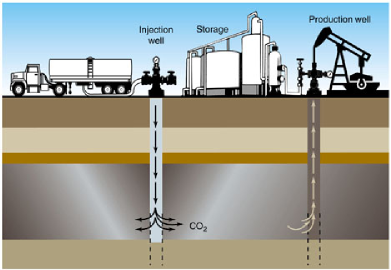
Figure 1. A schematic diagram of enhanced oil recovery. This picture is taken from https://www.llnl.gov/str/November01/Kirkendall.html.

Despite experimental evidence of viscosity depending on pressure in an exponential manner, none of the studies of technologically important applications like enhanced oil recovery (EOR) and Carbon sequestration take such a dependence on pressure into account. Enhanced oil recovery (which is also referred to as tertiary or improved oil recovery) is employed after primary and secondary methods of oil recovery, which amount to only 20-40% of oil recovery. Using EOR techniques an additional $30\%$ of oil can be obtained. One of the popular methods of enhanced oil recovery is gas injection. In the gas injection method, gas (typically, Carbon dioxide) is pumped into injection wells at high pressures, which pushes the oil to the surface at ejection wells. A typical enhanced oil recovery process is depicted in Figure 1. In a subsequent section, using a typical reservoir simulation, we will show that the results (pressure, pressure gradients, and total flow rate) obtained by taking into account the exponential dependence of viscosity on pressure are qualitatively and quantitatively different from the classical results. To this end, we consider modifying Darcy’s equation to take into account the effect of pressure on viscosity. The resulting boundary value problem is solved using a stabilized mixed method.

1.1. Stabilized mixed finite element formulations

Numerical methods for Darcy-type equations can be classified into two main categories - primal (or single-field) formulations, and mixed (or two-field) formulations. In a primal formulation, the whole problem is written in terms of the pressure (which is considered as the primary variable). The governing equation will then be a Poisson’s equation in terms of the pressure, and one can employ any of the standard numerical methods (for example, the Galerkin finite element formulation) to solve the resulting equation. Once the pressure field has been calculated, the velocity can be calculated using Darcy’s equation by using the gradient of the pressure field. The two main disadvantages of using a primal formulation have been thoroughly discussed in the literature (for example, see [7, 8]). Firstly, for low-order finite elements (which are often employed for generating complex meshes) the velocity is poorly approximated as one has to take the gradient of the pressure to calculate the velocity. In many situations, velocity is of primary interest. Secondly, primal formulations do not possess local mass conservation property with respect to the original computational grid.

On the other hand, mixed formulations can alleviate the drawbacks of primal formulations, and are widely used in many numerical simulations. Some of the earlier works on mixed methods applied to flows through porous media are [9, 10, 11, 12, 13, 14, 8, 15, 16, 17, 18]. However, it is well-known that care should be taken when dealing with mixed formulations. A mixed formulation should meet the inp-sup (also known as LBB) stability condition [19, 20]. This falls in the realm of stabilized formulations. A huge volume of literature is available on stabilized formulations for various equations (e.g., Darcy’s equation, Stokes’ flow, incompressible Navier-Stokes). A thorough discussion of stabilized methods is beyond the scope of this paper. An interested reader should refer to [21, 22, 23, 24, 25, 26, 27, 28, 29, 8, 30, 17, 31] and references therein, and to the following texts concerning stabilized methods [32, 33].

1.2. Main contributions of this paper

Some of the main contributions of this paper are

• develop a new stabilized mixed finite element formulation for the modified Darcy’s equation wherein the drag coefficient (which depends on the viscosity) is a function of pressure,

• document that the dependence of viscosity on the pressure could have a significant effect on the nature of the solution (both velocity and pressure fields), and

• stress the need and importance of better models than Darcy’s equation for modeling technologically important problems like enhanced oil recovery and Carbon sequestration for which Darcy’s equation is physically not appropriate.

1.3. An outline of the paper

The remainder of the paper is organized as follows. In Section 2 we derive Darcy’s equation and our modification of Darcy’s equation using mixture theory. In Section 3 we clearly outline our modifications to Darcy’s equation. In Section 4 we present a stabilized mixed weak formulation for our modification of Darcy’s equation, and also present a numerical solution procedure based on a consistent Newton-Raphson strategy. Representative numerical results are presented in Section 5, and conclusions are drawn in Section 6.

2. ASSUMPTIONS BEHIND DARCY’S EQUATION AND MODIFIED DARCY’S EQUATION

We now derive Darcy’s equation using mixture theory (which is also referred to as the theory of interacting continua) [34, 35, 36, 37]. This derivation reveals the main assumptions behind Darcy’s approximation, and clearly demonstrates the range of its (in)applicability. Later, we will also derive a modification of Darcy’s equation by relaxing one of the assumptions behind Darcy’s equation. We first present the balance laws in mixture theory, and then consider the flow of a fluid through a (porous) solid. It should be noted that, unless explicitly stated, repeated indices do not imply summation.

2.1. Derivation of modified Darcy equations

Consider a mixture of $N$ constituents. Let $\rho^{(i)}$ and $\boldsymbol{v}^{(i)}$, respectively, denote the density and velocity of the $i$-th constituent. The density of the mixture is defined as

(6) $$\rho=\sum_{i=1}^{N}\rho^{(i)}$$

The average velocity for the mixture (which is also referred to as the mixture velocity) is defined through

(7) $$\boldsymbol{v}=\frac{1}{\rho}\sum_{i=1}^{N}\rho^{(i)}\boldsymbol{v}^{(i)}$$

It should be noted that a variety of “mixture velocities” can be defined, and equation (7) is one of those possibilities. A detailed discussion about this important assumption and its implications with regard to the governing equations for mixture can be found in Rajagopal [38], and Rajagopal and Tao [37]. Let $\boldsymbol{T}^{(i)}$ denote the partial stress of the $i$-th constituent. The total stress is defined through

(8) $$\boldsymbol{T}=\sum_{i=1}^{N}\boldsymbol{T}^{(i)}$$

The total stress can also be defined in several ways, for a discussion of the same see Rajagopal and Tao [37]. The balance of mass can be written as

(9) $$\frac{\partial\rho^{(i)}}{\partial t}+\mathrm{div}[\rho^{(i)}\boldsymbol{v}^{(i)}]=m^{(i)}\quad\forall i$$

where $m^{(i)}$ denotes the mass production of the $i$-th constituent. The balance of mass for the mixture as a whole warrants that

(10) $$\sum_{i=1}^{N}m^{(i)}=0$$

The balance of linear momentum for the $i$-th constituent can be written as

(11) $$\rho^{(i)}\left(\frac{\partial\boldsymbol{v}^{(i)}}{\partial t}+\mathrm{grad}[\boldsymbol{v}^{(i)}]\boldsymbol{v}^{(i)}\right)=\mathrm{div}[{\boldsymbol{T}^{(i)}}^{T}]+\rho^{(i)}\boldsymbol{b}^{(i)}+\boldsymbol{I}^{(i)}$$

where $\boldsymbol{b}^{(i)}$ is the external body force acting on the $i$-th component, and $\boldsymbol{I}^{(i)}$ denotes the interaction force that is exerted by other constituents on the $i$-th constituent in virtue of their being forced to co-occupy the domain of the mixture. By Newton’s third law we have

(12) $$\sum_{i=1}^{N}\left(\boldsymbol{I}^{(i)}+m^{(i)}\boldsymbol{v}^{(i)}\right)=\boldsymbol{0}$$

It is important to note that specification of $\boldsymbol{I}^{(i)}$ is also part of the constitutive assumptions. In the absence of supply of angular momentum the balance of angular momentum can be written as

(13) $$\sum_{i=1}^{N}\boldsymbol{T}^{(i)}=\left(\sum_{i=1}^{N}\boldsymbol{T}^{(i)}\right)^{T}$$

which basically states that the total stress is symmetric. It should be noted that even in the absence of angular momentum supply the individual partial stresses $\boldsymbol{T}^{(i)}$ need not be symmetric.

We now consider the case of a mixture consisting of two constituents, namely, a fluid and a solid. The quantities associated with the solid and fluid have superscripts ‘s’ and ‘f’, respectively. The assumptions behind Darcy’s equation and their consequences are as follows:

1. No mass production of individual constituents. That is,

   (14) $$m^{(s)}=m^{(f)}=0$$

2. The solid is assumed to be a rigid porous media. Thus, one can ignore all balance laws for the solid. The stresses in the solid are what they need to be to ensure that the balance of linear momentum in the solid is met.

3. The flow is assumed to be steady

   (15) $$\frac{\partial\rho^{(f)}}{\partial t}=0\quad\mathrm{and}\quad\frac{\partial\boldsymbol{v}^{(f)}}{\partial t}=\boldsymbol{0}$$

4. The fluid is assumed to be homogeneous and incompressible. Therefore,

   (16) $$\mathrm{grad}[\rho^{(f)}]=\boldsymbol{0}\quad\mathrm{and}\quad\mathrm{div}[\boldsymbol{v}^{(f)}]=0$$

5. The velocity and its gradient are assumed to be small so that the inertial effects can be neglected, which implies that

   (17) $$\mathrm{grad}[\boldsymbol{v}^{(f)}]\boldsymbol{v}^{(f)}=\boldsymbol{0}$$

6. The partial stress in the fluid is that for an Euler fluid (that is, viscous effects within the fluid are neglected), and the partial stress takes the form

   (18) $$\boldsymbol{T}^{(f)}=-p^{(f)}\boldsymbol{I}$$

7. The only interaction force that comes into play is the frictional force at the boundaries of the pore. It is further assumed that this force is proportional to the relative velocity between the fluid and solid that is reflected by a drag-like term. Noting the fact that the solid is assumed to be rigid, and attaching the inertial frame to the solid, we have $\boldsymbol{v}^{(s)}=\boldsymbol{0}$. Hence, the interaction force on the fluid takes the form

   (19) $$\boldsymbol{I}^{(f)}=\alpha\;(\boldsymbol{v}^{(s)}-\boldsymbol{v}^{(f)})=-\alpha\boldsymbol{v}^{(f)}$$

   The drag coefficient $\alpha$, in general, can depend on pressure and relative velocity, $\boldsymbol{v}^{(s)}-\boldsymbol{v}^{(f)}$.

8. The drag coefficient $\alpha$ is independent of pressure and relative velocity, $\boldsymbol{v}^{(s)}-\boldsymbol{v}^{(f)}$.

Remark 1.

In Darcy’s equation the drag function is equal to the ratio of the viscosity of the fluid and the coefficient of permeability of the porous medium. That is,

(20) $$\alpha=\frac{\mu}{k}$$

where $k$ is the coefficient of permeability.

The above eight assumptions lead to Darcy’s equation along with the incompressibility constraint

(21a) $$\alpha\boldsymbol{v}^{(f)}+\mathrm{grad}[p^{(f)}]=\rho\boldsymbol{b}^{(f)}$$

(21b) $$\mathrm{div}[\boldsymbol{v}^{(f)}]=0$$

Remark 2.

One can obtain the Darcy-Forchheimer flow model [39] by relaxing the last assumption and allowing the drag coefficient to be a function of the magnitude of the relative velocity. Specifically, $\alpha=\alpha_{0}+\alpha_{1}\|\boldsymbol{v}^{(f)}\|$, where $\alpha_{0}$ and $\alpha_{1}$ are constants, and $\|\cdot\|$ is the 2-norm (or the Frobenius norm). Note that we have used the fact that $\boldsymbol{v}^{(s)}=\boldsymbol{0}$, and hence the magnitude of the relative velocity is equal to $\|\boldsymbol{v}^{(f)}\|$.

In the next section, we shall relax one of the assumptions behind Darcy’s equation by taking into account the dependence of viscosity on the pressure, and obtain a modification to Darcy’s equation. We shall then show that even under this small (but realistic) extension, the response of the fluid is dramatically different to the the response of the fluid obtained using Darcy’s equation. However, it should be notes that the framework offered by theory of interacting continua is quite general, and one can accommodate various aspects like mechanical deformation of the solid, thermal effects. In our future works, we shall show systematically how the response of various components in the mixture change by relaxing various other assumptions under Darcy’s equation.

3. GOVERNING EQUATIONS (MODIFIED DARCY EQUATION)

The (spatial) position vector is denoted as $\boldsymbol{x}$, and the gradient and divergence operators with respect to $\boldsymbol{x}$ are denoted as “$\mathrm{grad}$” and “$\mathrm{div}$”, respectively. Let $\Omega\subset\mathbb{R}^{nd}$ be a bounded open domain, where “$nd$” denotes the number of spatial dimensions. The boundary of $\Omega$ is denoted as $\Gamma$, which is assumed to be piecewise smooth. Mathematically, $\Gamma$ is defined as $\Gamma:=\bar{\Omega}-\Omega$, where $\bar{\Omega}$ is the closure of $\Omega$. We shall denote the velocity vector field as $\boldsymbol{v}(\boldsymbol{x})$. The pressure and density fields are denoted as $p(\boldsymbol{x})$ and $\rho(\boldsymbol{x})$, respectively.

As usual, $\Gamma$ is divided into two parts, denoted by $\Gamma^{\mathrm{D}}$ and $\Gamma^{\mathrm{N}}$, such that $\Gamma^{\mathrm{D}}\cap\Gamma^{\mathrm{N}}=\emptyset$ and $\Gamma^{\mathrm{D}}\cup\Gamma^{\mathrm{N}}=\Gamma$. $\Gamma^{\mathrm{N}}$ is the part of the boundary on which normal component of the velocity is prescribed, and $\Gamma^{\mathrm{D}}$ is part of the boundary on which pressure is prescribed. The modified Darcy equations can be written as

(22a) $$\alpha(p)\boldsymbol{v}+\mathrm{grad}[p]=\rho\boldsymbol{b}\quad\mbox{in}\;\Omega$$

(22b) $$\mathrm{div}[\boldsymbol{v}]=0\quad\mbox{in}\;\Omega$$

(22c) $$\boldsymbol{v}(\boldsymbol{x})\cdot\boldsymbol{n}(\boldsymbol{x})=v_{n}(\boldsymbol{x})\quad\mbox{on}\;\Gamma^{\mathrm{N}}$$

(22d) $$p(\boldsymbol{x})=p_{0}(\boldsymbol{x})\quad\mbox{on}\;\Gamma^{\mathrm{D}}$$

where $\alpha(p)$ (which has dimension of $\left[\mathrm{M}\mathrm{L}^{-3}\mathrm{T}^{-1}\right]$) is the drag function, $p_{0}(\boldsymbol{x})$ is the prescribed pressure, $v_{n}(\boldsymbol{x})$ is the prescribed normal component of the velocity, $\boldsymbol{b}(\boldsymbol{x})$ is the specific body force, and $\boldsymbol{n}(\boldsymbol{x})$ is the unit outward normal vector to $\Gamma$.

Remark 3.

If $\Gamma^{\mathrm{N}}=\Gamma$ then for well-posedness of (22) one needs to satisfy the following compatibility condition

(23) $$\int_{\Gamma^{\mathrm{N}}=\Gamma}v_{n}\;\mathrm{d}\Gamma=0$$

which is a direct consequence of the divergence theorem. Also in this case, the solution for pressure is not unique. For uniqueness of the solution one needs to impose an additional constraint on the pressure. For example,

(24) $$\int_{\Omega}p\;\mathrm{d}\Omega=0$$

In numerical simulations, it is common to prescribe the pressure at a point, which is computationally easier than enforcing the constraint (24).

In this paper we consider the following three different drag functions

(25a) $$\alpha(p)=\alpha_{0}$$

(25b) $$\alpha(p)=\alpha_{0}\left(1+\beta p\right)$$

(25c) $$\alpha(p)=\alpha_{0}\exp\left[\beta p\right]$$

where $\alpha_{0}>0$ and $\beta>0$ are constants independent of $p$, $\boldsymbol{v}$ and $\rho$ but can be functions of $\boldsymbol{x}$. The dimension of the coefficient $\beta$ is $\left[\mathrm{M}^{-1}\mathrm{L}\mathrm{T}^{-2}\right]$. The constant drag function (25a) gives rise to (standard) Darcy’s equation, and the drag function (25b) is based on Barus’ formula (1). Note that as $p\rightarrow\infty$ the drag coefficient (25a) $\frac{\alpha(p)}{p}\rightarrow 0$, drag coefficient (25b) $\frac{\alpha(p)}{p}\rightarrow\alpha_{0}\beta$ (a constant), and drag coefficient (25c) $\frac{\alpha(p)}{p}\rightarrow\infty$.

Several rigorous mathematical studies have addressed the equations governing the flows of fluids with pressure dependent viscosity. Existence of solutions have been established recently by Málek et al. [40], Hron et al. [41], Franta et al. [42], and Buliček et al. [43]. However, it is important to note that all the aforementioned existence results have been established under the condition $\frac{\mu}{p}\rightarrow\mathrm{constant}$ as $p\rightarrow\infty$. But, experiments suggest that $\frac{\mu}{p}\rightarrow\infty$ as $p\rightarrow\infty$ (for example, Barus’ formula). Thus, rigorous results such as existence of solutions for fluids with pressure dependent viscosity are open with regard to the type of variation of the viscosity with pressure observed in experiments.

It is, in general, not possible to obtain analytical solutions for the above boundary value problem (22). One has to resort to numerical solutions to solve realistic problems on complex domains. In this paper we employ the Finite Element Method (FEM), which is a powerful and systematic technique for numerically solving partial differential equations. To this end, we present the classical mixed formulation, and then present a new stabilized mixed formulation for solving modified Darcy equations.

3.1. Classical mixed formulation

Let $L^{2}(\Omega)$ be the space of square integrable (scalar) functions on $\Omega$, and $\mathbf{L}^{2}(\Omega)$ be space of square integrable vector fields defined on $\Omega$. For convenience, we denote the $L^{2}$ inner-product over a spatial domain, $K$, as

(26a) $$(a;b)_{K}=\int_{K}a\cdot b\;\mathrm{d}K\quad\forall a,b\in L^{2}(K)$$

(26b) $$(\boldsymbol{a};\boldsymbol{b})_{K}=\int_{K}\boldsymbol{a}\cdot\boldsymbol{b}\;\mathrm{d}K\quad\forall\boldsymbol{a},\boldsymbol{b}\in\mathbf{L}^{2}(K)$$

The subscript $K$ will be dropped if $K$ is the whole of $\Omega$, that is $K=\Omega$. The (Hilbert) spaces $H^{1}(\Omega)$ and $\mathbf{H}(\mathrm{div},\Omega)$ are, respectively, defined as

(27a) $$H^{1}(\Omega) :=\left\{a(\boldsymbol{x})\in L^{2}(\Omega)\;\big{|}\;\mathrm{grad}[a]\in\mathbf{L}^{2}(\Omega)\right\}$$

(27b) $$\mathbf{H}(\mathrm{div},\Omega) :=\left\{\boldsymbol{a}(\boldsymbol{x})\in\mathbf{L}^{2}(\Omega)\;\big{|}\;\mathrm{div}[\boldsymbol{a}]\in L^{2}(\Omega)\right\}$$

Furthermore, we shall define the following function spaces

(28a) $$\mathcal{V}:=\left\{\boldsymbol{v}(\boldsymbol{x})\in\mathbf{H}(\mathrm{div},\Omega)\;\big{|}\;\mathrm{trace}\left[\boldsymbol{v}(\boldsymbol{x})\cdot\boldsymbol{n}(\boldsymbol{x})\right]=v_{n}(\boldsymbol{x})\;\mathrm{on}\;\Gamma^{\mathrm{N}}\right\}$$

(28b) $$\mathcal{W}:=\left\{\boldsymbol{w}(\boldsymbol{x})\in\mathbf{H}(\mathrm{div},\Omega)\;\big{|}\;\mathrm{trace}\left[\boldsymbol{w}(\boldsymbol{x})\cdot\boldsymbol{n}(\boldsymbol{x})\right]=0\;\mathrm{on}\;\Gamma^{\mathrm{N}}\right\}$$

(28c) $$\mathcal{P}\equiv L^{2}(\Omega),\quad\mathcal{Q}\equiv H^{1}(\Omega)$$

where $\mathrm{trace}[\cdot]$ is the standard trace operator [20].

The classical mixed formulation for the modified Darcy equation (22) can be written as: Find $\boldsymbol{v}(\boldsymbol{x})\in\mathcal{V}$ and $p(\boldsymbol{x})\in\mathcal{P}$ such that

(29) $$(\boldsymbol{w};\alpha(p)\boldsymbol{v})-(\mathrm{div}[\boldsymbol{w}];p)+(\boldsymbol{w}\cdot\boldsymbol{n};p_{0})_{\Gamma^{\mathrm{D}}}-(q;\mathrm{div}[\boldsymbol{v}])=(\boldsymbol{w};\rho\boldsymbol{b})\quad\forall\boldsymbol{w}(\boldsymbol{x})\in\mathcal{W},\;q(\boldsymbol{x})\in\mathcal{P}$$

Assuming the domain and boundary are sufficiently smooth, for the case of constant drag function the above weak formulation (29) is well-posed [20]. A corresponding finite element formulation can be obtained by choosing suitable approximating finite element spaces, which (for a conforming formulation) will be finite dimensional subspaces of the underlying function spaces of the weak formulation. Let the finite element function spaces for the velocity, the weighting function associated with the velocity, and the pressure be denoted by $\mathcal{V}^{h}\subset\mathcal{V}$, $\mathcal{W}^{h}\subset\mathcal{W}$, and $\mathcal{P}^{h}\subset\mathcal{P}$, respectively. A conforming finite element formulation of the classical mixed formulation reads: Find $\boldsymbol{v}^{h}(\boldsymbol{x})\in\mathcal{V}^{h}$ and $p^{h}(\boldsymbol{x})\in\mathcal{P}^{h}$ such that

(30) $$(\boldsymbol{w}^{h};\alpha(p^{h})\boldsymbol{v}^{h})-(\mathrm{div}[\boldsymbol{w}^{h}];p^{h})+(\boldsymbol{w}^{h}\cdot\boldsymbol{n};p_{0})_{\Gamma^{\mathrm{D}}}-(q^{h};\mathrm{div}[\boldsymbol{v}^{h}])=(\boldsymbol{w}^{h};\rho\boldsymbol{b})\quad\forall\boldsymbol{w}^{h}(\boldsymbol{x})\in\mathcal{W}^{h},\;q^{h}(\boldsymbol{x})\in\mathcal{P}^{h}$$

For mixed formulations, the inclusions $\mathcal{V}^{h}\subset\mathcal{V}$, $\mathcal{W}^{h}\subset\mathcal{W}$, and $\mathcal{P}^{h}\subset\mathcal{P}$ are themselves not sufficient to produce stable results, and additional conditions must be met by the members of these finite element spaces to obtain meaningful numerical results. A systematic study of these types of conditions on function spaces to obtain stable numerical results is the main theme of mixed finite elements. One of the main conditions to be met is the Ladyzhenskaya-Babuška-Brezzi (LBB) inf-sup stability condition. For further details, see references [20, 44].

It is well-known that under the classical mixed formulation many combinations of interpolations for velocity and pressure produce spurious oscillations (in the pressure field) when applied to problems involving incompressibility as a constraint [20, 44]. In particular, the equal-order interpolation for the velocity and pressure (which is computationally the most convenient) does not satisfy the LBB condition, and produces spurious oscillations in the pressure field. However, elegant solutions for approximating the velocity and pressure that are stable under the classical mixed formulation have been proposed [45, 46, 47, 48, 49, 50]. These discrete spaces have been successfully used in many numerical simulations, and good accuracy has been attained in both the velocity and pressure fields. But a computer implementation of these methods is more involved because of different interpolations for the velocity and pressure.

In the next section we present a new stabilized mixed formulation for modified Darcy equations under which the computationally convenient equal-order interpolation for velocity and pressure is stable.

4. A STABILIZED MIXED FORMULATION

A variational multiscale mixed formulation has been proposed and studied by Hughes and Masud [8] and Nakshatrala et al. [17] for Darcy’s equation. In reference [17] it has been shown that this variational multiscale formulation for Darcy’s equation passes three-dimensional patch tests even for distorted meshes, and performs well even on complex geometries with unstructured meshes. In this paper we extend this formulation to the modifications to Darcy’s equation developed in this paper.

A stabilized mixed formulation for modified Darcy’s equation (22) can be written as: Find $\boldsymbol{v}(\boldsymbol{x})\in\mathcal{V}$ and $p(\boldsymbol{x})\in\mathcal{Q}$ such that

$$\left(\boldsymbol{w};\alpha(p)\boldsymbol{v}\right) -\left(\mathrm{div}[\boldsymbol{w}];p\right)+\left(\boldsymbol{w}\cdot\boldsymbol{n};p_{0}\right)_{\Gamma^{\mathrm{D}}}-\left(q;\mathrm{div}[\boldsymbol{v}]\right)-\left(\boldsymbol{w};\rho\boldsymbol{b}\right)$$

(31) $$-\frac{1}{2}\left(\alpha(p)\boldsymbol{w}+\mathrm{grad}[q];\alpha^{-1}(p)\left(\alpha(p)\boldsymbol{v}+\mathrm{grad}[p]-\rho\boldsymbol{b}\right)\right)=0\quad\forall\boldsymbol{w}(\boldsymbol{x})\in\mathcal{W},\;q(\boldsymbol{x})\in\mathcal{Q}$$

The terms in the first line of equation (4) are from the classical mixed formulation, and the terms in the second line are the stabilization terms. The factor $1/2$ on the second line is the stabilization parameter, which is determined neither by mesh-dependent parameters nor on material properties (like viscosity). The stabilization term is based on the residual of the modified Darcy’s equation (22). Similarly, one may add a residual-based term using the incompressibility constraint, which in some cases improves stability (e.g., see [8]). We now solve the above weak formulation (4) using the Finite Element Method.

4.1. A finite element approximation

Let the domain $\Omega$ be decomposed into “$Nele$” non-overlapping open element subdomains. That is,

(32) $$\bar{\Omega}=\bigcup_{e=1}^{Nele}\bar{\Omega}^{e}$$

where a superposed bar denotes closure. The boundary of $\Omega^{e}$ is denoted as $\partial\Omega^{e}:=\bar{\Omega}^{e}-\Omega^{e}$. For a non-negative integer $m$, $\mathcal{P}^{m}(\Omega^{e})$ denotes the linear vector space spanned by polynomials up to $m$th order defined on the subdomain $\Omega^{e}$. We shall define the following finite dimensional vector spaces of $\mathcal{V}$, $\mathcal{W}$ and $\mathcal{Q}$:

(33a) $$\mathcal{V}^{h} :=\left\{\boldsymbol{v}^{h}(\boldsymbol{x})\in\mathcal{V}\;\big{|}\;\boldsymbol{v}^{h}(\boldsymbol{x})\in\left(C^{0}(\bar{\Omega})\right)^{nd},\boldsymbol{v}^{h}(\boldsymbol{x})\big{|}_{\Omega^{e}}\in\left(\mathcal{P}^{k}(\Omega^{e})\right)^{nd},e=1,\cdots,Nele\right\}$$

(33b) $$\mathcal{W}^{h} :=\left\{\boldsymbol{w}^{h}(\boldsymbol{x})\in\mathcal{W}\;\big{|}\;\boldsymbol{w}^{h}(\boldsymbol{x})\in\left(C^{0}(\bar{\Omega})\right)^{nd},\boldsymbol{w}^{h}(\boldsymbol{x})\big{|}_{\Omega^{e}}\in\left(\mathcal{P}^{k}(\Omega^{e})\right)^{nd},e=1,\cdots,Nele\right\}$$

(33c) $$\mathcal{Q}^{h} :=\left\{p^{h}(\boldsymbol{x})\in\mathcal{Q}\;\big{|}\;p^{h}(\boldsymbol{x})\in C^{0}(\bar{\Omega}),p^{h}(\boldsymbol{x})\big{|}_{\Omega^{e}}\in\mathcal{P}^{l}(\Omega^{e}),e=1,\cdots,Nele\right\}$$

where $k$ and $l$ are non-negative integers, and recall that “$nd$” denotes the number of spatial dimensions. A corresponding finite element formulation can be written as: Find $\boldsymbol{v}^{h}(\boldsymbol{x})\in\mathcal{V}^{h}$ and $p^{h}(\boldsymbol{x})\in\mathcal{Q}^{h}$ such that

$$(\boldsymbol{w}^{h};\alpha(p^{h})\boldsymbol{v}^{h})-(\mathrm{div}[\boldsymbol{w}^{h}];p^{h})+(\boldsymbol{w}^{h}\cdot\boldsymbol{n};p_{0})_{\Gamma^{\mathrm{D}}}-(q^{h};\mathrm{div}[\boldsymbol{v}^{h}])-(\boldsymbol{w}^{h};\rho\boldsymbol{b})$$

(34) $$-\frac{1}{2}\left(\alpha(p^{h})\boldsymbol{w}^{h}+\mathrm{grad}[q^{h}];\alpha^{-1}(p^{h})(\alpha(p^{h})\boldsymbol{v}^{h}+\mathrm{grad}[p^{h}]-\rho\boldsymbol{b})\right)=0\quad\forall\boldsymbol{w}^{h}\in\mathcal{W}^{h},\;q^{h}\in\mathcal{Q}^{h}$$

Due to the presence of the term $\frac{1}{2}(\mathrm{grad}[q^{h}];\alpha^{-1}(p^{h})\mathrm{grad}[p^{h}])$, the above formulation circumvents the LBB condition, and hence one can employ equal-order interpolation for velocity and pressure, which will be confirmed by numerical results presented in a subsequent section.

We solve the resulting nonlinear equations based on a consistent Newton-Raphson solution procedure. We now derive corresponding residual vector and tangent matrix, which are required for such a procedure.

4.2. Residual vector

We shall define the nodal unknowns for the velocity (denoted as $\hat{\boldsymbol{v}}_{e}$) and pressure (denoted as $\hat{\boldsymbol{p}}_{e}$) for a given element $\Omega^{e}$ as

(41) $$\hat{\boldsymbol{v}}_{e}:=\left[\begin{array}[]{ccc}v_{1,1}&\cdots&v_{1,nd}\\ \vdots&\ddots&\vdots\\ v_{n,1}&\cdots&v_{n,nd}\end{array}\right],\quad\hat{\boldsymbol{p}}_{e}:=\left[\begin{array}[]{c}p_{1}\\ \vdots\\ p_{n}\end{array}\right]$$

where $n$ is the number of nodes in the given element, and $nd$ (as mentioned earlier) is the number of spatial dimensions. The solution, $\boldsymbol{v}(\boldsymbol{x})$ and $p(\boldsymbol{x})$, over the element $\Omega^{e}$ are interpolated in terms of corresponding nodal values (which have a superposed hat) as

(42) $$\boldsymbol{v}(\boldsymbol{x})=\hat{\boldsymbol{v}}^{T}_{e}\boldsymbol{N}^{T}(\boldsymbol{x}),\quad p(\boldsymbol{x})=\boldsymbol{N}(\boldsymbol{x})\hat{\boldsymbol{p}}_{e}$$

where $\boldsymbol{N}(\boldsymbol{x})$ is a row vector of shape functions. Likewise, the weighting functions, $\boldsymbol{w}(\boldsymbol{x})$ and $q(\boldsymbol{x})$, over an element are interpolated as

(43) $$\boldsymbol{w}(\boldsymbol{x})=\hat{\boldsymbol{w}}^{T}_{e}\boldsymbol{N}^{T}(\boldsymbol{x}),\quad q(\boldsymbol{x})=\boldsymbol{N}(\boldsymbol{x})\hat{\boldsymbol{q}}_{e}$$

where the nodal (arbitrary) weights $\hat{\boldsymbol{w}}_{e}$ and $\hat{\boldsymbol{q}}_{e}$ are defined similar to $\hat{\boldsymbol{v}}_{e}$ and $\hat{\boldsymbol{p}}_{e}$ (which are defined in equation (41)). One can construct residual vectors corresponding to equation (4) by substituting equations (42) into equation (4), and invoking the arbitrariness of $\hat{\boldsymbol{w}}_{e}$ and $\hat{\boldsymbol{q}}_{e}$. The element residual vectors can be written as

$$\boldsymbol{R}^{e}_{v}(\hat{\boldsymbol{v}}_{e},\hat{\boldsymbol{p}}_{e}) :=\int_{\Omega^{e}}(\boldsymbol{N}^{T}\odot\boldsymbol{I})\alpha(p)\boldsymbol{v}\;\mathrm{d}\Omega-\int_{\Omega^{e}}\mathrm{vec}\left[\boldsymbol{B}^{T}\right]p\;\mathrm{d}\Omega+\int_{\partial\Omega^{e}\cap\Gamma^{\mathrm{D}}}(\boldsymbol{N}^{T}\odot\boldsymbol{I})\boldsymbol{n}p_{0}\;\mathrm{d}\Gamma$$

(44) $$-\int_{\Omega^{e}}(\boldsymbol{N}^{T}\odot\boldsymbol{I})\rho\boldsymbol{b}\;\mathrm{d}\Omega-\frac{1}{2}\int_{\Omega^{e}}(\boldsymbol{N}^{T}\odot\boldsymbol{I})\left(\alpha(p)\boldsymbol{v}+\mathrm{grad}[p]-\rho\boldsymbol{b}\right)\;\mathrm{d}\Omega$$

(45) $$\boldsymbol{R}^{e}_{p}(\hat{\boldsymbol{v}}_{e},\hat{\boldsymbol{p}}_{e}) :=-\int_{\Omega^{e}}\boldsymbol{N}^{T}\mathrm{div}[\boldsymbol{v}]\;\mathrm{d}\Omega-\frac{1}{2}\int_{\Omega^{e}}\boldsymbol{B}\;\alpha^{-1}(p)\left(\alpha(p)\boldsymbol{v}+\mathrm{grad}[p]-\rho\boldsymbol{b}\right)\;\mathrm{d}\Omega$$

where $\boldsymbol{v}$ and $p$ are approximated using equation (42), $\mathrm{vec}[\cdot]$ is an operation that represents a matrix as a vector, $\odot$ is Kronecker product [51] (see Appendix 7), $\boldsymbol{B}:=\boldsymbol{DN}\boldsymbol{J}^{-1}$, $\boldsymbol{J}:=\partial\boldsymbol{x}/\partial\boldsymbol{\xi}$ is the element Jacobian matrix, $\boldsymbol{DN}$ represents a matrix of (first) derivatives of element shape functions with respect to reference coordinates $\boldsymbol{\xi}$. For example, for a three-node triangular element the matrix $\boldsymbol{DN}$ will read

(49) $$\boldsymbol{DN} :=\left[\begin{array}[]{cc}\frac{\partial N_{1}}{\partial\xi_{1}}&\frac{\partial N_{1}}{\partial\xi_{2}}\\ \vdots&\vdots\\ \frac{\partial N_{3}}{\partial\xi_{1}}&\frac{\partial N_{3}}{\partial\xi_{2}}\end{array}\right]$$

We shall define the global unknown vectors $\hat{\boldsymbol{v}}$ and $\hat{\boldsymbol{p}}$ as

(56) $$\hat{\boldsymbol{v}}:=\left[\begin{array}[]{ccc}v_{1,1}&\cdots&v_{1,nd}\\ \vdots&\ddots&\vdots\\ v_{nn,1}&\cdots&v_{nn,nd}\end{array}\right],\quad\hat{\boldsymbol{p}}:=\left[\begin{array}[]{c}p_{1}\\ \vdots\\ p_{nn}\end{array}\right]$$

where $nn$ denotes the total number of nodes in the finite element mesh. Global residual vectors can be constructed from element residual vectors using the standard assembly procedure

(57) $$\boldsymbol{R}_{v}(\hat{\boldsymbol{v}},\hat{\boldsymbol{p}})={\huge\boldsymbol{\mathsf{A}}}_{e=1}^{Nele}\boldsymbol{R}^{e}_{v}(\hat{\boldsymbol{v}}_{e},\hat{\boldsymbol{p}}_{e}),\quad\boldsymbol{R}_{p}(\hat{\boldsymbol{v}},\hat{\boldsymbol{p}})={\huge\boldsymbol{\mathsf{A}}}_{e=1}^{Nele}\boldsymbol{R}^{e}_{p}(\hat{\boldsymbol{v}}_{e},\hat{\boldsymbol{p}}_{e})$$

where ${\huge\boldsymbol{\mathsf{A}}}$ is the standard assembly operator [52]. (Recall that $Nele$ denotes the number of elements.) The finite element solution can be obtained by solving simultaneously

(58) $$\boldsymbol{R}_{v}(\hat{\boldsymbol{v}},\hat{\boldsymbol{p}})=\boldsymbol{0}\;\mathrm{and}\;\boldsymbol{R}_{p}(\hat{\boldsymbol{v}},\hat{\boldsymbol{p}})=\boldsymbol{0}$$

4.3. Tangent matrix

Using a Newton-Raphson type approach, one can obtain the solution in an iterative fashion using the following update equation until the residual is under a prescribed tolerance

(59a) $$\mathrm{vec}\left[\hat{\boldsymbol{v}}^{(i+1)}\right]=\mathrm{vec}\left[\hat{\boldsymbol{v}}^{(i)}\right]+\mathrm{vec}\left[\Delta\hat{\boldsymbol{v}}^{(i)}\right]$$

(59b) $$\mathrm{vec}\left[\hat{\boldsymbol{p}}^{(i+1)}\right]=\mathrm{vec}\left[\hat{\boldsymbol{p}}^{(i)}\right]+\mathrm{vec}\left[\Delta\hat{\boldsymbol{p}}^{(i)}\right]$$

The updates at iteration $i$ are calculated from the following system of equations

(66) $$\left[\begin{array}[]{cc}\boldsymbol{K}_{vv}&\boldsymbol{K}_{vp}\\ \boldsymbol{K}_{pv}&\boldsymbol{K}_{pp}\\ \end{array}\right]\left\{\begin{array}[]{c}\mathrm{vec}\left[\Delta\hat{\boldsymbol{v}}^{(i)}\right]\\ \mathrm{vec}\left[\Delta\hat{\boldsymbol{p}}^{(i)}\right]\\ \end{array}\right\}=-\left\{\begin{array}[]{c}\boldsymbol{R}_{v}\\ \boldsymbol{R}_{p}\\ \end{array}\right\}$$

where

(67) $$\boldsymbol{K}_{vv}={\huge\boldsymbol{\mathsf{A}}}_{e=1}^{Nele}\boldsymbol{K}^{e}_{vv},\;\boldsymbol{K}_{vp}={\huge\boldsymbol{\mathsf{A}}}_{e=1}^{Nele}\boldsymbol{K}^{e}_{vp},\;\boldsymbol{K}_{pv}={\huge\boldsymbol{\mathsf{A}}}_{e=1}^{Nele}\boldsymbol{K}^{e}_{pv},\;\boldsymbol{K}_{pp}={\huge\boldsymbol{\mathsf{A}}}_{e=1}^{Nele}\boldsymbol{K}^{e}_{pp}$$

and the element matrices are defined as

(68a) $$\boldsymbol{K}_{vv}^{e} =\frac{1}{2}\int_{\Omega^{e}}\left(\boldsymbol{N}^{T}\odot\boldsymbol{I}\right)\alpha(p)\left(\boldsymbol{N}\odot\boldsymbol{I}\right)\;\mathrm{d}\Omega$$

(68b) $$\boldsymbol{K}_{vp}^{e} =\frac{1}{2}\int_{\Omega^{e}}\left(\boldsymbol{N}^{T}\odot\boldsymbol{I}\right)\boldsymbol{v}\left(\frac{\mathrm{d}\alpha}{\mathrm{d}p}\right)\boldsymbol{N}\;\mathrm{d}\Omega-\int_{\Omega^{e}}\mathrm{vec}\left[\boldsymbol{B}^{T}\right]\boldsymbol{N}\;\mathrm{d}\Omega-\frac{1}{2}\int_{\Omega^{e}}\left(\boldsymbol{N}^{T}\odot\boldsymbol{I}\right)\boldsymbol{B}^{T}\;\mathrm{d}\Omega$$

(68c) $$\boldsymbol{K}_{pv}^{e} =-\int_{\Omega^{e}}\boldsymbol{N}^{T}\mathrm{vec}\left[\boldsymbol{B}^{T}\right]^{T}\;\mathrm{d}\Omega-\frac{1}{2}\int_{\Omega^{e}}\boldsymbol{B}\left(\boldsymbol{N}\odot\boldsymbol{I}\right)\;\mathrm{d}\Omega$$

(68d) $$\boldsymbol{K}_{pp}^{e} =-\frac{1}{2}\int_{\Omega^{e}}\boldsymbol{B}\alpha^{-1}(p)\boldsymbol{B}^{T}\;\mathrm{d}\Omega+\frac{1}{2}\int_{\Omega^{e}}\boldsymbol{B}\;\left(\mathrm{grad}[p]-\rho\boldsymbol{b}\right)\frac{1}{\alpha^{2}(p)}\left(\frac{\mathrm{d}\alpha}{\mathrm{d}p}\right)\boldsymbol{N}\;\mathrm{d}\Omega$$

Remark 4.

From equation (68) it is evident that for the modified Darcy’s equation, in general, we have ${\boldsymbol{K}_{pv}^{e}}\neq{\boldsymbol{K}_{vp}^{e}}^{T}$, and the matrix $\boldsymbol{K}_{pp}^{e}$ is not symmetric. But in the case of Darcy’s equation (for which $\alpha$ is independent of pressure) we do have $\boldsymbol{K}_{pv}^{e}={\boldsymbol{K}_{vp}^{e}}^{T}$, and the matrix $\boldsymbol{K}_{pp}^{e}$ is symmetric. It should be noted that symmetry of tangent matrix (or the lack of it) is an important factor to be considered in the selection of solvers for the resulting system of linear equations, and also in the design/selection of preconditioners for iterative solvers, which are commonly employed in large-scale problems.

5. REPRESENTATIVE NUMERICAL RESULTS

In this section, we present representative numerical results to illustrate the performance of the proposed stabilized mixed formulation. In all our numerical simulations we have employed equal-order interpolation for pressure and velocity as shown in Figure 2.

First, we shall non-dimensionalize the governing equations. To this end, we define the following non-dimensional quantities (which have a superposed bar)

(69) $$\bar{\boldsymbol{x}}=\frac{\boldsymbol{x}}{L},\;\bar{\boldsymbol{v}}=\frac{\boldsymbol{v}}{V},\;\bar{p}=\frac{p}{P},\;\bar{\alpha}=\frac{\alpha}{\alpha_{\mathrm{ref}}},\;\bar{\alpha}_{0}=\frac{\alpha_{0}}{\alpha_{\mathrm{ref}}},\;\bar{\rho}=\frac{\rho}{\rho_{\mathrm{ref}}},\;\bar{\boldsymbol{b}}=\frac{\boldsymbol{b}}{B},\;\bar{\beta}=\beta P,\;\bar{v}_{n}=\frac{v_{n}}{V},\;\bar{p}_{0}=\frac{p_{0}}{P}$$

where $L$, $V$, $P$, $\alpha_{\mathrm{ref}}$, $\rho_{\mathrm{ref}}$ and $B$ respectively denote reference length, velocity, pressure, drag coefficient, density and specific body force. The gradient and divergence operators with respect to $\bar{\boldsymbol{x}}$ are denoted as “$\overline{\mathrm{grad}}$” and “$\overline{\mathrm{div}}$”, respectively. The scaled domain $\Omega_{\mathrm{scaled}}$ is defined as follows: a point in space with position vector $\bar{\boldsymbol{x}}\in\Omega_{\mathrm{scaled}}$ corresponds to the same point with position vector given by $\boldsymbol{x}=\bar{\boldsymbol{x}}L\in\Omega$. Similarly, one can define the scaled boundaries: $\partial\Omega_{\mathrm{scaled}}$, $\Gamma^{\mathrm{D}}_{\mathrm{scaled}}$, and $\Gamma^{\mathrm{N}}_{\mathrm{scaled}}$. The above non-dimensionalization gives rise to two dimensionless parameters

(70) $$\mathcal{A}:=\frac{\alpha_{\mathrm{ref}}VL}{P},\quad\mathcal{C}:=\frac{\rho_{\mathrm{ref}}LB}{P}$$

A corresponding non-dimensionalized form of the drag functions given in equation (25) can be written as

(71a) $$\bar{\alpha}(\bar{p}) =\bar{\alpha}_{0}$$

(71b) $$\bar{\alpha}(\bar{p}) =\bar{\alpha}_{0}\left(1+\bar{\beta}\bar{p}\right)$$

(71c) $$\bar{\alpha}(\bar{p}) =\bar{\alpha}_{0}\exp[\bar{\beta}\bar{p}]$$

We shall write a non-dimensional form of the modified Darcy equation as

(72a) $$\mathcal{A}\;\bar{\alpha}(\bar{p})\bar{\boldsymbol{v}}+\overline{\mathrm{grad}}[p]=\mathcal{C}\;\bar{\rho}\;\bar{\boldsymbol{b}}\quad\;\mathrm{in}\;{\Omega}_{\mathrm{scaled}}$$

(72b) $$\overline{\mathrm{div}}[\bar{\boldsymbol{v}}]=0\quad\;\mathrm{in}\;{\Omega}_{\mathrm{scaled}}$$

(72c) $$\bar{\boldsymbol{v}}\cdot\bar{\boldsymbol{n}}=\bar{v}_{n}(\bar{\boldsymbol{x}})\quad\;\mathrm{on}\;{\Gamma}^{\mathrm{N}}_{\mathrm{scaled}}$$

(72d) $$\bar{p}(\bar{\boldsymbol{x}})=\bar{p}_{0}(\bar{\boldsymbol{x}})\quad\;\mathrm{on}\;{\Gamma}^{\mathrm{D}}_{\mathrm{scaled}}$$

where $\bar{\boldsymbol{n}}(\bar{\boldsymbol{x}})$ is the unit outward normal to the boundary $\partial{\Omega}_{\mathrm{scaled}}$.

5.1. A simple one-dimensional problem

We shall test the proposed stabilized mixed formulation using a simple one-dimensional problem, which is pictorially described in Figure 3. Pressures of $\bar{p}_{1}$ and $\bar{p}_{2}$ are respectively prescribed at the left and right ends of the unit domain, and we neglect the body force. The governing equations for this test problem can be written as

(73a) $$\mathcal{A}\bar{\alpha}(\bar{p})\bar{v}(\bar{x})+\frac{\mathrm{d}\bar{p}}{\mathrm{d}\bar{x}}=0\quad\mathrm{in}\;(0,1)$$

(73b) $$\frac{\mathrm{d}\bar{v}}{d\bar{x}}=0\quad\mathrm{in}\;(0,1)$$

(73c) $$\bar{p}(\bar{x}=0)=\bar{p}_{1},\quad\bar{p}(\bar{x}=1)=\bar{p}_{2}$$

For this test problem, the analytical solutions with the drag functions defined in equation (25) can be written as

(74c) $$\mbox{for the case}\;\bar{\alpha}(\bar{p})=\bar{\alpha}_{0}\;\left\{\begin{array}[]{l}\bar{p}(\bar{x})=\left(\bar{p}_{2}-\bar{p}_{1}\right)\bar{x}+\bar{p}_{1}\\ \bar{v}(\bar{x})=-\frac{\left(\bar{p}_{2}-\bar{p}_{1}\right)}{\mathcal{A}\bar{\alpha}_{0}}\end{array}\right.$$

(74f) $$\mbox{for the case}\;\bar{\alpha}(\bar{p})=\bar{\alpha}_{0}(1+\bar{\beta}\bar{p})\;\left\{\begin{array}[]{l}\bar{p}(\bar{x})=\frac{1}{\bar{\beta}}\left[\left(1+\bar{\beta}\bar{p}_{1}\right)^{1-\bar{x}}\left(1+\bar{\beta}\bar{p}_{2}\right)^{\bar{x}}-1\right]\\ \bar{v}(\bar{x})=\frac{-1}{\mathcal{A}\bar{\alpha}_{0}\bar{\beta}}\ln\left[\frac{1+\bar{\beta}\bar{p}_{2}}{1+\bar{\beta}\bar{p}_{1}}\right]\end{array}\right.$$

(74i) $$\mbox{for the case}\;\bar{\alpha}(\bar{p})=\bar{\alpha}_{0}\exp[\bar{\beta}\bar{p}]\;\left\{\begin{array}[]{l}\bar{p}(\bar{x})=\frac{-1}{\bar{\beta}}\ln\left\{(1-\bar{x})\exp\left[-\bar{\beta}\bar{p}_{1}\right]+\bar{x}\exp\left[-\bar{\beta}\bar{p}_{2}\right]\right\}\\ \bar{v}(\bar{x})=\frac{1}{\mathcal{A}\bar{\alpha}_{0}\bar{\beta}}\left\{\exp\left[-\bar{\beta}\bar{p}_{2}\right]-\exp\left[-\bar{\beta}\bar{p}_{1}\right]\right\}\end{array}\right.$$

In Figure 4 we compare the numerical solutions against the analytical solutions for various drag functions. In all the considered cases, the proposed numerical formulation performed well.

5.2. Five-spot problem

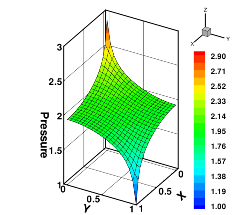
(a) Pressure contours using Darcy’s equation

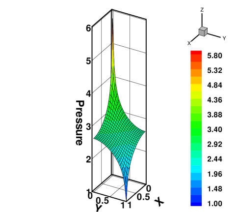
(b) Pressure contours using modified Darcy’s equation

Figure 6. Five-spot problem using $400$ four-node quadrilateral elements: This figure compares elevation plots for the pressure profile using Darcy’s equation (top) and modified Darcy’s equation (bottom). The pressure based on modified Darcy’s equation with the viscosity given by Barus’ formula exhibits steeper gradients compared to ones obtained using Darcy’s equation. As one can see there are no spurious oscillations in the pressure field despite the steep gradients in pressure near the injection and pressure wells. For Barus’ formula we have used $\alpha_{0}=1$ and $\beta=0.3$.

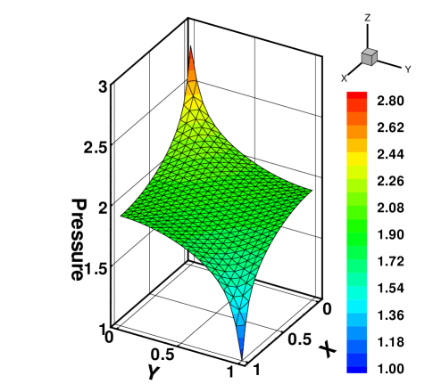
(a) Pressure contours using Darcy’s equation

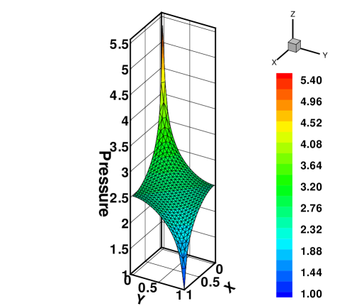
(b) Pressure contous using modified Darcy’s equation

Figure 7. Five-spot problem using $800$ three-node triangular elements: This figure compares elevation plots for the pressure profile using Darcy’s equation and modified Darcy’s equation (bottom). The pressure based on modified Darcy’s equation with the viscosity given by Barus’ formula exhibits steeper gradients compared to ones obtained using Darcy’s equation. As one can see there are no spurious oscillations in the pressure field despite the steep gradients in pressure near the injection and production wells. For Barus’ formula, we have used $\alpha_{0}=1$ and $\beta=0.3$.

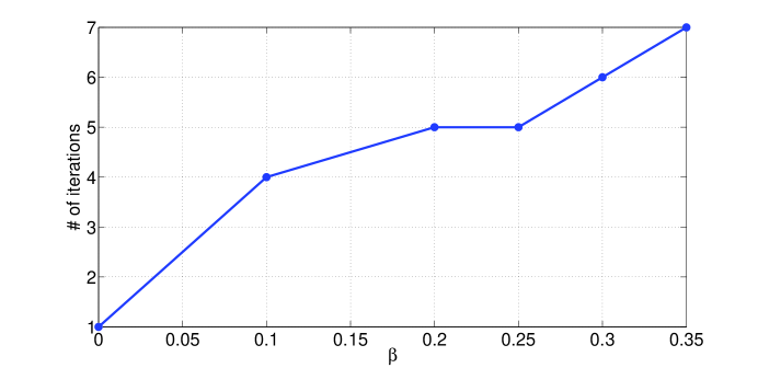
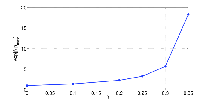
Figure 8. Five-spot problem using $400$ four-node quadrilateral elements: The top figure shows the number of Newton-Raphson iterations for various values of $\beta$. The bottom figure shows the variation of $\exp[\beta p_{\mathrm{max}}]$ for various values of $\beta$, where $\exp[\beta p_{\mathrm{max}}]$ denotes the maximum pressure in the computational domain. We have employed Barus’ formula with $\alpha_{0}=1$.

This subsection presents numerical results for a quarter of the five-spot problem, which exhibits elliptic singularities near (injection and production) wells and is widely used as a good model problem to test the robustness of a numerical formulation. Taking into account the quarter symmetry in the five-spot problem, the source and sink strengths at injection and production wells are, respectively, taken as $+1/4$ and $-1/4$. There is no volumetric source/sink (i.e., $\boldsymbol{b}(\boldsymbol{x})=\boldsymbol{0}$). The five-spot problem is pictorially described in Figure 5. The numerically obtained pressure profiles using Darcy’s equation and modified Darcy’s equation with the viscosity given by Barus’ formula are shown in the Figures 6 and 7. Firstly, there are no spurious oscillations in the pressure field even for the modified Darcy’s equation, and the proposed mixed stabilized formulation performed well. Secondly, for this test problem, pressure in the case of the modified Darcy equation exhibits steeper gradients compared to the pressure field based on Darcy’s equation. In Table 1 we have shown that the norm of the residual vector exhibits terminal quadratic convergence, which basically shows that the tangent matrix corresponding to the given residual vector is correctly formulated and calculated. In nonlinear problems, (due to the lack of analytical solutions) the terminal quadratic convergence is considered as a good measure to check the computer implementation of a numerical formulation. In Figure 8 we compared the number of Newton-Raphson iterations for various values of $\beta$ using four-node quadrilateral elements for a relative tolerance of $10^{-12}$. In the same figure we have also shown the variation of $\exp[\beta p_{\mathrm{max}}]$ with respect to $\beta$, where $p_{\mathrm{max}}$ is the maximum pressure in the computational domain. (Note that $p_{\mathrm{max}}$ occurs at the injection well.) As one can see, as $\beta$ increases $\exp[\beta p_{\mathrm{max}}]$ increases drastically, and very steep pressure gradients occur near the injection and production wells. To obtain results for much higher values of $\beta$ one may have to precondition the resulting linear equations at every Newton-Raphson iteration in order to avoid ill-conditioned matrices, and also employ a finer mesh.

Remark 5.

It is well-known that the Newton-Raphson solution procedure will not always exhibit terminal quadratic convergence. For example, if the multiplicity of the desired root is greater than one, the Newton-Raphson solution procedure may not exhibit terminal quadratic convergence. Also, in some cases, the Newton-Raphson procedure may not even converge. For a detailed discussion of the convergence properties of the Newton-Raphson solution procedure see Reference [53].

Table 1. Five-spot problem: Convergence of Newton-Raphson solution procedure for solving modified Darcy’s equation using four-node quadrilateral (Q4) and three-node triangular (T3) elements. We have used Barus’ formula with $\alpha_{0}=1$ and $\beta=0.3$. The test problem is pictorially described in Figure 5. As one can see from the table, the solution procedure exhibits terminal quadratic convergence.

Iteration #	Norm of residual (Q4)	Norm of residual (T3)
0	0.242406260	0.291915904
1	0.082035285	0.086348093
2	0.037068940	0.037721275
3	0.004513442	0.004318753
4	4.1044706e-05	3.4343232e-05
5	1.4244950e-09	7.6123308e-10
6	2.0953922e-15	3.4935047e-15

5.3. $h$-convergence analysis for a two-dimensional problem

Let us consider a bi-unit square $[0,1]\times[0,1]$ as our computational domain. Let us assume that the velocity and pressure are respectively given as

(75) $$v_{x}(x,y)=\sin(\pi x)\cos(\pi y),\quad v_{y}(x,y)=-\cos(\pi x)\sin(\pi y),\quad p(x,y)=1+25xy(x-1)(y-1)$$

We shall assume that $\rho=1$, $\alpha_{0}=1$, and $\beta=2$. Using the above assumed solution, the required body force under the Barus’ formula (1) should be equal to

(76a) $$b_{x}(x,y) =\exp[\beta(1+25xy(x-1)(y-1))]\sin(\pi x)\cos(\pi y)+25(2x-1)y(y-1)$$

(76b) $$b_{y}(x,y) =-\exp[\beta(1+25xy(x-1)(y-1))]\cos(\pi x)\sin(\pi y)+25x(x-1)(2y-1)$$

and the boundary conditions are given by

(77) $$v_{x}(x=0,y)=v_{x}(x=1,y)=0,\quad v_{y}(x,y=0)=v_{y}(x,y=1)=0$$

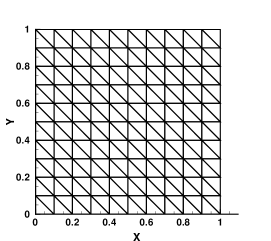
Figure 9. Typical meshes used in the $h$-convergence analysis: (a) four-node quadrilateral (b) three-node triangular (right) meshes.

Using the aforementioned boundary value problem, we shall perform numerical convergence studies of the proposed stabilized mixed formulation for both four-node quadrilateral and three-node triangular elements. Typical uniform finite element meshes used in the $h$-convergence analysis are shown in Figure 9. Note that all the elements in the four-node quadrilateral mesh are squares, and all the elements in the three-node triangular mesh are isosceles right-angled triangles. In the numerical convergence studies presented in this subsection, we have taken $h$ to be equal to the length of the side for square elements, and length of the base (or height) for the isosceles right-angled triangles.

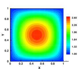
(b) Using three-node triangular elements

Figure 10. Structured meshes: contours of pressure using $100$ uniform four-node quadrilateral (left) and $200$ three-node triangular (right) elements. There are no spurious oscillations in the pressure field.

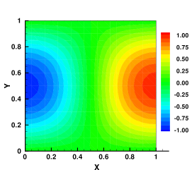
(d) $y$-velocity using T3 elements

Figure 11. Structured meshes: contours of $x$-velocity (top) and $y$-velocity (bottom) using $100$ uniform four-node quadrilateral (Q4) elements and $200$ three-node triangular (T3) elements.

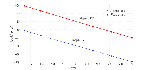
(a) Convergence for four-node quadrilateral elements

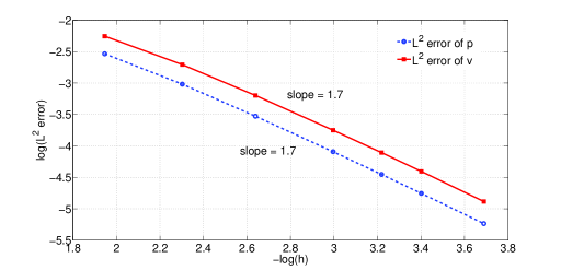
(b) Convergence for three-node triangular elements

Figure 12. 2D $h$-convergence analysis: Rate of convergence of pressure and velocity in the $L^{2}(\Omega)$ norm for four-node quadrilateral and three-node triangular finite elements.

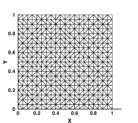
(a) Computational mesh

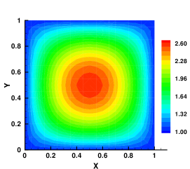
(b) Pressure contours

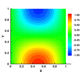
(c) $x$-velocity contours

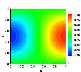
(d) $y$-velocity contours

Figure 13. Unstructured three-node triangular mesh: mesh (top-left), pressure (top-right), $x$-velocity (bottom-left) and $y$-velocity (bottom-right). Barus’ formula is employed with $\alpha_{0}=1$ and $\beta=2$.

The contours of pressure and velocity are shown in Figures 10 and 11. The rates of $h$-convergence of these finite elements for the aforementioned problem are shown in Figure 12. (We have used the natural logarithm in these figures.) For the chosen problem, the proposed formulation converges in both pressure and velocity with respect to $h$-refinement. The above problem (76) is also solved using an unstructured triangular mesh. The obtained numerical results and mesh are shown in Figure 13, quadratic convergence of the Newton-Raphson solution procedure for this problem is illustrated in Table 2, and the proposed mixed stabilized formulation performed well.

Table 2. Unstructured three-node triangular mesh: Convergence of Newton-Raphson solution procedure for solving modified Darcy’s equation. We have used Barus’ formula with $\alpha_{0}=1$ and $\beta=2$. As one can see from the table, the solution procedure exhibits terminal quadratic convergence.

Iteration #	Norm of residual
0	1.353515824
1	3.594631185
2	1.781220654
3	31.25838881
4	0.169839581
5	0.015076303
6	3.125925098e-05
7	7.498072058e-10
8	6.532312307e-16

5.4. A typical reservoir simulation

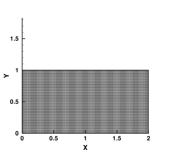
Figure 15. A four-node quadrilateral (structured) finite element mesh used in the reservoir simulation. There are $8000$ elements, $8241$ nodes, and each node has three degrees-of-freedom ($x$- and $y$-velocities, and pressure).

Figure 1 shows how enhanced oil recovery is achieved in the field. A corresponding computational idealization of enhanced oil recovery is shown in Figure 14, which will be discretized using finite elements. The computational mesh is shown in Figure 15. It should be noted that the corner points at the production well are reentrant corners, and hence the velocity $\boldsymbol{v}$ (which is proportional to gradient of pressure) is infinity at those reentrant corner points. We now compare the solutions obtained using Darcy’s equation (constant drag function) and modified Darcy’s equation using Barus’ formula.

For this problem, we have taken $\bar{\alpha}_{0}=1$, $\bar{\beta}=0.005$, $P=1\;\mathrm{atm}$, $B=9.81\;\mathrm{m/s^{2}}$, $\bar{\boldsymbol{b}}=[0,-1]^{T}$, $\mathcal{A}=1$ and $\mathcal{C}=1$. The top surface at the production well is at atmospheric pressure (see Figure 14), which is given by the non-dimensional parameter $\bar{p}_{\mathrm{atm}}=1$ (as we have taken the reference pressure to be $P=1\;\mathrm{atm}$).

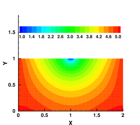
Figure 16. Pressure contours using Darcy’s equation (top) and modified Darcy’s equation (bottom) for $\bar{p}_{\mathrm{enh}}=5$.

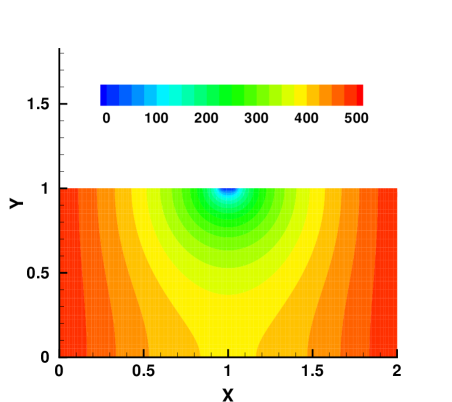
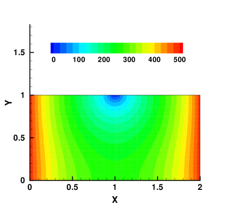
Figure 17. Pressure contours using Darcy’s equation (top) and modified Darcy’s equation (bottom) for $\bar{p}_{\mathrm{enh}}=500$.

In Figures 16 and 17, pressure contours are shown for the cases $\bar{p}_{\mathrm{enh}}=5$ and $\bar{p}_{\mathrm{enh}}=500$, respectively. For low prescribed pressures at the injection wells, the pressure profiles obtained using Darcy’s equation and modified Darcy’s equation are similar. However, this is not the case for higher pressures at the injection wells, and the pressure profiles using Darcy’s and modified Darcy’s equations are significantly different. The pressure using modified Darcy’s equation exhibit steeper gradients near the injection wells. It should be noted that pressure gradients play an important role in the study of fracture of porous medium.

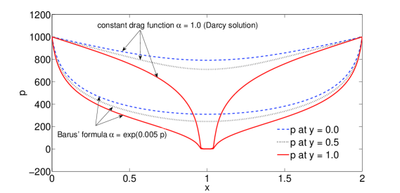
Figure 18. Variation of pressure with respect to horizontal distance from the production well at various depths of the reservoir using Darcy’s equation and modified Darcy’s equation for $\bar{p}_{\mathrm{enh}}=1000$.

In Figure 18, the variations of pressure with respect to the horizontal distance from the production well at various depths are plotted for Darcy’s and modified Darcy’s equations. In this study we have taken $\bar{p}_{\mathrm{enh}}=1000$. As one can see from Figure 18, the pressures from Darcy’s equation and modified Darcy’s equation are qualitatively and quantitatively different. Most importantly, the cone shapes are completely different. (Cone shape is the variation of pressure with respect to the horizontal distance from the production well, and is considered an important parameter in assessing the well performance and also regulating reservoir-operating conditions.) For the case of Darcy’s equation, the graph is concave upwards, while the graph using modified Darcy’s equation (with Barus’ formula) is convex upwards.

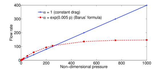
Figure 19. Total flow rate at the production well using Darcy’s equation and modified Darcy’s equation (using Barus’ formula) for various values of $\bar{p}_{\mathrm{enh}}$.

In Figure 19 we compared the total flux at the production well for various pressures at the injection wells (which is given by $\bar{p}_{\mathrm{enh}}$) using Darcy’s equation and modified Darcy’s equation (based on Barus’ formula). Even for this case the pressure at the production well is $\bar{p}_{\mathrm{atm}}=1$. The total flux at the production well is calculated using

(78) $$\int_{\Gamma^{\mathrm{D}}_{1}}\boldsymbol{v}\cdot\boldsymbol{n}\;\mathrm{d}\Gamma$$

where the part of boundary $\Gamma^{\mathrm{D}}_{1}$ is indicated in Figure 14. As one can see in Figure 19, modified Darcy’s equation predicts a ceiling for the total flux with respect to pressure, which is what is expected physically. On the other hand, Darcy’s equation predicts continued linear increase of the total flux with respect to the pressure.

One can expect even more interesting departures from the classical results when the Darcy-Forchheimer and Darcy-Forchheimer-Brinkman equations are modified to incorporate the effect of pressure on the viscosity and drag function. Studying the interactions between the solid deformation and fluid flow, with the effects due to the pressure being taken into account will provide even more insights into the real problem, and is part of our future work.

6. CONCLUSIONS

In this paper we have studied the flow of an incompressible fluid through a rigid porous solid under high pressure and pressure gradients. For such problems, Darcy’s equation is not a good model as it assumes constant viscosity and drag coefficient, which is contrary to experimental evidence. Here, we have considered a modification to Darcy’s equation wherein the drag coefficient is a function of pressure, which is the case with many liquids for large range of pressures. We have allowed the drag coefficient to vary with pressure in different ways, which are primarily motivated by experimental observations. We have also presented a new stabilized mixed formulation for the modified Darcy’s equation along with the incompressibility constraint. The proposed formulation allows equal-order interpolation for pressure and velocity, which is not stable under the classical mixed formulation. A noteworthy feature of the formulation is that the stabilization parameter neither involves mesh-dependent nor material parameters. We have presented representative numerical results to show that the proposed formulation performs well. We have also shown that the solution (both velocity and pressure fields) based on the modified Darcy’s equation is significantly different from the solution based on Darcy’s equation. In particular, using a representative reservoir simulation, we have shown that the Darcy’s model may predict significantly higher flow rate at high pressure as it does not account for variation of viscosity with respect to pressure.

7. APPENDIX

7.1. Notation and definitions

We now define some quantities that will be useful in writing the finite element residual vector and tangent stiffness matrix in a compact manner. Let $\boldsymbol{A}$ and $\boldsymbol{B}$ be matrices of size $n\times m$ and $p\times q$, respectively. That is,

$$\boldsymbol{A}=\left[\begin{array}[]{ccc}a_{1,1}&\ldots&a_{1,m}\\ \vdots&\ddots&\vdots\\ a_{n,1}&\ldots&a_{n,m}\end{array}\right]\ ;\ \boldsymbol{B}=\left[\begin{array}[]{ccc}b_{1,1}&\ldots&b_{1,q}\\ \vdots&\ddots&\vdots\\ b_{p,1}&\ldots&b_{p,q}\end{array}\right]$$

The Kronecker product of these matrices is an $np\times mq$ matrix, and is defined as

$$\boldsymbol{A}\odot\boldsymbol{B}:=\left[\begin{array}[]{ccc}a_{1,1}\boldsymbol{B}&\ldots&a_{1,m}\boldsymbol{B}\\ \vdots&\ddots&\vdots\\ a_{n,1}\boldsymbol{B}&\ldots&a_{n,m}\boldsymbol{B}\end{array}\right]$$

Note that the Kronecker product can defined for any two given matrices (irrespective of their dimensions). The $\mathrm{vec}[\cdot]$ operator is defined as

$$\mathrm{vec}[\boldsymbol{A}]:=\left[\begin{array}[]{c}a_{1,1}\\ \vdots\\ a_{1,m}\\ \vdots\\ a_{n,1}\\ \vdots\\ a_{n,m}\end{array}\right]$$

Some relevant properties of Kronecker product and $\mathrm{vec}[\cdot]$ operator are as follows:

• $\mathrm{vec}[\boldsymbol{ACB}]=\left(\boldsymbol{B}^{T}\odot\boldsymbol{A}\right)\mathrm{vec}[\boldsymbol{C}]$

• $\left(\boldsymbol{A}\odot\boldsymbol{B}\right)\left(\boldsymbol{C}\odot\boldsymbol{D}\right)=\left(\boldsymbol{A}\boldsymbol{C}\odot\boldsymbol{B}\boldsymbol{D}\right)$

• $\mathrm{vec}[\boldsymbol{A}+\boldsymbol{B}]=\mathrm{vec}[\boldsymbol{A}]+\mathrm{vec}[\boldsymbol{B}]$

For a detailed discussion on Kronecker products and $\mathrm{vec}[\cdot]$ operator see References [51, 54, 55].

Figure 2. Typical two-dimensional finite elements employed in the numerical simulations, and the location of velocity and pressure unknowns. Equal-order interpolation is used for the velocity and pressure.

\psfrag{p1}{$\bar{p}(0)=\bar{p}_{1}$}\psfrag{p2}{$\bar{p}(1)=\bar{p}_{2}$}\psfrag{x}{$\bar{x}$}\psfrag{1.0}{$1.0$}\includegraphics[scale={0.75}]{Figures/OneD_problem.eps}

Figure 3. Schematic description of the one-dimensional problem.

\psfrag{p}{$\bar{p}$}\psfrag{x}{$\bar{x}$}\includegraphics[scale={0.3}]{Figures/OneD_problem_P1_200_P2_1.eps}

Figure 4. One-dimensional problem: The numerically obtained pressure profiles are compared against analytical solutions for various drag functions. We have chosen $\bar{p}_{1}=200$, $\bar{p}_{2}=1$, $\mathcal{A}=1$, and $\bar{\alpha}_{0}=1$. The body force is neglected. The test problem is pictorially described in Figure 3, and the analytical solutions are given in equation (74).

\psfrag{vx}{$v_{x}=0$}\psfrag{vy}{$v_{y}=0$}\includegraphics[scale={0.75}]{Figures/Five_spot_description.eps}

Figure 5. Pictorial description of a quarter of five-spot problem.

(a) Using four-node quadrilateral elements

(a) $x$-velocity using Q4 elements

(b) $x$-velocity using T3 elements

(c) $y$-velocity using Q4 elements

\psfrag{vn}{$\boldsymbol{v}\cdot\boldsymbol{n}=0$}\psfrag{g}{$\Gamma^{\mathrm{N}}$}\psfrag{D1}{$\Gamma^{\mathrm{D}}_{1}$}\psfrag{D2}{$\Gamma^{\mathrm{D}}_{2}$}\psfrag{p1}{$p(\boldsymbol{x})=p_{\mathrm{atm}}$}\psfrag{p2}{$p(\boldsymbol{x})=p_{\mathrm{enh}}$}\includegraphics[scale={0.5}]{Figures/Computational_well.eps}

Figure 14. Top figure is a pictorial description of a reservoir. Water, steam or Carbon dioxide is pumped through injection wells, and crude oil is collected at the production well. Bottom figure shows the computational idealization of the reservoir with appropriate boundary conditions. On $\Gamma^{\mathrm{D}}_{1}$ we prescribe $p(\boldsymbol{x})=p_{\mathrm{atm}}$, and on $\Gamma^{\mathrm{D}}_{2}$ we prescribe $p(\boldsymbol{x})=p_{\mathrm{enh}}$.

References

- [1] H. Darcy. Les Fontaines Publiques de la Ville de Dijon. Victor Dalmont, Paris, 1856.
- [2] G. G. Stokes. On the theories of internal friction of fluids in motion and of the equilibrium and motion of elastic solids. Transactions of Cambridge Philosophical Society, 8:287–305, 1845.
- [3] C. Barus. Isotherms, isopiestics and isometrics relative to viscosity. American Journal of Science, 45:87–96, 1893.
- [4] P. W. Bridgman. The Physics of High Pressure. MacMillan Company, New York, USA, 1931.
- [5] E. Höglund. Influence of lubricant properties on elastohydrodynamic lubrication. Wear, 232:176–184, 1999.
- [6] D. Dowson and G. R. Higginson. Elastohydrodynamic Lubrication: The Fundamentals of Roller and Gear Lubrication. Pergamon Press, 1966.
- [7] Z. Chen, G. Huan, and Y. Ma. Computational Methods for Multiphase Flows in Porous Media. Society for Industrial and Applied Mathematics, Philadelphia, USA, 2006.
- [8] A. Masud and T. J. R. Hughes. A stabilized mixed finite element method for Darcy flow. Computer Methods in Applied Mechanics and Engineering, 191:4341–4370, 2002.
- [9] R. E. Ewing and R. F. Heinemann. Convergence analysis of an approximation of miscible displacement in porous media by mixed finite elements and a modified method of characteristics. Computer Methods in Applied Mechanics and Engineering, 47:73–92, 1984.
- [10] G. Chavent, G. Cohen, and J. Jaffre. Discontinuous upwinding and mixed finite element for two-phase flows in reservoir simulation. Computer Methods in Applied Mechanics and Engineering, 47:93–118, 1984.
- [11] R. E. Ewing and R. F. Heinemann. Mixed finite element approximation of phase velocities in compositional reservoir simulation. Computer Methods in Applied Mechanics and Engineering, 47:161–175, 1984.
- [12] L. J. Durlofsky. Accuracy of mixed and control volume finite element approximations to Darcy velocity and related quantities. Water Resources Research, 30:965–973, 1994.
- [13] T. Arbogast, M. F. Wheeler, and I. Yotov. Mixed finite elements for elliptic problems with tensor coefficients as cell-centered finite differences. SIAM Journal on Numerical Analysis, 34:828–852, 1997.
- [14] L. Bergamaschi, S. Mantica, and G. Manzini. A mixed finite element-volume formulation of the black oil model. SIAM Journal of Scientific Computing, 20:970–997, 1998.
- [15] F. Brezzi, T. J. R. Hughes, L. D. Marini, and A. Masud. Mixed discontinuous Galerkin method for Darcy flow. SIAM Journal of Scientific Computing, 22:119–145, 2005.
- [16] T. J. R. Hughes, A. Masud, and J. Wan. A stabilized mixed discontinuous Galerkin method for Darcy flow. Computer Methods in Applied Mechanics and Engineering, 195:3347–3381, 2006.
- [17] K. B. Nakshatrala, D. Z. Turner, K. D. Hjelmstad, and A. Masud. A stabilized mixed finite element formulation for Darcy flow based on a multiscale decomposition of the solution. Computer Methods in Applied Mechanics and Engineering, 195:4036–4049, 2006.
- [18] E. Burman and P. Hansbo. A unified stabilized method for Stokes’ and Darcy’s equations. Journal of Computational and Applied Mathematics, 198:35–51, 2007.
- [19] I. Babuška. Error bounds for finite element methods. Numerische Mathematik, 16:322–333, 1971.
- [20] F. Brezzi and M. Fortin. Mixed and Hybrid Finite Element Methods, volume 15 of Springer series in computational mathematics. Springer-Verlag, New York, USA, 1991.
- [21] I. Babuška, J. T. Oden, and J. K. Lee. Mixed-hybrid finite element approximations of second-order elliptic boundary-value problems. Computer Methods in Applied Mechanics and Engineering, 11:175–206, 1977.
- [22] A. N. Brooks and T. J. R. Hughes. Streamline-upwind/Petrov-Galerkin methods for convection dominated flows with emphasis on the incompressible Navier-Stokes equations. Computer Methods in Applied Mechanics and Engineering, 32:199–259, 1982.
- [23] J. T. Oden and O.-P. Jacquotte. Stability of some mixed finite element methods for Stokesian flows. Computer Methods in Applied Mechanics and Engineering, 43:231–247, 1984.
- [24] T. J. R. Hughes, L. Franca, and M. Balestra. A new finite element formulation for computational fluid dynamics: V. Circumventing the Babuska-Brezzi condition: A stable Petrov-Galerkin formulation of the Stokes problem accommodating equal-order interpolations. Computer Methods in Applied Mechanics and Engineering, 59:85–99, 1986.
- [25] L. P. Franca and T. J. R. Hughes. Two classes of mixed finite element methods. Computer Methods in Applied Mechanics and Engineering, 69:89–129, 1988.
- [26] J. Doughlas and J. Wang. An absolutely stabilized finite element method for the Stokes problem. Mathematics of Computation, 52:495–508, 1989.
- [27] T. J. R. Hughes, L. Franca, and G. Hulbert. A new finite element formulation for computational fluid dynamics: VIII. The Galerkin/least-squares method for advective-diffusive equations. Computer Methods in Applied Mechanics and Engineering, 73:173–189, 1989.
- [28] L. P. Franca, S. L. Frey, and T. J. R. Hughes. Stabilized finite element methods: I. Application to the advective-diffusive model. Computer Methods in Applied Mechanics and Engineering, 95:253–276, 1992.
- [29] L. P. Franca and A. Russo. Unlocking with residual-free bubbles. Computer Methods in Applied Mechanics and Engineering, 142:361–364, 1997.
- [30] E. Burman and P. Hansbo. Stabilized Crouzeix-Raviart Elements for the Darcy-Stokes Problem. Numerical Methods for Partial Differential Equations, 21:986–997, 2005.
- [31] M. R. Correa and A. F. D. Loula. Unconditionally stable mixed finite element methods for Darcy flow. Computer Methods in Applied Mechanics and Engineering, 197:1525–1540, 2008.
- [32] A. Quarternio and A. Valli. Numerical Approximation of Partial Differential Equations. Springer series in computational mathematics. Springer-Verlag, New York, USA, 1997.
- [33] H.-G. Roos, M. Stynes, and L. Tobiska. Numerical Methods for Singularly Perturbed Differential Equations. Springer-Verlag, New York, USA, 1996.
- [34] R. J. Atkin and R. E. Craine. Continuum theories of mixtures: Basic theory and historical development. The Quaterly Journal of Mechanics and Applied Mathematics, 29:209–244, 1976.
- [35] R. M. Bowen. Theory of mixtures. In A. C. Eringen, editor, Continuum Physics, volume III. Academic Press, New York, 1976.
- [36] A. Bedford and D. S. Drumheller. Theories of immiscible and structured mixtures. International Journal of Engineering Science, 21:863–960, 1983.
- [37] K. R. Rajagopal and L. Tao. Mechanics of Mixtures. World Scientific Publishing, River Edge, New Jersey, USA, 1995.
- [38] K. R. Rajagopal. On a hierarchy of approximate models for flows of incompressible fluids through porous solids. Mathematical Models and Methods in Applied Sciences, 17:215–252, 2007.
- [39] P. Forchheimer. Wasserbewegung durch Boden. Zeitschrift des Vereines Deutscher Ingeneieure, 45:1782–1788, 1901.
- [40] J. Málek, J. Nečas, and K. R. Rajagopal. Global analysis of the flows of fluids with pressure-dependent viscosities. Archive for Rational Mechanics and Analysis, 165:243–269, 2002.
- [41] J. Hron, J. Málek, J. Nečas, and K. R. Rajagopal. Numerical simulations and global existence of solutions of two-dimensional flows of fluids with pressure-and shear-dependent viscosities. Mathematics and Computers in Simulation, 61:297–315, 2003.
- [42] M. Franta, J. Málek, and K. R. Rajagopal. On steady flows of fluids with pressure- and shear-dependent viscosities. Proceedings of Royal Society A: Mathematical, Physical and Engineering Sciences, 461:651–670, 2005.
- [43] M. Buliček, J. Málek, and K. R. Rajagopal. Navier’s slip and evolutionary Navier-Stokes-like systems with pressure and shear-rate depedent viscosity. Indiana University Mathematics Journal, 56:51–85, 2007.
- [44] M. D. Gunzburger. Finite Element Methods for Viscous Incompressible Flows. Academic Press, San Diego, USA, 1989.
- [45] P. A. Raviart and J. M. Thomas. A mixed finite element method for 2nd order elliptic problems. In Mathematical Aspects of the Finite Element Method, pages 292–315, Springer-Verlag, New York, 1977.
- [46] J. C. Nedelec. Mixed finite elements in . Numerische Mathematik, 35:315–341, 1980.
- [47] J. C. Nedelec. A new family of mixed finite elements in . Numerische Mathematik, 50:57–81, 1986.
- [48] F. Brezzi, J. Douglas, and L. D. Marini. Two families of mixed elements for second order elliptic problems. Numerische Mathematik, 47:217–235, 1985.
- [49] F. Brezzi, J. Douglas, R. Durran, and L. D. Marini. Mixed finite elements for second order elliptic problems in three variables. Numerische Mathematik, 51:237–250, 1987.
- [50] F. Brezzi, J. Douglas, M. Fortin, and L. D. Marini. Efficient rectangular mixed finite elements in two and three space variables. Mathematical Modelling and Numerical Analysis, 21:581–604, 1987.
- [51] A. Graham. Kronecker Products and Matrix Calculus: With Applications. Halsted Press, Chichester, UK, 1981.
- [52] O. C. Zienkiewicz and R. L. Taylor. The Finite Element Method : Vol.1. McGraw-Hill, New York, USA, 1989.
- [53] C. T. Kelley. Solving Nonlinear Equations with Newton’s Method. Society for Industrial and Applied Mathematics, Philadelphia, USA, 1987.
- [54] A. L. Laub. Matrix Analysis for Scientists and Engineers. SIAM, Philadelphia, USA, 7 edition, 2004.
- [55] D. W. Nicholson. Finite Element Analysis: Thermomechanics of Solids. CRC Press, Boca Raton, Florida, USA, 2003.