A Discussion on Mean Excess Plots

Abstract.

A widely used tool in the study of risk, insurance and extreme values is the mean excess plot. One use is for validating a generalized Pareto model for the excess distribution. This paper investigates some theoretical and practical aspects of the use of the mean excess plot.

1. Introduction

The distribution of the excess over a threshold $u$ for a random variable $X$ with distribution function $F$ is defined as

(1.1) $$F_{u}(x)=P\big{[}X-u\leq x|X>u\big{]}.$$

This excess distribution is the foundation for peaks over threshold (POT) modeling (Embrechts et al., 1997; Coles, 2001) which fits appropriate distributions to data of excesses. The use of peaks over threshold modeling is widespread and applications include:

• Hydrology: It is critical to model the level of water in a river or sea to avoid flooding. The level $u$ could represent the height of a dam, levee or river bank. See Todorovic and Zelenhasic (1970) and Todorovic and Rousselle (1971).

• Actuarial science: Insurance companies set premium levels based on models for large losses. Excess of loss insurance pays for losses exceeding a contractually agreed amount. See Hogg and Klugman (1984), Embrechts et al. (2005).

• Survival analysis: The POT method is used for modeling lifetimes; see Guess and Proschan (1985).

• Environmental science: Public health agencies set standards for pollution levels. Exceedances of these standards generate public alerts or corrective measures; see Smith (1989).

Peaks over threshold modeling is based on the generalized Pareto class of distributions being appropriate for describing statistical properties of excesses. A random variable $X$ has a generalized Pareto distribution (GPD) if it has a cumulative distribution function of the form

(1.2) $$G_{\xi,\beta}(x)=\left\{\begin{array}[]{ll}1-(1+\xi x/\beta)^{-1/\xi}&\mbox{ if }\xi\neq 0\\ 1-\exp(-x/\beta)&\mbox{ if }\xi=0\end{array}\right.$$

where $\beta>0$, and $x\geq 0$ when $\xi\geq 0$ and $0\leq x\leq-\beta/\xi$ if $\xi<0$. The parameters $\xi$ and $\beta$ are referred to as the shape and scale parameters respectively. For a Pareto distribution, the tail index $\alpha$ is just the reciprocal of $\xi$ when $\xi>0$. A special case is when $\xi=0$ and in this case the GPD is the same as the exponential distribution with mean $\beta$.

The Pickands-Balkema-de Haan Theorem (Embrechts et al., 2005, Theorem 7.20, page 277) provides the theoretical justification for the centrality of the GPD class of distributions for peaks over threshold modeling. This result shows that for a large class of distributions (those distributions in a maximal domain of attraction of the extreme value laws), the excess distribution $F_{u}$ is asymptotically equivalent to a GPD law $G_{\xi,\beta(u)}$, as the threshold $u$ appropaches the right endpoint of the distribution $F$. Here the asymptotic shape parameter $\xi$ is fixed but the scale $\beta(u)$ may depend on $u$. More precise statements are given below in Theorems 3.1, 3.6, and 3.9. For this reason the GPD is a natural candidate for modeling peaks over a threshold.

The choice of the extreme threshold $u$, where the GPD model provides a suitable approximation to the excess distribution $F_{u}$ is critical in applications. The mean excess (ME) function is a popular tool used to aide this choice of $u$ and also to determine the adequacy of the GPD model in practice. The ME function of a random variable $X$ is defined as:

(1.3) $$M(u):=E\big{[}X-u|X>u\big{]},$$

provided $EX_{+}<\infty,$ and is also known as the mean residual life function, especially in survival analysis. It has been studied as early as Benktander and Segerdahl (1960). See Hall and Wellner (1981) for a discussion of properties of mean excess functions. Table 3.4.7 in (Embrechts et al., 1997, p.161) gives the mean excess function for some standard distributions.

Given an independent and identically distributed (iid) sample $X_{1},\dots,X_{n}$ from $F(x)$, a natural estimate of $M(u)$ is the empirical ME function $\hat{M}(u)$ defined as

(1.4) $$\hat{M}(u)=\frac{\sum_{i=1}^{n}(X_{i}-u)I_{[X_{i}>u]}}{\sum_{i=1}^{n}I_{[X_{i}>u]}},\ \ \ \ u\geq 0.$$

Yang (1978) suggested the use of the empirical ME function and established the uniform strong consistency of $\hat{M}(u)$ over compact $u$-sets; that is, for any $b>0$

(1.5) $$P\Big{[}\lim_{n\to\infty}\sup_{0\leq u\leq b}\big{|}\hat{M}(u)-M(u)\big{|}=0\Big{]}=1.$$

In the context of extremes, however, (1.5) is not especially informative since what is of interest is the behavior of $\hat{M}(u)$ in a neighborhood of the right end point of $F$, which could be $\infty$. In this case the GPD plays a pivotal role. For a random variable $X\sim G_{\xi,\beta}$ , we have $E(X)<\infty$ iff $\xi<1$ and in this case, the ME function of $X$ is linear in $u$:

(1.6) $$M(u)=\frac{\beta}{1-\xi}+\frac{\xi}{1-\xi}u,$$

where $0\leq u<\infty$ if $0\leq\xi<1$ and $0\leq u\leq-\beta/\xi$ if $\xi<0$. In fact, the linearity of the mean excess function characterizes the GPD class. See Embrechts et al. (2005, 1997). Davison and Smith (1990) used this property to devise a simple graphical check that data conforms to a GPD model; their method is based on the ME plot which is the plot of the points $\{(X_{(k)},\hat{M}(X_{(k)})):1<k\leq n\}$, where $X_{(1)}\geq X_{(2)}\geq\cdots\geq X_{(n)}$ are the order statistics of the data. If the ME plot is close to linear for high values of the threshold then there is no evidence against use of a GPD model. See also Embrechts et al. (1997) and Hogg and Klugman (1984) for the implementation of this plot in practice.

In this paper we establish the asymptotic behavior of the ME plots for large thresholds. We assume $F$ is in the maximal domain of attraction of an extreme value law with shape parameter $\xi$. When $\xi<1,$ we show that, as expected, for high thresholds the ME plot viewed as a random closed set converges in the Fell topology to a straight line. A novel aspect of our study is we also consider the ME plot in the case $\xi>1$, the case where the ME function does not exist, and show that the ME plot converges to a random curve. This also holds in the more delicate case $\xi=1$ after suitable rescaling. These results show that the ME plot is inconsistent when $\xi\geq 1$ and emphasizes that knowledge of a finite mean is required.

It is tempting to argue that consistency of the ME plot $\hat{M}(u)$ should imply, by a continuity argument, the consistency of the estimator of $\xi$ obtained from computing the slope of the line fit to the ME plot. However, this slope functional is not necessarily continuous as discussed in Das and Resnick (2008). So consistency of the slope function requires further work and is an ongoing investigation.

The paper is arranged as follows. In Section 2 we briefly discuss required background on convergence of random closed sets and then study the ME plot in Section 3. In Section 4 we discuss advantages and disadvantages of the mean excess plot and how this tool compares with other techniques of extreme value theory such as the Hill estimator, the Pickands estimator and the QQ plot. We illustrate the behavior of the empirical mean excess plot for some simulated data sets in Section 5 and in Section 6 we analyze three real data sets obtained from different subject areas and also compare different tools.

2. Background

2.1. Topology on closed sets of $\mathbb{R}^{2}$

Before we start any discussion on whether a mean excess plot is a reasonable diagnostic tool we need to understand what it means to talk about convergence of plots. So we discuss the topology on a set containing the plots.

We denote the collection of closed subsets of $\mathbb{R}^{2}$ by $\mathcal{F}$. We consider a hit and miss topology on $\mathcal{F}$ called the Fell topology. The Fell topology is generated by the families$\{\mathcal{F}^{K},K\mbox{ compact}\}$ and $\{\mathcal{F}_{G},G\mbox{ open}\}$ where for any set $B$

$$\mathcal{F}^{B}=\{F\in\mathcal{F}:F\cap B=\emptyset\}\ \ \mbox{ and }\ \ \mathcal{F}_{B}=\{F\in\mathcal{F}:F\cap B\neq\emptyset\}$$

So $\mathcal{F}^{B}$ and $\mathcal{F}_{B}$ are collections of closed sets which miss and hit the set $B$, respectively. This is why such topologies are called hit and miss topologies. In the Fell topology a sequence of closed sets $\{F_{n}\}$ converges to $F\in\mathcal{F}$ if and only if the following two conditions hold:

• $F$ hits an open set $G$ implies there exists $N\geq 1$ such that for all $n\geq N$, $F_{n}$ hits $G$.

• $F$ misses a compact set $K$ implies there exists $N\geq 1$ such that for all $n\geq N$, $F_{n}$ misses $K$.

The Fell topology on the closed sets of $\mathbb{R}^{2}$ is metrizable and we indicate convergence in this topology of a sequence $\{F_{n}\}$ of closed sets to a limit closed set $F$ by $F_{n}\to F$. Sometimes, rather than work with the topology, it is easier to deal with the following characterization of convergence.

Lemma 2.1.

A sequence $F_{n}\in\mathcal{F}$ converges to $F\in\mathcal{F}$ in the Fell topology if and only if the following two conditions hold:

1. For any $t\in F$ there exists $t_{n}\in F_{n}$ such that $t_{n}\to t.$

2. If for some subsequence $(m_{n})$, $t_{m_{n}}\in F_{m_{n}}$ converges, then $\lim\limits_{n\to\infty}t_{m_{n}}\in F$.

See Theorem 1-2-2 in (Matheron, 1975, p.6) for a proof of this Lemma. Since the topology is metrizable, the definition of convergence in probability is obvious. The following result is a well-known and helpful characterization for convergence in probability of random variables and it holds for random sets as well; see Theorem 6.21 in (Molchanov, 2005, p.92).

Lemma 2.2.

A sequence of random sets $(F_{n})$ in $\mathcal{F}$ converges in probability to a random set $F$ if and only if for every subsequence $(n^{\prime})$ of $\mathbb{Z}_{+}$ there exists a further subsequence $(n^{\prime\prime})$ of $(n^{\prime})$ such that $F_{n^{\prime\prime}}\to F$-a.s.

We use the following notation: For a real number $x$ and a set $A\subset\mathbb{R}^{n}$, $xA=\{xy:y\in A\}$.

Matheron (1975) and Molchanov (2005) are good references for the theory of random sets.

2.2. Miscellany.

Throughout this paper we will take $k:=k_{n}$ to be a sequence increasing to infinity such that $k_{n}/n\to 0$. For a distribution function $F(x)$ we write $\bar{F}(x)=1-F(x)$ for the tail and the quantile function is

$$F^{\leftarrow}(1-\frac{1}{u})=\inf\{s:F(s)\geq 1-\frac{1}{u}\}=\Bigl{(}\frac{1}{1-F}\Bigr{)}^{\leftarrow}(u).$$

A function $U:(0,\infty)\mapsto\mathbb{R}_{+}$ is regularly varying with index $\rho\in\mathbb{R}$, written $U\in RV_{\rho}$, if

$$\lim_{t\to\infty}\frac{U(tx)}{U(t)}=x^{\rho},\quad x>0.$$

We denote the space of nonnegative Radon measures $\mu$ on $(0,\infty]$ metrized by the vague metric by $M_{+}(0,\infty]$. Point measures are written as a function of their points $\{x_{i},i=1,\dots,n\}$ by $\sum_{i=1}^{n}\delta_{x_{i}}.$ See, for example, (Resnick, 1987, Chapter 3).

We will use the following notations to denote different classes of functions: For $0\leq a<b\leq\infty$

1. $D[a,b)$: Right-continuous functions with finite left limits defined on $[a,b)$.

2. $D_{l}[a,b)$: Left-continuous functions with finite right limits defined on $[a,b)$.

We will assume that these spaces are equipped with the Skorokhod topology and the distance function. In some cases we will also consider product spaces of functions and then the topology will be the product topology. For example, $D^{2}_{l}[1,\infty)$ will denote the class of 2-dimensional functions on $[1,\infty)$. The classes of functions defined on the sets $[a,b]$ or $(a,b]$ will have the obvious notation.

3. Mean Excess Plots

As discussed in the introduction, a random variable having $G_{\xi,\beta}$ distribution with $\xi<1$ has a linear ME function given by (1.6) where the slope $\xi$ is positive $(0<\xi<1),$ negative or $\xi=0$. We consider these three cases separately.

3.1. Positive Slope

In this subsection we concentrate on the case where $\xi>0$. A finite mean for $F$ is guaranteed when $\xi<1$ and we also investigate what happens when $\xi\geq 1$.

The following Theorem is a combination of Theorem 3.3.7 and Theorem 3.4.13(b) in Embrechts et al. (1997).

Theorem 3.1.

Assume $\xi>0$. The following are equivalent for a cumulative distribution function $F$:

1. $\bar{F}\in RV_{-1/\xi}$, i.e., for every $t>0$ $\lim_{x\rightarrow\infty}\frac{\bar{F}(tx)}{\bar{F}(x)}=t^{-1/\xi}.$

2. $F$ is in the maximal domain of attraction of a Frechet distribution with parameter $1/\xi$, i.e.,

   $$\lim_{n\rightarrow\infty}F^{n}(c_{n}x)=\exp\{-x^{-1/\xi}\}\ \ \ \ \mbox{ for all }x>0.$$

   where $c_{n}=F^{\leftarrow}(1-n^{-1})$.

3. There exists a positive measurable function $\beta(u)$ such that

   (3.1) $$\lim_{u\rightarrow\infty}\sup_{x\geq u}\big{|}F_{u}(x)-G_{\xi,\beta(u)}(x)\big{|}=0.$$

Theorem 3.1(3) is one case of the Pickands-Balkema-de Haan theorem. It guarantees the existence of a measurable function $\beta(u)$ for which (3.1) holds but does not construct this function. However, $\beta(u)$ can be obtained from Karamata’s representation of a regular varying function (Bingham et al., 1989), namely if $\bar{F}\in RV_{-1/\xi}$, there exists $0<z<\infty$ such that

$$\bar{F}(x)=c(x)\exp\left\{\int_{z}^{x}\frac{1}{a(t)}dt\right\}\ \ \ \ \mbox{ for all }z<x<\infty$$

where $c(x)\to c>0$ and $a(x)/x\to\xi$ as $x\to\infty$. An easy computation shows as $u\to\infty$,

$$\frac{\bar{F}(u+xa(u))}{\bar{F}(u)}= (1+o(1))\exp\left\{-\int_{u}^{u+xa(u)}\frac{1}{a(t)}dt\right\}$$

$$= (1+o(1))\exp\left\{-\int_{u}^{u+x\xi u(1+o(1))}\frac{t}{a(t)}\frac{dt}{t}\right\}\to(1+\xi x)^{-1/\xi}.$$

This means that if $X$ is a random variable having distribution $F$ then for large $u$,

$$P\Big{[}\frac{X-u}{a(u)}\leq x\Big{|}X>u\Big{]}\approx G_{\xi,1}(x)$$

and $a(u)$ is a choice for the scale parameter $\beta(u)$ in (3.1). Hence we get that $\beta(u)/u\to\xi$ as $u\to\infty$ by the convergence to types theorem (Resnick, 1987).

Consider the ME plot for iid random variables having common distribution $F$ which satisfies $\bar{F}\in RV_{-1/\xi}$ for some $\xi>0$. Since the excess distribution is well approximated by the GPD for high thresholds, we expect that for $\xi<1$, the ME function will look similar to that of the GPD for high thresholds and therefore seek evidence of linearity in the plot. We first consider the ME plot when $0<\xi<1$ and will discuss the case $\xi\geq 1$ separately. Furthermore, we see that for each $n\geq 1$, the mean excess plot, being a finite set of $\mathbb{R}^{2}$-valued random variables, is measurable and a random closed set. It follows from the definition of random sets; see Definition 1.1 in (Molchanov, 2005, p. 2).

3.1.1. Heavy tail with a finite mean; $0<\xi<1$.

The scaled and thresholded ME plot converges to a deterministic line.

Theorem 3.2.

If $(X_{n},n\geq 1)$ are iid observations with distribution $F$ satisfying $\bar{F}\in RV_{-1/\xi}$ with $0<\xi<1$, then in $\mathcal{F}$

(3.2) $$\mathcal{S}_{n}:=\frac{1}{X_{(k)}}\left\{\big{(}X_{(i)},\hat{M}(X_{(i)})\big{)}:i=2,\ldots,k\right\}\stackrel{{\scriptstyle P}}{{\longrightarrow}}\mathcal{S}:=\Big{\{}\Big{(}t,\frac{\xi}{1-\xi}t\Big{)}:t\geq 1\Big{\}}.$$

Remark 3.3.

Roughly, this result implies

$$X_{(k)}\mathcal{S}_{n}:=\left\{\big{(}X_{(i)},\hat{M}(X_{(i)})\big{)}:i=2,\ldots,k_{n}\right\}\approx X_{(k)}\mathcal{S}.$$

The plot of the points $\mathcal{S}_{n}$ is a little different from the original ME plot. In practice, people plot of the points $\{(X_{(i)}),\hat{M}(X_{(i)}):1<i\leq n\}$ but our result restricts attention to the higher order statistics corresponding to $X_{(1)},\dots,X_{(k)}.$ This restriction is natural and corresponds to looking at observations over high thresholds. One imagines zooming into the area of interest in the complete ME plot.

This result scales the points $(X_{(i)},\hat{M}(X_{(i)}))$ by $X_{(k)}^{-1}$. Since both co-ordinates of the points in the plot are scaled, we do not change the structure or appearance of the plot but only the scale of the axes. Hence we may still estimate the slope of the line if we want to estimate $\xi$ by this method (Davison and Smith, 1990). The scaling is important because the points $\{(X_{(i)}),\hat{M}(X_{(i)}):1<i\leq k\}$ are moving to infinity and the Fell topology is not equipped to handle sets which are moving out to infinity. Furthermore, the regular variation assumption on the tail of $F$ involves a ratio condition and thus it is natural that the random set convergence uses scaling.

A central assumption in Theorem 3.2 is that the random variables $\{X_{i}\}$ are iid. The proof of the theorem below will explain that an important tool is the convergence of the tail empirical measure $\hat{\nu}_{n}$ in (3.4). By Proposition 2.1 in Resnick and Starica (1998), we know that the iid assumption of the random variables is not a necessary condition for the convergence of the tail empirical measure. We believe as long as the tail empirical measure converges, our result should hold.

Proof.

We show that for every subsequence $m_{n}$ of integers there exists a further subsequence $l_{n}$ of $m_{n}$ such that

(3.3) $$\mathcal{S}_{l_{n}}\to\mathcal{S}\ \ \ \ \mbox{ a.s. }$$

Define the tail empirical measure as a random element of $M_{+}(0,\infty]$ by

(3.4) $$\hat{\nu}_{n}:=\frac{1}{k}\sum_{i=1}^{n}\delta_{X_{i}/X_{(k)}}.$$

Following (4.21) in (Resnick, 2007, p.83) we get that

(3.5) $$\hat{\nu}_{n}\Rightarrow\nu\ \ \ \ \mbox{ in }M_{+}(0,\infty]$$

where $\nu(x,\infty]=x^{-1/\xi},x>0.$ Now consider

$$S_{n}(u)=\Big{(}\frac{X_{(\lceil ku\rceil)}}{X_{(k)}},\frac{\hat{M}(X_{(\lceil ku\rceil)})}{X_{(k)}}\Big{)}\ \ \ \ u\in(0,1]$$

as random elements in $D^{2}_{l}(0,1]$.We will show that $S_{n}(\cdot)\stackrel{{\scriptstyle P}}{{\longrightarrow}}S(\cdot)$ in $D^{2}_{l}(0,1]$, where

$$S(u)=\Big{(}u^{-\xi},\frac{\xi}{1-\xi}u^{-\xi}\Big{)}\ \ \ \ \mbox{ for all }0<u\leq 1.$$

We already know the result for the first component of $S_{n}$, i.e., $S^{(1)}_{n}(t):=X_{(\lceil kt\rceil)}/X_{(k)}\stackrel{{\scriptstyle P}}{{\to}}t^{-\xi}$ in $D_{l}(0,1]$; see (Resnick, 2007, p.82). Since the limits are non-random it suffices to prove the convergence of the second component of $S_{n}$. Observe that the empirical mean excess function can be obtained from the tail empirical measure:

$$S^{(2)}_{n}(u):=\frac{\hat{M}(X_{(\lceil ku\rceil)})}{X_{(k)}}=\frac{k}{\lceil ku\rceil-1}\int_{X_{(\lceil ku\rceil)}/X_{(k)}}^{\infty}\hat{\nu}_{n}(x,\infty]dx.$$

Consider the maps $T$ and $T_{K}$ from $M_{+}(0,\infty]$ to $D_{l}[1,\infty)$ defined by

$$T(\mu)(t)=\int_{t}^{\infty}\mu(x,\infty]dx\ \ \mbox{ and }\ \ T_{K}(\mu)(t)=\int_{t}^{K\vee t}\mu(x,\infty]dx.$$

We understand $T(\mu)(t)=\infty$ if $\mu(x,\infty]$ is not integrable. We will show that $T(\hat{\nu}_{n})\stackrel{{\scriptstyle P}}{{\to}}T(\nu)$. The function $T_{K}$ is obviously continuous and therefore $T_{K}(\hat{\nu}_{n})\stackrel{{\scriptstyle P}}{{\to}}T_{K}(\nu)$ in $D_{l}[1,\infty)$. In order to prove that $T(\hat{\nu}_{n})\stackrel{{\scriptstyle P}}{{\to}}T(\nu)$ it suffices to show that for any $\epsilon>0$

$$\lim_{K\rightarrow\infty}\limsup_{n\rightarrow\infty}P\Big{[}\big{\|}T_{K}(\hat{\nu}_{n})-T(\hat{\nu}_{n})\big{\|}>\epsilon\Big{]}=0,$$

where $\|\cdot\|$ is the supnorm on $D_{l}[1,\infty)$. To verify this claim, note that

$$\lim_{K\rightarrow\infty}\limsup_{n\rightarrow\infty}P\Big{[}\big{\|}T_{K}(\hat{\nu}_{n})-T(\hat{\nu}_{n})\big{\|}>\epsilon\Big{]}\leq\lim_{K\rightarrow\infty}\limsup_{n\rightarrow\infty}P\Big{[}\int_{K}^{\infty}\hat{\nu}_{n}(x,\infty]dx>\epsilon\Big{]}$$

and the rest is proved easily following the arguments used in the step 3 of the proof of Theorem 4.2 in (Resnick, 2007, p.81).

Suppose $D_{l,\geq 1}(0,1]$ is the subspace of $D_{l}(0,1]$ consisting only of functions which are never less than 1. Consider the random element $Y_{n}$ in the space $D_{l,\geq 1}(0,1]\times D_{l}[1,\infty)$,

$$Y_{n}:=\Big{(}\frac{X_{(\lceil k\,\cdot\rceil)}}{X_{(k)}},T(\hat{\nu}_{n})\Big{)}.$$

From what we have obtained so far it is easy to check that $Y_{n}\stackrel{{\scriptstyle P}}{{\to}}Y$, where

$$Y(u,t)=\Big{(}u^{-\xi},\frac{\xi}{1-\xi}t^{(\xi-1)/\xi}\Big{)}.$$

The map $\tilde{T}:D_{l,\geq 1}(0,1]\times D_{l}[1,\infty)\to D_{l}(0,1]$ defined by

$$\tilde{T}(f,g)(u)=g(f(u))\ \ \ \ \mbox{ for all }0<u\leq 1$$

is continuous if $g$ and $f$ are continuous and therefore

$$\tilde{T}(Y_{n})(u)=\int\limits_{X_{(\lceil ku\rceil)}/X_{(k)}}^{\infty}\hat{\nu}_{n}(x,\infty]dx\stackrel{{\scriptstyle P}}{{\longrightarrow}}\frac{\xi}{1-\xi}u^{1-\xi}\ \ \ \ \mbox{ in }D_{l}(0,1].$$

This finally shows the convergence of the second component of $S_{n}$ and hence we get that $S_{n}\stackrel{{\scriptstyle P}}{{\to}}S.$

Next we have to convert this result to that of convergence of the random sets $\mathcal{S}_{n}$. This argument is similar to the one used to prove Lemma 2.1.3 in Das and Resnick (2008). Choose any subsequence $(m_{n})$ of integers. Since $S_{n}(\cdot)\stackrel{{\scriptstyle P}}{{\longrightarrow}}S(\cdot)$ we have $S_{m_{n}}(\cdot)\stackrel{{\scriptstyle P}}{{\longrightarrow}}S(\cdot)$ in $D^{2}_{l}(0,1]$. So there exists a subsequence $(l_{n})$ of $(m_{n})$ such that $S_{l_{n}}(\cdot)\to S(\cdot)$ a.s. Now the final step is to use this to prove (3.3) and for that we will use Lemma 2.1 . Take any point in $\mathcal{S}$ of the form $(t,\xi/(1-\xi)t)$ for some $t\geq 1$. Set $u=t^{-\xi}$ and observe that $S_{l_{n}}(u)\to(t,\xi/(1-\xi)t)$ and $S_{l_{n}}(u)\in\mathcal{S}_{l_{n}}$. This proves condition $(1)$ of Lemma 2.1 and we next prove condition $(2)$. Suppose for some subsequence $(j_{n})$ of $(l_{n})$, $S_{j_{n}}(u_{n})$ converges to $(x,y)$. Since $S^{(1)}(u)$ is strictly monotone we get that the must be some $0<u\leq 1$ such that $u_{n}\to u$ as $n\to\infty$. Now, since $S_{j_{n}}\to S$ and $S$ is a continuous we get that $S_{j_{n}}(u_{n})\to S(u)\in\mathcal{S}$. That completes the proof. ∎

3.1.2. Case $\xi\geq 1$; limit sets are random.

The following theorem describes the asymptotic behavior of the ME plot when $\xi\geq 1$. Reminder: $\xi>1$ guarantees an infinite mean.

Theorem 3.4.

Assume $(X_{n},n\geq 1)$ are i.i.d. observations with distribution $F$ satisfying $\bar{F}\in RV_{-1/\xi}$:

1. If $\xi>1$, then

   (3.6) $$\mathcal{S}_{n}:=\left\{\left(\frac{X_{(i)}}{b(n/k)},\frac{\hat{M}(X_{(i)})}{b(n)/k}\right):i=2,\ldots,k\right\}\Longrightarrow\mathcal{S}:=\Big{\{}\Big{(}t^{\xi},tS_{1/\xi}\Big{)}:t\geq 1\Big{\}}$$

   in $\mathcal{F}$, where $b(n):=F^{\leftarrow}\big{(}1-1/n\big{)}$ and $S_{1/\xi}$ is the positive stable random variable with index $1/\xi$ which satisfies for $t\in\mathbb{R}$

   (3.7) $$E\big{[}e^{itS_{1/\xi}}\big{]}=\exp\Big{\{}-\Gamma\Big{(}1-\frac{1}{\xi}\Big{)}\cos\frac{\pi}{2\xi}\big{|}t\big{|}^{1/\xi}\Big{[}1-i\operatorname{sgn}(t)\tan\frac{\pi}{2\xi}\Big{]}\Big{\}}$$

2. If $\xi=1$ and $k$ satisfies $k=k(n)\to\infty$, $k/n\to 0$, and

   (3.8) $$kb(n/k)/b(n)\to 1\quad(n\to\infty),$$

   then

   $$\mathcal{S}_{n}:= \left\{\left(\frac{X_{(i)}}{b(n/k)},\frac{\hat{M}(X_{(i)})}{b(n/k)}-\frac{kC_{n,k}}{ib(n)}\right):i=2,\ldots,k\right\}$$

   (3.9) $$\Longrightarrow\mathcal{S}:=\Big{\{}t\Big{(}1,S_{1}-1-\log t\Big{)}:t\geq 1\Big{\}}$$

   in $\mathcal{F}$, where

   $$C_{n,k}=n\big{(}E[X_{1}I_{X_{1}\leq b(n)]}]-E[X_{1}I_{X_{1}\leq b(n/k)]}]\big{)}$$

   and $S_{1}$ is a positively skewed stable random variable satisfying

   $$E\big{[}e^{itS_{1}}\big{]}=\exp\Big{\{}it\int_{0}^{\infty}\Big{(}\frac{\sin x}{x^{2}}-\frac{1}{x(1+x)}\Big{)}dx-|t|\Big{[}\frac{\pi}{2}+i\operatorname{sgn}(t)\log|t|\Big{]}\Big{\}}.$$

Remark 3.5.

In Theorem 3.2 we considered the points of the mean excess plot normalized by $X_{(k)}$. By scaling both coordinates by the same normalizing sequence, we did not change the structure of the plot. But in Theorem 3.4(i) we need different scaling in the two coordinates. This is simple to observe since $b(n)=F^{\leftarrow}(1-n^{-1})\in RV_{\xi}$ and $\xi>1$ implies $kb(n/k)/b(n)\to 0$ as $n\to\infty$. This means that in order to get a finite limit we need to normalize the second coordinate by a sequence increasing at a much faster rate than the normalizing sequence for the first coordinate. This is indeed changing the structure of the plot and even with this normalization the limiting set is random. The limit is a curve scaled in the second coordinate by the random quantity $S_{1/\xi}$. Note that the limit is independent of the choice of the sequence $k_{n}$ as long as it satisfies the condition that $k_{n}\to\infty$ and $k_{n}/n\to 0$ as $n\to\infty$. Another interesting outcome, as pointed out by a referee, is that in the log-log scale the limit set becomes

$$\log\mathcal{S}=\{(u,\frac{1}{\xi}u+\log S_{1/\xi}):u\geq 0\}$$

which is a straight line with slope $1/\xi$ and a random intercept term $S_{1/\xi}$.

In Theorem 3.4(ii) along with $\xi=1$ we make the extra assumption (3.8). Under these assumptions we get that mean excess plot with some centering in the second coordinate converges to a random set. We could obtain result without (3.8) but then the centering becomes random and more complicated and difficult to interpret. The significance of (3.8) is as follows: The centering $C_{n,k}$ is of the form

$$C_{n,k}=n\bigl{(}\pi(n)-\pi(n/k)\bigr{)}$$

where $\pi(t)=\int_{0}^{b(t)}\bar{F}(s)ds$ is in the de Haan class $\Pi$ and has slowly varying auxiliary function $g(t):=b(t)/t$; see Resnick (2007), Bingham et al. (1989), de Haan (1976) and de Haan and Ferreira (2006). Condition (3.8) is the same as requiring $k$ to satisfy $g(n/k)/g(n)\to 1.$

Proof.

(i) We will first prove that

(3.10) $$Y_{n}(t):=\Bigg{(}\frac{X_{(\lceil k/t\rceil)}}{b(n/k)},\frac{\hat{M}\big{(}X_{(\lceil k/t\rceil)}\big{)}}{b(n)/k}\Bigg{)}\Longrightarrow Y(t):=\big{(}t^{\xi},tS_{1/\xi}\big{)}\ \ \ \ \mbox{ in }D^{2}[1,\infty).$$

The two important facts that we will need for the proof are the following:

1. Csorgo and Mason (1986) showed that for any $k_{n}\to\infty$ satisfying $k_{n}/n\to 0$

   $$\frac{1}{b(n)}\sum_{i=1}^{k_{n}}X_{(i)}\Longrightarrow S_{1/\xi},\ \ \ \ \mbox{ in }\mathbb{R}.$$

2. Under the same assumption on the sequence $k_{n}$ (Resnick, 2007, p.82)

   (3.11) $$Y^{(1)}_{n}(t)=\frac{X_{(\lceil k/t\rceil)}}{b(n/k)}\stackrel{{\scriptstyle P}}{{\longrightarrow}}Y^{(1)}(t)=t^{\xi}\ \ \ \ \mbox{ in }D[1,\infty).$$

Since $Y^{(1)}(t)$ is non-random, in order to prove (3.10) it suffices to show that $Y_{n}^{(2)}(t)\Longrightarrow Y^{(2)}(t)$ in $D[1,\infty)$ (Resnick, 2007, Proposition 3.1, p.57). By Theorem 16.7 in (Billingsley, 1999, p.174) we need to show that $Y_{n}^{(2)}(t)\Longrightarrow Y^{(2)}(t)$ in $D[1,N]$ for every $N>1$. So fix $N>1$ arbitrarily. By an abuse of notation we will use $Y$ and $Y_{n}$ as to denote their restrictions on $[1,N]$ as elements of $D[1,N]$.

Observe that $b(n)\in RV_{\xi}$ and since $\xi>1$ we get $kb(n/k)/b(n)\to 0$ as $n\to\infty$. Combining this with (B) we get that for any $t\geq 1$,

(3.12) $$\frac{kX_{(\lceil k/t\rceil)}}{b(n)}\stackrel{{\scriptstyle P}}{{\longrightarrow}}0.$$

Also observe that for any $1\leq t_{1}<t_{2}\leq N$

(3.13) $$\frac{1}{b_{n}}\sum_{i=\lceil k/t_{2}\rceil+1}^{\lceil k/t_{1}\rceil}X_{(i)}\leq k\left(\frac{1}{t_{1}}-\frac{1}{t_{2}}+1\right)\frac{X_{(\lceil k/t_{2}\rceil)}}{b(n)}\stackrel{{\scriptstyle P}}{{\longrightarrow}}0.$$

Using (A), (3.12), (3.13) and Proposition 3.1 in (Resnick, 2007, p.57) we get that for any $1\leq t_{1}<t_{2}\leq N$

(3.14) $$\frac{1}{b(n)}\Big{(}\sum_{i=1}^{\lceil k/t_{2}\rceil-1}X_{(i)},\sum_{i=\lceil k/t_{2}\rceil}^{\lceil k/t_{1}\rceil-1}X_{(i)},kX_{(\lceil k/t_{2}\rceil)},kX_{(\lceil k/t_{1}\rceil)}\Big{)}\Longrightarrow\big{(}S_{1/\xi},0,0,0\big{)}.$$

This allows us to obtain the weak limit of $(Y_{n}^{(2)}(t_{1}),Y_{n}^{(2)}(t_{2}))$:

$$(Y_{n}^{(2)}(t_{1}),Y_{n}^{(2)}(t_{2}))$$

$$=\frac{k}{b(n)}\Big{(}\hat{M}\big{(}X_{(\lceil k/t_{1}\rceil)}\big{)},\hat{M}\big{(}X_{(\lceil k/t_{2}\rceil)}\big{)}\Big{)}$$

$$=\frac{k}{b(n)}\Bigg{(}\frac{1}{\lceil k/t_{1}\rceil-1}\sum_{i=1}^{\lceil k/t_{1}\rceil-1}X_{(i)}-X_{(\lceil k/t_{1}\rceil)},\frac{1}{\lceil k/t_{2}\rceil-1}\sum_{i=1}^{\lceil k/t_{2}\rceil-1}X_{(i)}-X_{(\lceil k/t_{2}\rceil)}\Bigg{)}$$

$$=\frac{1}{b(n)}\Bigg{(}\frac{k\sum\limits_{i=1}^{\lceil k/t_{2}\rceil-1}X_{(i)}}{\lceil k/t_{1}\rceil-1}+\frac{k\sum\limits_{i=\lceil k/t_{2}\rceil}^{\lceil k/t_{1}\rceil-1}X_{(i)}}{\lceil k/t_{1}\rceil-1}-kX_{(\lceil k/t_{1}\rceil)},\frac{k\sum\limits_{i=1}^{\lceil k/t_{2}\rceil-1}X_{(i)}}{\lceil k/t_{2}\rceil-1}-kX_{(\lceil k/t_{2}\rceil)}\Bigg{)}$$

$$\Longrightarrow(t_{1},t_{2})S_{1/\xi}.$$

By similar arguments we can also show that for any $1\leq t_{1}<t_{2}<\cdots<t_{m}\leq N$,

$$(Y_{n}^{(2)}(t_{1}),\ldots,Y^{(2)}_{n}(t_{m}))\Longrightarrow(t_{1},\cdots,t_{m})S_{1/\xi}.$$

From Billingsley (1999), Theorem 13.3, p.141, the proof of (3.10) will be complete if we show for any $\epsilon>0$

$$\lim_{\delta\rightarrow 0}\lim_{n\rightarrow\infty}P\big{[}w_{N}(Y^{(2)}_{n},\delta)\geq\epsilon\big{]}=0,$$

where for any $g\in D[1,N]$

$$w_{N}(g,\delta)=\sup_{1\leq t_{1}\leq t\leq t_{2}\leq N,t_{2}-t_{1}\leq\delta}\big{\{}\big{|}g(t)-g(t_{1})\big{|}\wedge\big{|}g(t_{2})-g(t)\big{|}\big{\}}.$$

Fix any $\epsilon>0$ and choose $n$ large enough such that $X_{(k)}>0$ and $k/N>1$. Then for any $1\leq t_{1}\leq t_{2}\leq N$

$$\Big{|}Y_{n}^{(2)}(t_{2})-Y_{n}^{(2)}(t_{1})\Big{|}$$

$$=\frac{1}{b(n)}\Bigg{|}\frac{k}{\lceil k/t_{2}\rceil-1}\sum_{i=1}^{\lceil k/t_{2}\rceil-1}X_{(i)}-kX_{(\lceil k/t_{2}\rceil)}-\frac{k}{\lceil k/t_{1}\rceil-1}\sum_{i=1}^{\lceil k/t_{1}\rceil-1}X_{(i)}+kX_{(\lceil k/t_{1}\rceil)}\Bigg{|}$$

$$\leq\frac{1}{b(n)}\Bigg{(}\frac{k}{\lceil k/t_{2}\rceil-1}-\frac{k}{\lceil k/t_{1}\rceil-1}\Bigg{)}\sum_{i=1}^{\lceil k/N\rceil-1}X_{(i)}$$

$$\ \ \ \ +\frac{1}{b(n)}\Bigg{(}\frac{k}{\lceil k/t_{2}\rceil-1}\sum_{i=\lceil k/N\rceil}^{\lceil k/t_{2}\rceil-1}X_{(i)}+kX_{(\lceil k/t_{2}\rceil)}+\frac{k}{\lceil k/t_{1}\rceil-1}\sum_{i=\lceil k/N\rceil}^{\lceil k/t_{1}\rceil-1}X_{(i)}+kX_{(\lceil k/t_{1}\rceil)}\Bigg{)}$$

$$\leq\frac{1}{b(n)}\Bigg{(}\frac{k}{\lceil k/t_{2}\rceil-1}-\frac{k}{\lceil k/t_{1}\rceil-1}\Bigg{)}\sum_{i=1}^{\lceil k/N\rceil-1}X_{(i)}+\frac{4kN}{b(n)}X_{(\lceil k/N\rceil)}$$

$$=:U_{n,N}(t_{1},t_{2})\Longrightarrow(t_{2}-t_{1})S_{1/\xi}.$$

Therefore, using the form of the function $U_{n,N}$ we get

$$\lim_{\delta\rightarrow 0}\lim_{n\rightarrow\infty}P\big{[}w_{N}(Y_{n}^{(2)},\delta)\geq\epsilon\big{]}$$

$$\leq\lim_{\delta\rightarrow 0}\lim_{n\rightarrow\infty}P\Big{[}\sup_{1\leq t_{1}\leq t_{2}\leq N,t_{2}-t_{1}\leq\delta}\Big{|}Y_{n}^{(2)}(t_{2})-Y_{n}^{(2)}(t_{1})\Big{|}\geq\epsilon\Big{]}$$

$$\leq\lim_{\delta\rightarrow 0}\lim_{n\rightarrow\infty}P\Big{[}\sup_{1\leq t_{1}\leq t_{2}\leq N,t_{2}-t_{1}\leq\delta}U_{n,N}(t_{1},t_{2})>\epsilon\Big{]}$$

$$=\lim_{\delta\rightarrow 0}P\Big{[}\delta S_{1/\xi}\geq\epsilon\Big{]}=0.$$

Hence we have proved (3.10).

Now we prove the statement of the theorem. By Proposition 6.10, page 87 in Molchanov (2005) it suffices to show that for any continuous function $f:\mathbb{R}^{2}\mapsto\mathbb{R}_{+}$ with a compact support

$$\lim_{n\rightarrow\infty}E\Big{[}\sup_{x\in\mathcal{S}_{n}}f(x)\Big{]}=E\Big{[}\sup_{x\in\mathcal{S}}f(x)\Big{]}.$$

Suppose $f:\mathbb{R}^{2}\mapsto\mathbb{R}_{+}$ is a continuous function with compact support. By the Skorokhod representation theorem (see Theorem 6.7 in (Billingsley, 1999, p.70)) there exists a probability space $(\Omega,\mathcal{G},P)$ and random elements $Y_{n}^{*}(t)$ and $Y^{*}(t)$ in $D[1,\infty)$ such that $Y_{n}\stackrel{{\scriptstyle d}}{{=}}Y_{n}^{*}$ and $Y\stackrel{{\scriptstyle d}}{{=}}Y^{*}$ and $Y_{n}^{*}(t)(\omega)\to Y^{*}(t)(\omega)$ in $D[1,\infty)$ for every $\omega\in\Omega$. Now observe that

$$\sup_{x\in\mathcal{S}}f(x)\stackrel{{\scriptstyle d}}{{=}}\sup_{t\geq 1}f\big{(}Y^{*}(t)\big{)}\ \ \ \ \mbox{ and }\ \ \ \ \sup_{x\in\mathcal{S}_{n}}f(x)\stackrel{{\scriptstyle d}}{{=}}\sup_{t\geq 1}f\big{(}Y_{n}^{*}(t)\big{)}.$$

Since $f$ is continuous we get

$$\sup_{t\geq 1}f\big{(}Y_{n}^{*}(t)\big{)}\to\sup_{t\geq 1}f\big{(}Y^{*}(t)\big{)}\ \ \ \ P-a.s.$$

and since $f$ is bounded we apply the dominated convergence theorem to get

$$\lim_{n\rightarrow\infty}E\Big{[}\sup_{x\in\mathcal{S}_{n}}f(x)\Big{]}=\lim_{n\rightarrow\infty}E\Big{[}\sup_{t\geq 1}f\big{(}Y_{n}^{*}(t)\big{)}\Big{]}=E\Big{[}\sup_{t\geq 1}f\big{(}Y^{*}(t)\big{)}\Big{]}=E\Big{[}\sup_{x\in\mathcal{S}}f(x)\Big{]}$$

and that completes the proof of the theorem when $\xi>1$.

(ii) Similar to the proof of part (i) we will first prove that in $D^{2}[1,\infty),$

(3.15) $$Y_{n}(t):=\Bigg{(}\frac{X_{(\lceil k_{n}/t\rceil)}}{b(n/k)},\frac{\hat{M}\big{(}X_{(\lceil k_{n}/t\rceil)}\big{)}}{b(n/k)}-\frac{k}{\lceil k/t\rceil}\frac{C_{n,k}}{b(n)}\Bigg{)}\Longrightarrow Y(t):=t\big{(}1,S_{1}-1-\log t\big{)}$$

We will use the following facts:

1. Csorgo and Mason (1986) showed that for any $k_{n}\to\infty$ satisfying $k_{n}/n\to 0$

   $$\frac{1}{b(n)}\Bigg{(}\sum_{i=1}^{k_{n}}X_{(i)}-C_{n,k}\Bigg{)}\Longrightarrow S_{1},\ \ \ \ \mbox{ in }\mathbb{R}.$$

2. For $k\to\infty$ with $k/n\to 0$, (3.11) still holds with $\xi=1$.

By the same arguments used in part (i) it suffices to prove that for any arbitrary $N>1$

$$Y^{(2)}_{n}(t)\Longrightarrow Y^{(2)}(t)\ \ \ \ \mbox{ in }D[1,N].$$

Observe that from (3.11) and the assumption that $kb(n/k)/b(n)\to 1$ we get for any $t>1$

(3.16) $$\frac{1}{b(n)}\sum_{i=\lceil k/t\rceil}^{k}X_{(i)}=\frac{(1+o(1))}{b(n/k)k}\sum_{i=\lceil k/t\rceil}^{k}X_{(i)}\stackrel{{\scriptstyle P}}{{\longrightarrow}}\log t.$$

The reason for this is that

$$\frac{1}{k}\sum_{i=\lceil k/t\rceil}^{k}\frac{X_{(i)}}{b(n/k)}=\int_{X_{(k)}/b(n/k)}^{X_{(\lceil k/t\rceil)}/b(n/k)}x\nu_{n}(dx)\stackrel{{\scriptstyle P}}{{\to}}\int_{1}^{t}xx^{-2}dx=\log t$$

where $\nu_{n}(dx)=\frac{1}{k}\sum_{i=1}^{n}\delta_{X_{(i)}/b(n/k)}(dx)\to x^{-2}dx.$ See (3.5) and (3.11). Now fix any $1\leq t\leq N$ and note that

$$Y_{n}^{(2)}(t)=\frac{\hat{M}\big{(}X_{(\lceil k/t\rceil)}\big{)}}{b(n/k)}-\frac{kC_{n,k}}{\lceil k/t\rceil b(n)}$$

$$=\frac{1}{kb(n/k)}\Bigg{(}\frac{k}{\lceil k/t\rceil-1}\sum_{i=1}^{\lceil k/t\rceil-1}X_{(i)}\Bigg{)}-\frac{X_{(\lceil k/t\rceil)}}{b(n/k)}-\frac{kC_{n,k}}{\lceil k/t\rceil b(n)}$$

$$=(1+o_{p}(1))\frac{t}{b(n)}\Bigg{(}\sum_{i=1}^{k}X_{i}-C_{n,k}\Bigg{)}-\frac{X_{(\lceil k/t\rceil)}}{b(n/k)}-\frac{(1+o(1))t}{b(n)}\sum_{i=\lceil k/t\rceil}^{k}X_{(i)}$$

$$\Longrightarrow tS_{1}-t-t\log t.$$

We complete the proof using the same arguments as those in part (i). ∎

3.2. Negative Slope

The case when $\xi<0$ is characterized by the following theorem which is a combination of Theorems 3.3.12 and 3.4.13(b) in Embrechts et al. (1997):

Theorem 3.6.

If $\xi<0$ then the following are equivalent for a distribution function $F$:

1. $F$ has a finite right end point $x_{F}$ and $\bar{F}(x_{F}-x^{-1})\in RV_{1/\xi}$.

2. $F$ is in the maximal domain of attraction of a Weibull distribution with parameter $-1/\xi$, i.e.,

   $$F^{n}\big{(}x_{F}-c_{n}x\big{)}\to\exp\{-(-x)^{-1/\xi}\}\ \ \ \ \mbox{ for all }x\leq 0,$$

   where $c_{n}=x_{F}-F^{\leftarrow}(1-n^{-1})$.

3. There exists a measurable function $\beta(u)$ such that

   $$\lim_{u\rightarrow x_{F}}\sup_{u\leq x\leq x_{F}}\big{|}F_{u}(x)-G_{\xi,\beta(u)}(x)\big{|}=0.$$

Here we again get a characterization of this class of distributions in terms of the behavior of the maxima of iid random variables and the excess distribution. Using Theorem 3.6(1) and Karamata’s Theorem (Bingham et al., 1989, Theorem 1.5.11, p.28) we get that $M(u)/(x_{F}-u)\sim\xi/(\xi-1)$ as $u\to x_{F}$. We show that this behavior is observed empirically. The Pickands-Balkema-de Haan Theorem, part (3) of Theorem 3.6, does not explicitly construct the scale parameter $\beta(u)$ but as in Remark 3.3 one can show that $\beta(u)/(x_{F}-u)\to-\xi$ as $u\to x_{F}$.

Theorem 3.7.

Suppose $(X_{n},n\geq 1)$ are iid random variables with distribution $F$ which has a finite right end point $x_{F}$ and satisfies $1-F(x_{F}-x^{-1})\in RV_{1/\xi}$ as $x\to\infty$ for some $\xi<0$. Then

$$\mathcal{S}_{n} :=\frac{1}{X_{(1)}-X_{(k)}}\left\{\Big{(}X_{(i)}-X_{(k)},\hat{M}(X_{(i)})\Big{)}:1<i\leq k\right\}$$

$$\stackrel{{\scriptstyle P}}{{\longrightarrow}}\mathcal{S}:=\Big{\{}\Big{(}t,\frac{\xi}{1-\xi}(t-1)\Big{)}:0\leq t\leq 1\Big{\}}$$

in $\mathcal{F}$.

Remark 3.8.

As in Subsection 3.1 we look at a modified version of the mean excess plot. Here we scale and relocate the points of the plot near the right end point. We may interpret this result as

$$\{(X_{(i)},\hat{M}(X_{(i)})):1<i\leq k\}\approx\big{(}X_{(k)},0\big{)}+\big{(}X_{(1)}-X_{(k)}\big{)}\mathcal{S}$$

where $\mathcal{S}=\Big{\{}\Big{(}t,\frac{\xi}{1-\xi}(t-1)\Big{)}:0\leq t\leq 1\Big{\}}$.

Proof.

The proof is similar to that of Theorem 3.2. From Theorem 5.3(ii), p. 139 in Resnick (2007) we get

$$\nu_{n}:=\frac{1}{k}\sum_{i=1}^{n}\delta_{\frac{x_{F}-X_{i}}{c_{\lceil n/k\rceil}}}\Longrightarrow\nu\ \ \ \ \mbox{ in }M_{+}[0,\infty)$$

where $\nu[0,x)=x^{-1/\xi}$ for all $x\geq 0$ and $c_{n}=F^{\leftarrow}(1-n^{-1}).$ Following the arguments used in the proof of Theorem 4.2 in (Resnick, 2007, p.81) we also get

(3.17) $$\hat{\nu}_{n}:=\frac{1}{k}\sum_{i=1}^{n}\delta_{\frac{x_{F}-X_{i}}{x_{F}-X_{(k)}}}\Longrightarrow\nu\ \ \ \ \mbox{ in }M_{+}[0,\infty).$$

Here we can represent $\hat{M}(X_{(\lceil ku\rceil)})$ in terms of the empirical measure as

$$\hat{M}(X_{(\lceil ku\rceil)})=\frac{k(x_{F}-X_{(k)})}{\lceil ku\rceil-1}\int_{0}^{\frac{x_{F}-X_{(\lceil ku\rceil)}}{x_{F}-X_{(k)}}}\hat{\nu}_{n}[0,x)dx$$

and taking the same route as in Theorem 3.2 we get

$$S_{n}(u)=\Big{(}\frac{x_{F}-X_{(\lceil ku\rceil)}}{x_{F}-X_{(k)}},\frac{\hat{M}(X_{(\lceil ku\rceil)})}{x_{F}-X_{(k)}}\Big{)}\stackrel{{\scriptstyle P}}{{\longrightarrow}}S(u)=\Big{(}u^{-\xi},\frac{\xi}{\xi-1}u^{-\xi}\Big{)}$$

in $D^{2}_{l}(0,1]$. From this we get in the Fell topology

$$\Big{\{}\Big{(}\frac{x_{F}-X_{(i)}}{x_{F}-X_{(k)}},\frac{\hat{M}(X_{(i)})}{x_{F}-X_{(k)}}\Big{)}:1\leq i\leq k\Big{\}}\stackrel{{\scriptstyle P}}{{\longrightarrow}}\Big{\{}\Big{(}t,\frac{\xi}{\xi-1}t\Big{)}:0\leq t\leq 1\Big{\}}$$

Finally, using the fact that

$$\frac{X_{(1)}-X_{(k)}}{x_{F}-X_{(k)}}\stackrel{{\scriptstyle P}}{{\longrightarrow}}1,$$

and the identity

$$\frac{1}{X_{(1)}-X_{(k)}} \left\{\Big{(}X_{(i)}-X_{(k)},\hat{M}(X_{(i)})\Big{)}:1<i\leq k\right\}$$

$$= \frac{x_{F}-X_{(k)}}{X_{(1)}-X_{(k)}}\left\{\Big{(}\frac{X_{(i)}-X_{(k)}}{x_{F}-X_{(k)}},\frac{\hat{M}(X_{(i)})}{x_{F}-X_{(k)}}\Big{)}:1<i\leq k\right\}$$

$$= \frac{x_{F}-X_{(k)}}{X_{(1)}-X_{(k)}}\left\{\Big{(}1-\frac{x_{F}-X_{(i)}}{x_{F}-X_{(k)}},\frac{\hat{M}(X_{(i)})}{x_{F}-X_{(k)}}\Big{)}:1<i\leq k\right\}$$

we get the final result. ∎

3.3. Zero Slope

The next result follows from Theorems 3.3.26 and 3.4.13(b) in Embrechts et al. (1997) and Proposition 1.4 in Resnick (1987).

Theorem 3.9.

The following conditions are equivalent for a distribution function $F$ with right end point $x_{F}\leq\infty$:

1. There exists $z<x_{F}$ such that $F$ has a representation

   (3.18) $$\bar{F}(x)=c(x)\exp\Big{\{}-\int_{z}^{x}\frac{1}{a(t)}dt\Big{\}},\ \ \ \ \mbox{ for all }z<x<x_{F},$$

   where $c(x)$ is a measurable function satisfying $c(x)\to c>0$, $x\rightarrow x_{F}$, and $a(x)$ is a positive, absolutely continuous function with density $a^{\prime}(x)\to 0$ as $x\to x_{F}$.

2. $F$ is in the maximal domain of attraction of the Gumbel distribution, i.e.,

   $$F^{n}\big{(}c_{n}x+d_{n}\big{)}\to\exp\big{\{}-e^{-x}\big{\}}\ \ \ \ \mbox{ for all }x\in\mathbb{R},$$

   where $d_{n}=F^{\leftarrow}(1-n^{-1})$ and $c_{n}=a(d_{n})$.

3. There exists a measurable function $\beta(u)$ such that

   $$\lim_{u\rightarrow x_{F}}\sup_{u\leq x\leq x_{F}}\big{|}F_{u}(x)-G_{0,\beta(u)}(x)\big{|}=0.$$

Theorem 3.3.26 in Embrechts et al. (1997) also says that a possible choice of the auxiliary function $a(x)$ in (3.18) is

$$a(x)=\int_{x}^{x_{F}}\frac{\bar{F}(t)}{\bar{F}(x)}dt\ \ \ \ \mbox{ for all }x<x_{F},$$

and for this choice, the auxiliary function is the ME function, i.e., $a(x)=M(x)$. Furthermore, we also know that $a^{\prime}(x)\to 0$ as $x\to x_{F}$ and this implies that $M(u)/u\to 0$ as $u\to x_{F}$.

A prime example in this class is the exponential distribution for which the ME function is a constant. The domain of attraction of the Gumbel distribution is a very big class including distributions as diverse as the normal and the log-normal. It is indexed by auxiliary functions which only need to satisfy $a^{\prime}(x)\to 0$ as $x\to x_{F}$. Since $M(x)$ is a choice for the auxiliary function $a(x)$, the class of ME functions corresponding to the domain of attraction of the Gumbel distribution is very large.

Theorem 3.10.

Suppose $(X_{n},n\geq 1)$ are iid random variables with distribution $F$ which satisfies any one of the conditions in Theorem 3.9. Then in $\mathcal{F}$,

$$\mathcal{S}_{n}:=\frac{1}{X_{(\lceil k/2\rceil)}-X_{(k)}}\left\{\Big{(}X_{(i)}-X_{(k)},\hat{M}(X_{(i)})\Big{)}:1<i\leq k\right\}\stackrel{{\scriptstyle P}}{{\longrightarrow}}\mathcal{S}:=\Big{\{}\big{(}t,1\big{)}:t\geq 0\Big{\}}.$$

Proof.

This is again similar to the proof of Theorem 3.2. Using Theorem 3.9(2) we get

$$n\bar{F}(c_{n}x+d_{n})\to e^{-x}\ \ \ \ \mbox{ for all }x\in\mathbb{R}.$$

Since $n/k_{n}\to\infty$ we also get

$$\frac{n}{k}\bar{F}\big{(}c_{\lceil n/k\rceil}x+d_{\lceil n/k\rceil}\big{)}\to e^{-x}\ \ \ \ \mbox{ for all }x\in\mathbb{R}$$

and then Theorem 5.3(ii) in (Resnick, 2007, p.139) gives us

$$\nu_{n}:=\frac{1}{k}\sum_{i=1}^{n}\delta_{\frac{X_{i}-d_{\lceil n/k\rceil}}{c_{\lceil n/k\rceil}}}\Longrightarrow\nu\ \ \ \ \mbox{ in }M_{+}(\mathbb{R})$$

where $\nu(x,\infty)=e^{-x}$ for all $x\in\mathbb{R}$. Following the arguments in the proof of Theorem 4.2 in (Resnick, 2007, p.81) we get

$$\frac{X_{(k)}-d_{\lceil n/k\rceil}}{c_{\lceil n/k\rceil}}\stackrel{{\scriptstyle P}}{{\longrightarrow}}0$$

and then

$$\hat{\nu}_{n}:=\frac{1}{k}\sum_{i=1}^{n}\delta_{\frac{X_{i}-X_{(k)}}{c_{\lceil n/k\rceil}}}\Longrightarrow\nu\ \ \ \ \mbox{ in }M_{+}(\mathbb{R}).$$

Now, one can easily establish the identity between the empirical mean excess function and the empirical measure

$$\hat{M}(X_{(\lceil ku\rceil)})=\frac{kc_{\lceil n/k\rceil}}{\lceil ku\rceil-1}\int_{\frac{X_{(\lceil ku\rceil)}-X_{(k)}}{c_{\lceil n/k\rceil}}}^{\infty}\hat{\nu}_{n}(x,\infty)dx.$$

From this fact it follows that

$$S_{n}(u)=\left(\frac{X_{(\lceil ku\rceil)}-X_{(k)}}{c_{\lceil n/k\rceil}},\frac{\hat{M}(X_{(\lceil ku\rceil)})}{c_{\lceil n/k\rceil}}\right)\stackrel{{\scriptstyle P}}{{\longrightarrow}}S(u)=(-\ln u,1)$$

in $D^{2}_{l}(0,1]$ and that in turn implies

$$\Big{\{}\Big{(}\frac{X_{(i)}-X_{(k)}}{c_{\lceil n/k\rceil}},\frac{\hat{M}(X_{(i)})}{c_{\lceil n/k\rceil}}\Big{)}:1\leq i\leq k\Big{\}}\stackrel{{\scriptstyle P}}{{\longrightarrow}}\Big{\{}\big{(}t,1\big{)}:0\leq t<\infty\Big{\}}$$

Finally, using the fact that

$$\frac{X_{(\lceil k/2\rceil)}-X_{(k)}}{c_{\lceil n/k\rceil}}\stackrel{{\scriptstyle P}}{{\longrightarrow}}\ln 2$$

we get the desired result. ∎

4. Comparison with Other Methods of Extreme Value Analysis

For iid random variables from a distribution in the maximal domain of attraction of the Frechet, Weibull or the Gumbel distributions, Theorems 3.2, 3.7 and 3.10 describe the asymptotic behavior of the ME plot for high thresholds. Linearity of the ME plot for high order statistics indicates there is no evidence against the hypothesis that the GPD model is a good fit for the thresholded data.

Furthermore, we obtain a natural estimate $\hat{\xi}$ of $\xi$ by fitting a line to the linear part of the ME plot using least squares to get a slope estimate $\hat{b}$ and then recovering $\hat{\xi}=\hat{b}/(1+\hat{b})$. Although natural, convergence of the ME plot to a linear limit does not guarantee consistency of this estimate $\hat{\xi}$ and this is still under consideration. Proposition 5.1.1 in Das and Resnick (2008) explains why the slope of the least squares line is not a continuous functional of finite random sets.

Davison and Smith (1990) give another method to estimate $\xi$. They suggest a way to find a threshold using the ME plot and then fit a GPD to the points above the threshold using maximum likelihood estimation. For both this and the LS method, the ME plot obviously plays a central role. We analyze several simulation and real data sets in Sections 5 and 6 using only the LS method.

With any method, an important step is choice of threshold guided by the ME plot so that the plot is roughly linear above this threshold. Threshold choice can be challenging and parameter estimates can be sensitive to the threshold choice, especially when real data is analyzed.

The ME plot is only one of a suite of widely used tools for extreme value model selection. Other techniques are the Hill plot, the Pickands plot, the moment estimator plot and the QQ plot; cf. Chapter 4, Resnick (2007) and de Haan and Ferreira (2006). Some comparisons from the point of view of asymptotic bias and variance are in de Haan and Peng (1998). Here we review definitions and basic facts about several methods assuming that $X_{1},\ldots,X_{n}$ is an iid sample from a distribution in the maximal domain of attraction of an extreme value distribution. The asymptotics require $k=k_{n}$, the number of upper order statistics used for estimation, to be a sequence increasing to $\infty$ such that $k_{n}/n\to 0$.

1. The Hill estimator based on $m$ upper order statistics is

   $$H_{m,n}=\Big{(}\frac{1}{m}\sum_{i=1}^{m}\log\frac{X_{(i)}}{X_{(m+1)}}\Big{)}^{-1},\qquad 1\leq m\leq n.$$

   If $\xi>0$ then $H_{k_{n},n}\stackrel{{\scriptstyle P}}{{\longrightarrow}}\alpha=1/\xi$. The Hill plot is the plot of the points $\{(k,H_{k,n}):1\leq k\leq n\}$.

2. The Pickands estimator does not impose any restriction on the range of $\xi$. The Pickands estimator,

   $$\hat{\xi}_{m,n}=\frac{1}{\log 2}\log\Big{(}\frac{X_{(m)}-X_{(2m)}}{X_{(2m)}-X_{(4m)}}\Big{)},\qquad 1\leq m\leq[n/4],$$

   is consistent for $\xi\in\mathbb{R}$; i.e., $\hat{\xi}_{k_{n},n}\stackrel{{\scriptstyle P}}{{\longrightarrow}}\xi$ as $n\to\infty$. The Pickands plot is the plot of the points $\{(k,\hat{\xi}_{m,n}),1\leq m\leq[n/4]\}$.

3. The QQ plot treats the case $\xi>0$ and $\xi<0$ separately. When $\xi>0$, the QQ plot consists of the points $\mathcal{Q}_{m,n}:=\{\big{(}-\log(i/m),\log(X_{(i)}/X_{(m)})\big{)}:1\leq i\leq m\}$ where $m<n$ is a suitably chosen integer. Das and Resnick (2008) showed $\mathcal{Q}_{k_{n},n}\to\{(t,\xi t):t\geq 0\}$ in $\mathcal{F}$ equipped with the Fell topology. So the limit is a line with slope $\xi$ and the LS estimator is consistent (Das and Resnick, 2008; Kratz and Resnick, 1996).

   In the case when $\xi<0$ then the QQ plot can be defined as the plot of the points $\mathcal{Q}^{\prime}_{m,n}:=\{\big{(}X_{(i)},G^{\leftarrow}_{\hat{\xi},1}(i/(n+1))\big{)}:1\leq i\leq n\}$, where $\hat{\xi}$ is an estimate of $\xi$ based on $m$ upper order statistics.

4. The moment estimator (Dekkers et al., 1989; de Haan and Ferreira, 2006) is another method which works for all $\xi\in\mathbb{R}$ and is defined as

   $$\hat{\xi}^{(moment)}_{m,n}=H^{(1)}_{m,n}+1-\frac{1}{2}\Bigg{(}1-\frac{(H_{m,n}^{(1)})^{2}}{H_{m,n}^{2}}\Bigg{)}^{-1},\qquad 1\leq m\leq n,$$

   where

   $$H^{(r)}_{m,n}=\frac{1}{m}\sum\Bigg{(}\log\frac{X_{(i)}}{X_{(m+1)}}\Bigg{)}^{r},\qquad r=1,2.$$

   The moment estimator plot is the plot of the points $\{(k,\hat{\xi}^{(moment)}_{{k},n}):1\leq k\leq n\}$. The moment estimator is consistent for $\xi$.

5. To complete this survey, recall that the ME plot converges to a nonrandom line when $\xi<1$.

The Hill and QQ plots work best for $\xi>0$ and the ME plot requires knowledge that $\xi<1$. Each plot requires the data be properly thresholded. The ME plot requires thresholding but also that $k$ be sufficiently large that proper averaging takes place.

5. Simulation

We divide this section into three subsections. In subsection 5.1 we show simulation results for mean excess plot of some standard distributions with well-behaved tails. In subsections 5.2 and 5.3 we discuss simulation results of some distributions with either difficult tail-behavior or infinite mean.

5.1. Standard Situations

5.1.1. Pareto distribution

The obvious first choice for a distribution function to simulate from is the GPD. For the GPD the ME plot should be roughly linear. We simulate 50000 random variables from the Pareto(2) distribution. This means that the parameters of the GPD are $\xi=0.5$ and $\beta=1$.

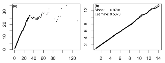
Figure 1. ME plot $\bigl{\{}\bigl{(}X_{(i)},\hat{M}(X_{(i)})\bigr{)},1\leq i\leq 50000\bigr{\}}$ of 50000 random variables from Pareto(2) distribution $(\xi=0.5)$. (a) Entire plot, (b) Order statistics 250-50000.

Figure 1 shows the mean excess plot for this data set. Observe that in Figure 1(a) the first part of the plot is quite linear but it is scattered for very high order statistics. The reason behind this phenomenon is that the empirical mean excess function for high thresholds is the average of the excesses of a small number of upper order statistics. When averaging over few numbers, there is high variability and therefore, this part of the plot appears very non-linear and is uninformative. In Figure 1(b) we zoom into the plot by leaving out the top 250 points. We calculate using all the data but plot only the points $\{(X_{(i)},\hat{M}(X_{(i)})):250\leq i\leq 50000\}$. This restricted plot looks linear. We fit a least squares line to this plot and the estimate of the slope is $0.9701.$ Since the slope is $\xi/(1-\xi)$ we get the estimate of $\xi$ to be $0.5076.$

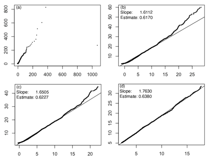
Figure 2. ME plot of 50000 random variables from totally right skewed Stable(1.5) distribution $(\xi=2/3)$. (a) Entire plot, (b) Order statistics 120-30000, (c) 180-20000, (d) 270-10000.

5.1.2. Right-skewed stable distribution

We next simulate 50000 random samples from a totally right skewed stable(1.5) distribution. So $\bar{F}\in RV_{-1.5}$ and then $\xi=2/3$. Figure 2(a) is the ME plot obtained from this data set. This is not a sample from a GPD, but only from a distribution in the maximal domain of attraction of a GPD. The ME function is not exactly linear and for estimating $\xi$ we should concentrate on high thresholds. As we did for the last example we drop points in the plot for very high order statistics since they are the average of a very few values. Figures 2(b), 2(c) and 2(d) confines the plot to the order statistics 120-30000, 180-20000 and 270-10000 respectively, i.e., plots the points $(X_{(i)},\hat{M}(X_{(i)}))$ for $i$ in the specified range. As we restrict the plot more and more, the plot becomes increasingly linear. In Figure 2(d) the least squares estimate of the slope of the line is 1.763 and hence the estimate of $\xi$ is 0.638.

5.1.3. Beta distribution

Figure 3 gives the ME plot for 50000 random variables from the beta(2,2) distribution

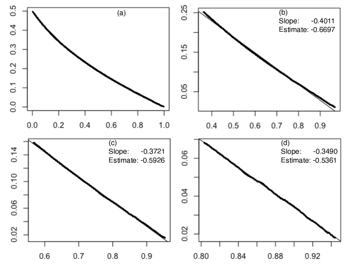
Figure 3. ME Plot of $50000$ random variables from the beta(2,2) distribution $(\xi=-0.5)$. (a) Entire plot, (b) Order statistics: 150-35000, (c) 300-20000, (d) 450-5000.

which is in the maximal domain of the Weibull distribution with the parameter $\xi=-0.5$. Figure 3(a) is the entire ME plot and then Figures 3(b), 3(c) and 3(d) plot the empirical ME function for the order statistics 150-35000, 300-20000 and 450-5000 respectively. The last plot is quite linear and the estimate of $\xi$ is $-0.5361$.

5.2. Difficult Cases

5.2.1. Lognormal distribution

The lognormal(0,1) distribution is in the maximal domain of attraction of the Gumbel and hence $\xi=0$. The ME function of the log normal has the form

$$M(u)=\frac{u}{\ln u}(1+o(1))\ \ \ \ \mbox{ as }u\to\infty;$$

see Table 3.4.7 in (Embrechts et al., 1997, p.161). So $M(u)$ is regularly varying of index $1$ but still $M^{\prime}(u)\to 0$. Figure 4(a) shows the ME plot obtained for a sample of size $10^{5}$ from the lognormal(0,1) distribution.

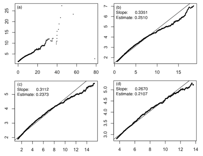
Figure 4. ME plot of $10^{5}$ random variables from the lognormal(0,1) distribution $(\xi=0)$. (a) Entire plot, (b) Order statistics: 150-70000, (c) 300-40000, (d) 450-10000.

Figures 4(b), 4(c) and 4(d) show the empirical ME functions for the order statistics 150-70000, 300-40000 and 450-10000 respectively. The slopes of the least squares lines in Figures 4(b), 4(c) and 4(d) are 0.3351, 0.3112 and 0.267 respectively. The estimate of $\xi$ also decreases steadily as we zoom in towards the higher order statistics from 0.251 in 4(b) to 0.2107 in 4(d). Furthermore, a curve is evident in the plots and the slope of the curve is decreasing, albeit very slowly, as we look at higher and higher thresholds. At a first glance the ME function might seem to resemble that of a distribution in the maximal domain of attraction of the Frechet. The curve becomes evident only after a detailed analysis of the plot. That is possible because the data are simulated but in practice analysis would be difficult. For this example, the ME plot is not a very effective diagnostic for discerning the model.

5.2.2. A non-standard distribution

We also try a non-standard distribution for which $\bar{F}^{-1}(x)=x^{-1/2}(1-10\ln x),0<x\leq 1$. This means that $\bar{F}\in RV_{-2}$ and therefore $\xi=0.5$. The exact form of $\bar{F}$ is given by

(5.1) $$\bar{F}(x)=400W\big{(}xe^{1/20}/20\big{)}^{2}x^{-2}\ \ \ \ \mbox{ for all }x\geq 1,$$

where $W$ is the Lambert W function satisfying $W(x)e^{W(x)}=x$ for all $x>0$. Observe that $W(x)\to\infty$ as $x\to\infty$ and $W(x)\leq\log(x)$ for $x>1$. Furthermore,

$$\frac{\log(x)}{W(x)}=1+\frac{\log W(x)}{W(x)}\to 1\ \ \ \ \mbox{ as }x\to\infty,$$

and hence $W(x)$ is a slowly varying function. This is therefore an example where the slowly varying term contributes significantly to $\bar{F}$. That was not the case in the Pareto or the stable examples.

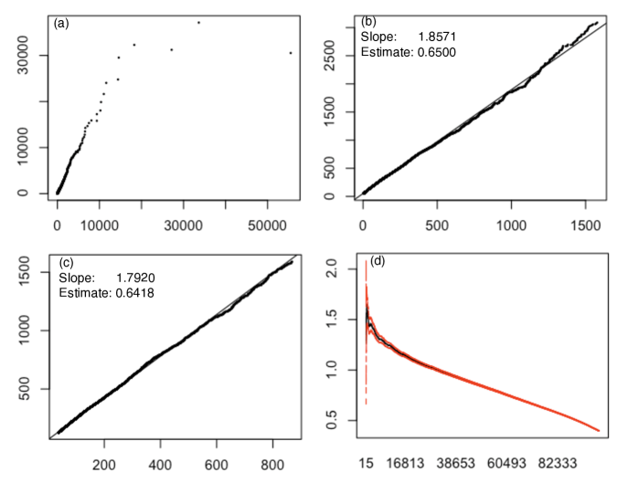
Figure 5. ME Plot of $10^{5}$ random variables from the distribution in (5.1). $(\xi=0.5)$. (a) Entire plot, (b) Order statistics: 150-70000, (c) 400-20000, (d) Hill Plot estimating $\alpha=1/\xi$.

We simulated $10^{5}$ random variables from this distribution. Figure 5(a) gives the entire ME plot from this data set. Figures 5(b) and 5(c) plots the ME function for the order statistics 150-70000 and 400-20000 respectively. In Figure 5(c) the estimate of $\xi$ is 0.6418 which is a somewhat disappointing estimate given that the sample size was $10^{5}$. Figure 5(d) is the Hill Plot from this data set using the QRMlib package in R. It plots the estimate of $\alpha=1/\xi$ obtained by choosing different values of $k$. It is evident from this that the Hill estimator does not perform well here. For none of the values of $k$ is the Hill estimator even close to the true value of $\alpha$ which is 2. We conclude, not surprisingly, that a slowly varying function increasing to infinity can fool both the ME plot and the Hill plot. See Degen et al. (2007) for a discussion on the behavior of the ME plot for a sample simulated from the g-and-h distribution and Resnick (2007) for Hill horror plots.

5.3. Infinite Mean: Pareto with $\xi=2$.

This simulation

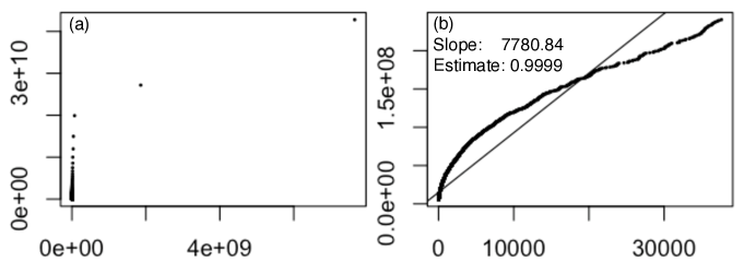
Figure 6. ME plot of 50000 random variables from Pareto(0.5) distribution $(\xi=2)$. (a) Entire plot, (b) Order statistics 250-10000.

sheds light on the behavior of the ME plot when $\xi>1$. In this case the ME function does not exist but the empirical ME plot does. Figure 6 displays the ME plot of for 50000 random variables simulated from Pareto(0.5) distribution. The plot is certainly far from linear even for high order statistics and the least squares line has slope 7780.84 which gives an estimate of $\xi$ to be 0.9999. This certainly gives an indication that the ME plot is not a good diagnostic in this case.

6. ME Plots for Real Data

6.1. Size of Internet Response

This data set consists of Internet response sizes corresponding to user requests. The sizes are thresholded to be at least 100KB. The data set a part of a bigger set collected in April 2000 at the University of North Carolina at Chapel Hill.

Figure 7 contains various plots of the data. Figures 7(b) and Figure 7(e) are the Hill plot (estimating $1/\xi$) and the Pickands plot respectively. It is difficult to infer anything from these plots though superficially they appear stable.

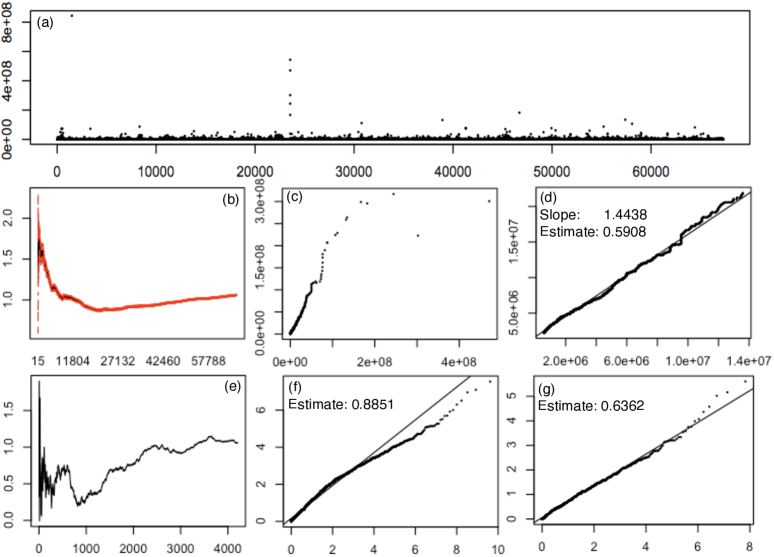
Figure 7. Internet response sizes. (a) Scatter plot, (b) Hill Plot estimating $\alpha=1/\xi$, (c) ME plot, (d) ME plot for order statistics 300-12500, (e) Pickands Plot for $\xi$, (f) QQ plot with $k=15000$, (g) QQ plot with $k=5000$.

Figures 7(c) and 7(d) are the entire ME plot and the ME plot restricted for order statistics 300-12500. The second plot does seem to be very linear and gives an estimate of $\xi$ to be 0.5908. Figures 7(f) and 7(g) are the QQ plots for the data for $k=15000$ and $k=2500$ (as explained in Section 4). The estimate of $\xi$ in these two plots are 0.8851 and 0.6362. The estimates of $\xi$ obtained from the QQ plot 7(d) and the ME plot 7(g) are close and the plots are also linear. So we believe that this is a reasonable estimate of $\xi$.

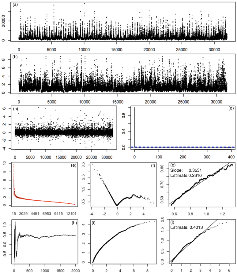
Figure 8. Daily discharge of water in Hudson river. (a) Time series plot, (b) Homoscedasticized plot, (c) Residual plot, (d) ACF of residuals, (e) Hill plot for $\alpha=1/\xi$, (f) ME plot, (g) ME plot for order statistics 300-1300, (h) Pickands plot, (i) QQ plot with $k=8000$, (j) QQ plot with $k=600$.

6.2. Volume of Water in the Hudson River

We now analyze data on the average daily discharge of water (in cubic feet per second) in the Hudson river measured at the U.S. Geological Survey site number 01318500 near Hadley, NY. The range of the data is from July 15, 1921 to December 31, 2008 for a total of 31946 data points.

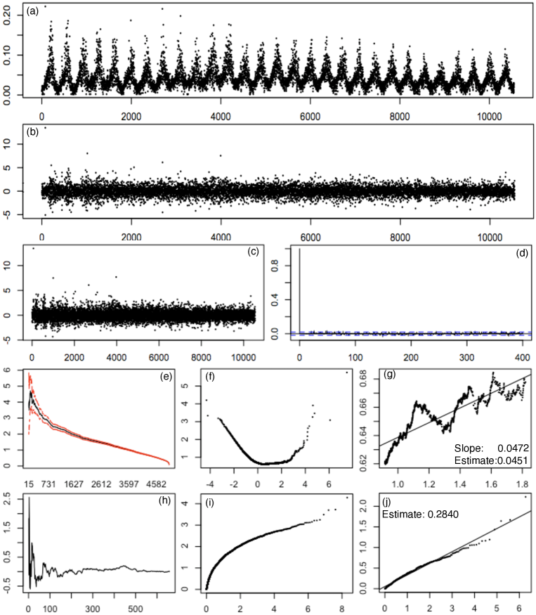
Figure 9. Ozone level in New York City. (a) Time series plot, (b) Homoscedasticized plot, (c) Residual plot, (d) ACF of residuals, (e) Hill plot for $\alpha=1/\xi$, (f) ME plot, (g) ME plot for order statistics 300-1300, (h) Pickands plot, (i) QQ plot with $k=4000$, (j) QQ plot with $k=550$.

Figure 8(a) is the time series plot of the original data and it shows the presence of periodicity in the data. The volume of water is typically much higher in April and May than the rest of the year which possibly is due to snow melt. We ‘homoscedasticize’ the data in the following way. We compute the standard deviation of the average discharge of water for every day of the year and then divide each data point by the standard deviation corresponding to that day. If the original data is say $(X_{7/15/1921},\cdots,X_{12/31/2008})$ then we transform it to $(X_{7/15/1921}/S_{7/15},\cdots,X_{12/31/2008}/S_{12/31})$, where $S_{7/15}$ is the standard deviation of the data points obtained on July 15 in the different years in the range of the data and similarly $S_{12/31}$ is the same for December 31. The plot of the transformed points is given in 8(b). We then fit an AR(33) model to this data using the function ar in the stats package in R. The lag was chosen based on the AIC criterion. Figures 8(c) and (d) show the residuals and their ACF plot respectively. This encourages us to assume that there no linear dependence in the residuals.

We now apply the tools for extreme value analysis on the residuals. Figure 8(e) is the Hill plot and it is difficult to draw any inference from this plot in this case. Figures 8(f) and 8(g) are the entire ME plot and the ME plot restricted to the order statistics 300-1300. From 8(g) we get an estimate of $\xi$ to be 0.261. The Pickands plot in 8(h) and the QQ plots in 8(i) and 8(j) suggest an estimate of $\xi$ around 0.4. A definite curve is visible in the QQ plot even for $k=600$. But the slope of the least squares line fitting the QQ plot supports the estimate suggested by the Pickands plot and the ME plot. We see that it is difficult to reach a conclusion about the range of $\xi$. Still we infer that 0.4 is a reasonable estimate of $\xi$ for this data since that is being suggested by two different methods.

6.3. Ozone level in New York City

We also apply the methods to a data set obtained from http://www.epa.gov/ttn/airs/aqsdatamart. This is the data on daily maxima of level of Ozone (in parts per million) in New York City on measurements closest to the ground level observed between January 1, 1980 and December 31, 2008.

Figure 9(a) is the time series plot of the data. This data set also showed a seasonal component which accounted for high values during the summer months. We transform the data set to a homoscedastic series (Figure 9(b)) using the same technique as explained in Subsection 6.2. Fitting an AR(16) model we get the residuals which are uncorrelated; see Figures 9(c) and 9(d).

The Hill plot in Figure 9(e) again fails to give a reasonable estimate of the tail index. The ME plots in Figures 9(e) and 9(g) are also very rough. Figure 9(g) is the plot of the points $(X_{(i)},\hat{M}(X_{i}))$ for $300\leq i\leq 1300$ and the least squares line fitting these points has slope 0.0472 which gives an estimate of $\xi$ to be 0.0451. This is consistent with the Pickands plot in 9(h). This suggests that the residuals may be in the domain of attraction of the Gumbel distribution.

7. Conclusion.

The ME plot may be used as a diagnostic to aid in tail or quantile estimation for risk management and other extreme value problems. However, some problems associated with its use certainly exist:

• One needs to trim away $\{(X_{(i)},\hat{M}(X_{(i)}))\}$ for small values of $i$ where too few terms are averaged and also trim irrelevent terms for large values of $i$ which are governed by either the center of the distribution or the left tail. So two discretionary cuts to the data need be made whereas for other diagnostics only one threshold needs to be selected.

• The analyst needs to be convinced $\xi<1$ since for $\xi\geq 1$ random sets are the limits for the normalized ME plot. Such random limits could create misleading impressions. The Pickands and moment estimators place no such restriction on the range of $\xi$. The QQ method works most easily when $\xi>0$ but can be extended to all $\xi\in\mathbb{R}$. The Hill method requires $\xi>0$.

• Distributions not particularly close to GPD can fool the ME diagnostic. However, fairness requires pointing out that this is true of all the procedures in the extreme value catalogue. In particular, with heavy tail distributions, if a slowly varying factor is attached to a Pareto tail, diagnostics typically perform poorly.

The standing assumption for the proofs in this paper is that $\{X_{n}\}$ is iid. We believe most of the results on the ME plot hold under the assumption that the underlying sequence $\{X_{n}\}$ is stationary and the tail empirical measure is consistent for the limiting GPD distribution of the marginal distribution of $X_{1}$. We intend to look into this further. Other open issues engaging our attention include converses to the consistency of the ME plot and if the slope of the least squares line through the ME plot is a consistent estimator.

We are thankful to the referees and the editors for their valuable and detailed comments.

References

• Benktander and Segerdahl (1960) Benktander, G., Segerdahl, C., 1960. On the analytical representation of claim distributions with special reference to excess of loss reinsurance. In: XVIth International Congress of Actuaries, Brussels.
• Billingsley (1999) Billingsley, P., 1999. Convergence of Probability Measures, 2nd Edition. John Wiley and Sons, New York.
• Bingham et al. (1989) Bingham, N. H., Goldie, C. M., Teugels, J. L., 1989. Regular Variation. Cambridge University Press.
• Coles (2001) Coles, S., 2001. An Introduction to Statistical Modeling of Extreme Values. Springer-Verlag, London.
• Csorgo and Mason (1986) Csorgo, S., Mason, D., 1986. The asymptotic distribution of sums of extreme values from a regularly varying distribution. The Annals of Probability 14 (3), 974–983.
• Das and Resnick (2008) Das, B., Resnick, S., 2008. Qq plots, random sets and data from a heavy tailed distribution. Stochastic Models 24 (1), 103–132.
• Davison and Smith (1990) Davison, A., Smith, R., 1990. Models for exceedances over high thresholds. Journal of the Royal Statistical Society Series B 52 (3), 393–42.
• de Haan (1976) de Haan, L., 1976. An Abel-Tauber theorem for Laplace transforms. Journal of the London Mathematical Society 13, 537–542.
• de Haan and Ferreira (2006) de Haan, L., Ferreira, A., 2006. Extreme Value Theory: An Introduction. Springer-Verlag, New York.
• de Haan and Peng (1998) de Haan, L., Peng, L., 1998. Comparison of tail index estimators. Statistica Neerlandica 52 (1), 60–70.
• Degen et al. (2007) Degen, M., Embrechts, P., Lambrigger, D. D., 2007. The quantitative modeling of operational risk: between g-and-h and evt. Astin Bulletin 37 (2), 265.
• Dekkers et al. (1989) Dekkers, A., Einmahl, J., de Haan, L., 1989. A moment estimator for the index of an extreme-value distribution. Ann. Statist. 17, 1833–1855.
• Embrechts et al. (1997) Embrechts, P., Klüppelberg, C., Mikosch, T., 1997. Modelling Extremal Events. Vol. 33 of Applications in Mathematics. Springer-Verlag, New York.
• Embrechts et al. (2005) Embrechts, P., McNeil, A. J., Frey, R., 2005. Quantitative Risk Management: Concepts, Techniques, and Tools. Princeton University Press.
• Guess and Proschan (1985) Guess, F., Proschan, F., 1985. Mean Residual Life: Theory and Applications. Defense Technical Information Center.
• Hall and Wellner (1981) Hall, W., Wellner, J., 1981. Mean residual life. Statistics and Related Topics, 169–184.
• Hogg and Klugman (1984) Hogg, R., Klugman, S., 1984. Loss Distributions. Wiley, New York.
• Kratz and Resnick (1996) Kratz, M., Resnick, S., 1996. The qq-estimator and heavy tails. Stochastic Models 12 (4), 699–724.
• Matheron (1975) Matheron, G., 1975. Random Sets and Integral Geometry. Wiley, New York.
• Molchanov (2005) Molchanov, I. S., 2005. Theory of Random Sets. Springer.
• Resnick (2007) Resnick, S., 2007. Heavy-Tail Phenomena: Probabilistic And Statistical Modeling. Springer.
• Resnick and Starica (1998) Resnick, S., Starica, C., 1998. Tail index estimation for dependent data. The Annals of Applied Probability, 1156–1183.
• Resnick (1987) Resnick, S. I., 1987. Extreme Values, Regular Variation and Point Processes. Springer-Verlag, Berlin, New York.
• Smith (1989) Smith, R., 1989. Extreme value analysis of environmental time series: an application to trend detection in ground-level ozone. Statistical Science 4 (4), 367–377.
• Todorovic and Rousselle (1971) Todorovic, P., Rousselle, J., 1971. Some problems of flood analysis. Water Resources Research 7 (5), 1144–1150.
• Todorovic and Zelenhasic (1970) Todorovic, P., Zelenhasic, E., 1970. A stochastic model for flood analysis. Water Resources Research 6 (6), 1641–1648.
• Yang (1978) Yang, G., 1978. Estimation of a biometric function. The Annals of Statistics 6 (1), 112–116.