A possible mechanism of energy dissipation in the front of a shock wave driven ahead of a coronal mass ejection

Abstract

Mark 4 and LASCO C2, C3 coronagraph data analysis shows that, up to the distance $R\sim$ 5 R_⊙ from the center of the Sun, the thickness of a CME-generated shock front may be of order of the proton mean free path. This means that the energy dissipation mechanism in a shock front at these distances is collisional.

Gindraft=false ESELEVICH AND ESELEVICH A POSSIBLE MECHANISM OF ENERGY DISSIPATION M. V. Eselevich, Institute of Solar-Terrestrial physics, Lermontova str. 126a, P.O.Box 291, Irkutsk, 664033, Russia. (mesel@iszf.irk.ru) V. G. Eselevich, Institute of Solar-Terrestrial physics, Lermontova str. 126a, P.O.Box 291, Irkutsk, 664033, Russia. (esel@iszf.irk.ru)

1 Introduction

Eselevich M. and V. (Eselevich and Eselevich, 2008) revealed that there is a disturbed region extended along the direction of coronal mass ejection (CME) propagation in front of the CME, when its velocity $u$ relative to the ambient coronal plasma is below a certain critical velocity $u_{C}$. Given $u>u_{C}$, a discontinuity in the difference brightness distributions is formed in the frontal part of the disturbed region. Since $u_{C}$ is close to the local fast-mode MHD velocity the formation of such a discontinuity may be associated with shock wave formation. If we managed to resolve this discontinuity in space, determining its thickness $\delta_{F}$ (by measuring the shock front profile, in essence), we could be able to clarify the dissipation mechanism in the shock front in the corona.

The purpose of this paper is: 1) to justify the correctness of $\delta_{F}$ measurements in the solar corona using Mark 4 and LASCO C2; 2) to discuss a possible dissipation mechanism in the shock front based on measurements of the shock wave thickness $\delta_{F}$.

2 Method of analysis

This analysis involved coronal images obtained by LASCO C2 and C3 onboard the SOHO spacecraft (Brueckner et al., 1995), presented as difference brightness $\Delta P=P(t)-P(t_{0})$, where $P(t_{0})$ is undisturbed brightness at a moment $t_{0}$, before the event considered; $P(t)$ is disturbed brightness at $t>t_{0}$. We used calibrated LASCO images with the total brightness $P(t)$ expressed in units of the mean solar brightness (P_msb).

The difference brightness images were employed to study the dynamics of the CME and its disturbed region. For this purpose, we used maps of $\Delta P$ isolines as well as sections along the Sun’s radius at fixed position angles $PA$ and non-radial sections at various times. In the images, the position angle $PA$ was counterclockwise from the Sun’s northern pole.

At 1.2 R${}_{\odot}<R<2$ R_⊙, we employed polarization brightness images from the ground-based coronagraph-polarimeter Mark 4 (Mauna Loa Solar Observatory). As was the case with LASCO data, these images were expressed in terms of difference brightness.

3 Identification of the shock front in front of a CME

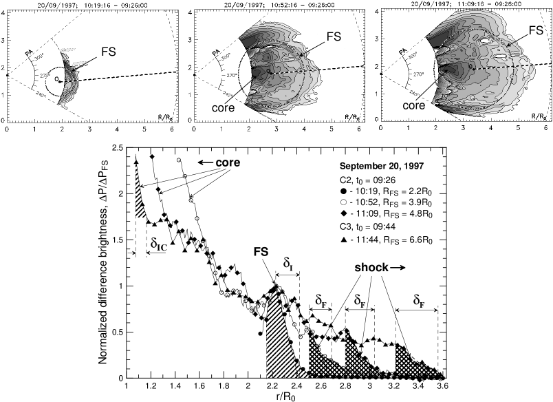
Figure 1: CME 1, 20 September 1997, from LASCO C2 and C3 data. Top panels present difference brightness images for three instants of time. The bottom panel shows difference brightness distributions at successive instants of time starting from the frontal structure center in the directions indicated by the dashed line in the top panels. These distributions are plotted in the coordinate system of the frontal structure and normalized to the frontal structure brightness at the very first instant of time.

To identify a shock front in CME images is best done by tracing the process of its formation. Let us examine such a process on the example of CME 1, which occurred at the W limb on 20 September 1997 at about 10:00 UT. In that event, the coronal ejection had a distinct three-part structure consisting of a frontal structure (FS), cavity, and bright core. Figure 1 (three top panels) presents the difference brightness in the form of isolines for three subsequent instants of time corresponding to the CME motion. The shape of the CME frontal structure is close to a circle (dotted circle in Figure 1).

The process of shock wave formation can be seen in detail on difference brightness distributions $\Delta P(t,R)=P(t,R)-P(t_{0},R)$ plotted along the direction of the CME motion (dashed line in the top panels of Figure 1). Each difference brightness distribution $\Delta P(t,R)$ plotted at a given instant was (see bottom panel in Figure 1):

1. normalized to a corresponding maximum value of difference brightness measured in the vicinity of the frontal structure;

2. displaced along the distance axis $r$ in such a way that the frontal structure position on the axis coincided with its position at the moment of its first registration by LASCO C2. Thus the coordinate system was tied with the frontal structure.

The disturbed region is almost absent at the initial instant (solid circles) in front of the frontal structure (slanting hatching in the figure). At the next moment (empty circles) a compressed plasma region emerges in front of the FS, bounded by the shock in its frontal part (crosshatching). The shock moves faster than the frontal structure and at subsequent moments of time (diamonds and triangles) is seen to be far ahead of the frontal structure. Conversely, the anterior boundary of the core lags behind the frontal structure, because of a lower velocity.

4 Current sheet and how it is different from the shock front

Any density inhomogeneity in the magnetized coronal plasma can only be stationary thanks to magnetic field inhomogeneity, which is equivalent to the presence of current on the same scale. The thickness of quiescent current sheet $\delta_{I}$ expanding due to diffusion can be estimated, via time $t$, from the following relation (Dinklage et al., 2005):

$$\delta_{I}\approx\rho_{e}\sqrt{t/\tau_{ep}}$$

where $\tau_{ep}\approx 10^{-2}T^{3/2}/N$ is the mean time between electron-proton collisions (here $T$ in degrees and $N$ in cm^-3). Let us estimate $\delta_{I}$ for our conditions. Assuming, in accordance with Mann et al. (1999), that, at $R\approx$ 2.1 R_⊙, plasma temperature $T\approx 1.4\times 10^{6}$ K, magnetic field $B\approx$ 0.55 G, and density $N\approx 5\times 10^{6}$ cm^-3 we obtain $\rho_{e}\sim 10^{-9}$ R_⊙ and $\tau_{ep}\approx$ 3 s. Hence during CME propagation in the corona (for several hours), the current sheet thickness does not exceed $\sim 100\rho_{e}$ ($\sim 10^{-7}$ R_⊙) which is much less than the spatial resolution of Mark 4 and C2 ($\sim$ 0.02 R_⊙). This means that the minimal measured current sheet thickness is, at best, close to the spatial resolution of the instruments in use.

However, the motion of the whole current sheet generates in front a disturbed region due to piled-up background plasma particles and to excitation of plasma density and magnetic field variations. In this case, the image brightness jump corresponding to the current sheet will have an enhanced size due to the effect of the disturbed region.

The brightness jump in the shock front is also related to the density inhomogeneity on the scale of the front. Inherently, however, it differs significantly from the current sheet: deceleration and heating of the supersonic plasma stream occur in the shock front. A disturbed region is absent ahead of the shock front as it moves at supersonic speed relative to the environment, and hence the shock front profile does not undergo distortions.

We determined the current sheet thickness at the frontal structure boundary as double the size of the brightness jump at half the jump height ($\delta_{I}$ in the bottom panel in Figure 1). Besides, it is possible to determine the current sheet thickness $\delta_{IC}$ at the core boundary. This value is shown in Figure 1 only schematically, because the maximum core brightness, which, in reality, is much larger, was intentionally limited in the plot. Similarly, Figure 1 illustrates the determination of the thickness of a shock front the brightness jump in which has a typical size $\delta_{F}$.

To understand how we can distinguish the current sheet from a shock wave, let us consider CME 2 that occurred at the W limb on 2 June 1998 at about 08:00 UT. In that event (in contrast to the event of 20 September 1997), the CME velocity was lower than the critical one, and no shock wave formation was observed, at least in the C2 field of view (i.e. up to $\approx$ 6 R_⊙). The top panel in Figure 2 shows the difference brightness at 10:05 UT for the event. A three-part structure (FS, cavity and core) may also be discerned in the event, but there was a rather extended disturbed region in front of the CME in the direction of its motion.

Approximating the shape of the frontal structure as a circle (dots in the top panel of Figure 2) enables us to determine how the current sheet size changes at the front boundary of the frontal structure in various directions. For this purpose, we plotted difference brightness sections from the frontal structure center. These sections were used to estimate the current sheet size $\delta_{I}$. The position of each of these sections was specified by the angle $\alpha$ drawn from the frontal structure center. This angle was measured from the direction of CME propagation. The change in this angle is positive counterclockwise.

In the bottom panel of Figure 2, black circles indicate the dependence of $\delta_{I}$ on angle $\alpha$ for CME 2 at 10:05 UT. There was a developed disturbed region ahead of the frontal structure (the maximum distance of the frontal structure was $\approx$ 3.5 R_⊙). As a result, $\delta_{I}$ was nearly five times as large in the direction of the CME motion than in lateral directions ($\alpha\approx\pm 100^{\circ}$) (Figure 2, solid circles). In CME 1 at 10:19 UT (the maximum distance of the frontal structure from the solar center at this instant was $\approx$ 2.2 R_⊙), the shock front was not observed yet, and $\delta_{I}$ could also be determined at various angles (empty circles in the bottom panel in Figure 2). The $\delta_{I}$ thickness is seen to be approximately constant (0.15 R_⊙), only increasing about twofold in the direction of CME motion ($\alpha\approx 0^{\circ}$).

Hence the development of a disturbed region may result in increased apparent thickness $\delta_{I}$. The disturbed region is only slightly visible and $\delta_{I}$ is the smallest at large angles $\alpha$ (in lateral directions).

A similar angle $\alpha$ dependence can also be plotted for the shock front thickness $\delta_{F}$. In the bottom panel of Figure 2, crosses mark the $\delta_{F}(\alpha)$ plot for CME 1 at 11:09 UT, when the maximum distance of the shock front was $\approx$ 4.8 R_⊙. Obviously, the behavior of $\delta_{F}(\alpha)$ differs from that of $\delta_{I}(\alpha)$. This difference may be due to the lack of a disturbed region ahead of the shock front. In that case, the shock front thickness may depend on local parameters of the ambient plasma as well as on the velocity component along the normal to the shock front (which decreases with increasing angle $\alpha$) – the shock wave type may change in that case.

5 Estimating the resolution

What is the minimum thickness to be recorded by Mark 4 and LASCO C2 for the current sheet in the corona?

Evidently the effect of widening in the optically thin corona will be smallest for the current sheet whose size is smallest along the line of sight. An example is the boundary of the erupting filament in the form of a thin loop, whose size is sufficiently small along the line of sight.

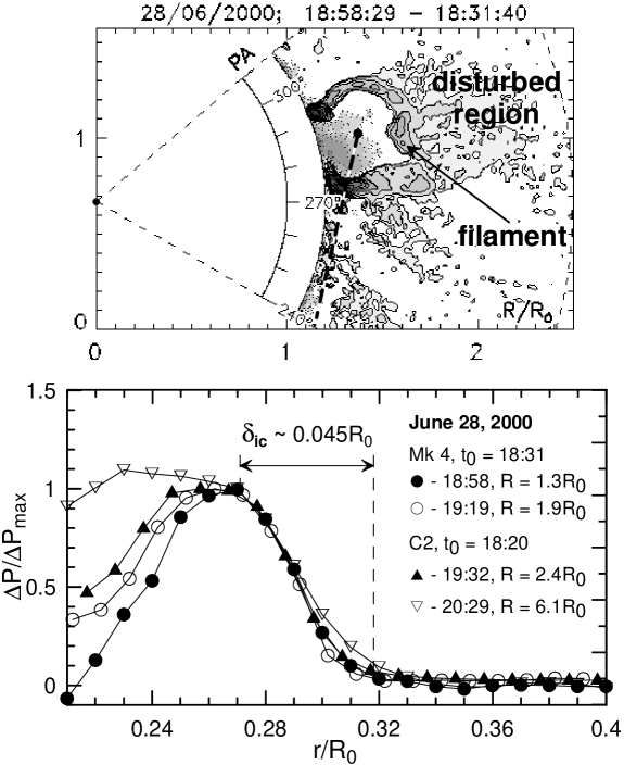
Figure 3: CME with filament eruption on 28 June 2000. Top panel: difference brightness image at 18:59 UT (Mark 4 data). Bottom panel: difference brightness distributions across the filament in the lateral direction at various moments during the eruption (Mark 4 and LASCO C2 data).

The top panel in Figure 3 presents the difference polarization brightness from Mark 4 data for the CME that commenced at the W limb on 28 June 2000 at about 19:00 UT. In that event one could observe a filament eruption easily discernible both in Mark 4 and LASCO C2 images. This event allows us to estimate and compare the Mark 4 and C2 resolutions. For the purpose, we plotted difference brightness profiles across the filament loop along the dashed line passing through the filament center (Figure 3, top panel). Difference brightness profiles normalized to the maximum brightness and shifted in such a manner that their maxima coincided (bottom panel in Figure 3). The plot shows that the spatial size of the brightness jump at the filament boundary remains constant, $\delta_{IC}\approx$ 0.045 R_⊙, over the entire range $R\approx$ 1.3 R_⊙ to $R\approx$ 6.1 R_⊙. This value is close to the spatial resolution of Mark 4 and C2 ($\sim$ 0.02 R_⊙).

The main contribution to the jump widening appears to be by the disturbed region. Thus it is possible to assume that the observable shock wave thickness ($\delta_{F}\sim$ 0.2 R_⊙ in the bottom panel of Figure 2) reflects its real size, as there are no disturbances ahead of the shock front, while the measured shock wave thickness is essentially larger than the spatial resolution of the instrument.

Notably, calculations for a simple geometric model of quasi-spherical shock (Eselevich and Eselevich, 2008) show that the observable brightness profile width $\delta_{F}$ was close to width $\delta_{N}$ for the density jump in the shock wave.

6 Discussion of the energy dissipation mechanism in the shock wave

The measured front size $\delta_{F}$ allows us to answer the question of whether the mechanism of energy dissipation in the shock wave is collisionless (Sagdeev, 1964) or collisional (Zel’dovich and Raizer, 1966).

If it is collisionless, energy dissipation in a shock wave is conditioned by collective processes in plasma due to developing instabilities. In this case, it is quasi-parallel shocks that have maximum front thickness in the magnetized plasma, that does not exceed

$$\delta^{\ast}\approx(10-100)\rho_{p}$$

where $\rho_{p}$ is the proton Larmor radius calculated from undisturbed magnetic field directly ahead of the front (Eselevich, 1983).

To estimate the Larmor radius, we take the coronal magnetic field $B\approx$ 0.5 G and the proton velocity $V=3\times 10^{3}$ km/s for the fastest CME case. We have: $\delta^{\ast}\approx 100\rho_{p}\sim 10^{-4}$ R${}_{\odot}\ll\delta_{F}$. Obviously, the collisionless shock wave front thickness is well below the resolution limit of modern coronagraphs. Measurements show, however, that the front thickness far exceeds this value. This suggests that the dissipation mechanism in the shock wave is collisional in the corona. In this case, the shock wave energy dissipation is on the scale of order of the proton mean free path $\lambda_{p}$ and hence it is also the scale that determines the shock wave thickness (Zel’dovich and Raizer, 1966).

The proton mean free path expressed in solar radii is (Dinklage et al., 2005):

$$\lambda_{p}\approx 10^{-7}T^{2}/N$$ (1)

where $T$ and $N$ are respectively the proton temperature (degrees) and density (cm^-3) in the undisturbed plasma immediately ahead of the shock front.

Compare the observable shock wave front thickness $\delta_{F}$ with $\lambda_{p}$ in the corona. The upper dashed curve in Figure 4 is for $\lambda_{p}$ calculated for the proton temperature and density measured by Strachan et al. (2002). The lower dashed line is for $\lambda_{p}$ calculated for the same density and the temperature half as high as the measurements ($\sim 10^{6}$ K at 2 R_⊙), but suffering the same decay with distance. These two dashed curves define roughly the lower and upper boundaries in estimating the free path depending on the chosen temperature.

The experimental dependence $\delta_{F}(R)$ was plotted from the shock wave front thickness measured at different distances for eight CMEs with velocities $u>u_{C}$ (symbols in Figure 4). The mean curve fitting these data is the thin solid line in Figure 4. The characteristic front size is comparable with the free path ($\delta_{F}\sim\lambda_{p}$), at least up to $\sim$5 R_⊙. This confirms the assumption that the dissipation mechanism in the shock wave may be collisional at these distances. The condition $\delta_{F}\sim\lambda_{p}$ is no valid at greater distances and the shock wave must become collisionless. We did observe a gradual transition to formation of a collisionless shock front with thickness $\delta_{F}^{\ast}\ll\lambda_{p}$ at $R\geq$ 10 R_⊙. This will be dealt with in more detail in a future paper.

Thus, we appear to encounter a rare situation where we can resolve and examine the collisional shock front structure in plasma.

7 Conclusions

The measured thickness of the shock wave, excited ahead of a CME, far exceeds the spatial resolution of Mark 4 and LASCO C2 coronagraphs. Up to the distance $R\sim$ 5 R_⊙ from the center of the Sun the thickness is of order of the proton mean free path. This means that the energy dissipation mechanism in a shock front is collisional.

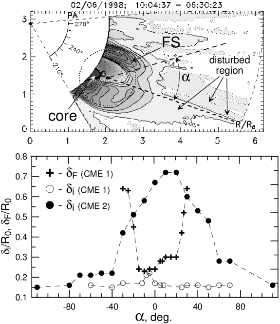
Figure 2: The top panel presents difference brightness images for CME 2 at 10:05 UT on 2 June 1998. The bottom panel: variation in the observable size of the brightness jump depending on the angle $\alpha$ measured from the direction of CME propagation at the CME 1 shock front boundary at 11:44 UT (crosses), CME 1 frontal structure boundary at 10:19 UT (empty circles), CME 2 frontal structure boundary at 10:05 UT (solid circles).

Figure 4: The CME-generated shock wave thickness $\delta_{F}$ variation with distance $R$ from the solar center, in eight CMEs with high velocities: empty squares – 20 September 1997, $PA$ = 20^∘; solid circles – 11 June 1998, $PA$ = 80^∘; crosses – 3 March 2000, PA = 230^∘; solid triangles – 28 June 2000, $PA$ = 270^∘; solid diamonds – 22 November 2001, $PA$ = 247-254^∘; empty triangles – 21 April 2002, $PA$ = 270^∘; empty diamonds – 26 October 2003, $PA$ = 265-290^∘; empty circles – 4 November 2003, $PA$ = 238^∘ (from Mark 4 and LASCO C2, C3 data). The dashed curves are the proton mean free path $\lambda_{p}$ calculated for two proton temperatures.