Bayesian Inference on QGARCH Model Using the Adaptive Construction Scheme

Abstract

We study the performance of the adaptive construction scheme for a Bayesian inference on the Quadratic GARCH model which introduces the asymmetry in time series dynamics. In the adaptive construction scheme a proposal density in the Metropolis-Hastings algorithm is constructed adaptively by changing the parameters of the density to fit the posterior density. Using artificial QGARCH data we infer the QGARCH parameters by applying the adaptive construction scheme to the Bayesian inference of QGARCH model. We find that the adaptive construction scheme samples QGARCH parameters effectively, i.e. correlations between the sampled data are very small. We conclude that the adaptive construction scheme is an efficient method to the Bayesian estimation of the QGARCH model.

1 Introduction

A notable feature of financial time series is that volatility of asset returns varies in time and high (low) volatility persists, which is called volatility clustering. Moreover the return distributions show fat-tailed distributions. These empirical properties are called stylized facts. There also exist further stylized facts seen in financial markets[1].

A primary importance in empirical finance is to make models which mimic the properties of the volatility and then to forecast future volatility. The most successful model is the Generalized Autoregressive Conditional Heteroscedasticity (GARCH) model by Engle[2] and Bollerslev[3], which can capture the property of volatility clustering and show the fat-tailed distribution.

In the original GARCH model, the process generates symmetric time series. For stock markets, however, stock returns may show significant negative skewness in volatility dynamics. In order to incorporate the skewness into the model, some modified models have been proposed[4, 5, 6, 7]. Among them we focus on the Quadratic GARCH (QGARCH) model[6, 7] which includes an additional term that can capture the property of the skewness.

A preferred algorithm to infer GARCH model parameters is the Maximum Likelihood (ML) method which estimates the parameters by maximaizing the corresponding likelihood function of the GARCH model. In this algorithm, however, there is a practical difficulty in the maximization procedure when the output results are sensitive to starting values.

By the recent computer development the Bayesian inference implemeneted by Markov Chain Monte Carlo (MCMC) methods, which is an alternative approach to estimate GARCH parameters, has become popular. There exists a variety of methods proposed to implement the MCMC scheme[8]-[13]. In a recent survey[12] it is shown that Acceptance-Rejection/Metropolis-Hastings (AR/MH) algorithm works better than other algorithms. In the AR/MH algorithm the proposal density is assumed to be a multivariate Student’s t-distribution and the parameters to specify the distribution are estimated by the ML technique. Recently an alternative method to estimate those parameters without relying on the ML technique was proposed [14]. In this method the parameters are determined by using the data generated by an MCMC method and updated adaptively during the MCMC simulation. We call this method ”adaptive construction scheme”.

The adaptive construction scheme was tested for artificial GARCH data and it is shown that the adaptive construction scheme can significantly reduce the correlation between sampled data[14]. In this study we apply the adaptive construction scheme to the QGARCH model. The orignal GARCH model has 3 model parameters. On other hand the QGARCH model has 4 model parameters. We study the efficiency of the adaptive construction scheme applied to the QGARCH model and examine whether the efficiency is still high enough for such a model with many parameters.

2 QGARCH Model

The QGARCH model[6, 7] which we employ here is written as

$$y_{t}=\sigma_{t}\epsilon_{t},$$ (1)

$$\sigma_{t}^{2}=\omega+\gamma y_{t-1}+\alpha y_{t-1}^{2}+\beta\sigma_{t-1}^{2},$$ (2)

where $\epsilon_{t}$ is an independent normal error $\sim N(0,1)$ and $y_{t}$ are observations. Here $\alpha,\beta,\gamma$ and $\omega$ are the parameters to be estimated in the Bayesian inference. The QGARCH process differs from the GARCH one by the term $\gamma y_{t-1}$ which introduces asymmetry.

3 Bayesian inference

From the Bayes’ theorem the posterior density $\pi(\theta|y)$ with $n$ observations $y=(y_{1},y_{2},\dots,y_{n})$ is given by

$$\pi(\theta|y)\propto L(y|\theta)\pi(\theta),$$ (3)

where $L(y|\theta)$ is the likelihood function. $\pi(\theta)$ is the prior density for $\theta$. The functional form of $\pi(\theta)$ is not known a priori. Here we assume that the prior density $\pi(\theta)$ is constant.

For the QGARCH model the likelihood function is given by

$$L(y|\theta)=\Pi_{i=1}^{n}\frac{1}{\sqrt{2\pi\sigma_{t}^{2}}}\exp\left.(-\frac{y_{t}^{2}}{\sigma_{t}^{2}}\right.),$$ (4)

where $\theta=(\omega,\alpha,\beta,\gamma)$ stands for the QGARCH parameters.

Using $\pi(\theta|y)$ the QGARCH parameters are inferred as the expectation values given by

$$\langle{\bf\theta}\rangle=\frac{1}{Z}\int{\bf\theta}\pi(\theta|y)d\theta,$$ (5)

where $Z=\int\pi(\theta|y)d\theta$ is a normalization constant irrelevant to MCMC estimations.

The MCMC technique gives a method to estimate eq.(5) numerically. The basic procedure of the MCMC method is as follows. First we sample $\theta$ drawn from a probability distribution $\pi(\theta|y)$. Sampling is done by a technique which produces a Markov chain. After sampling some data, we evaluate the expectation value as an average value over the sampled data $\theta^{(i)}$,

$$\langle{\bf\theta}\rangle=\lim_{k\rightarrow\infty}\frac{1}{k}\sum_{i=1}^{k}\theta^{(i)},$$ (6)

where $k$ is the number of the sampled data. The statistical error for $k$ independent data is proportional to $\frac{1}{\sqrt{k}}$. In general, however, the data generated by the MCMC method are correlated. As a result the statistical error will be proportional to $\sqrt{\frac{2\tau}{k}}$ where $\tau$ is the autocorrelation time between the sampled data. The autocorrelation time depends on the MCMC method we employ. Thus it is desirable to choose a MCMC method which can generate data with a small $\tau$.

3.1 Metropolis-Hastings algorithm

The MH algorithm[16] is a generalized version of the Metropolis algorithm[15]. Let us consider to generate data $x$ from a probability distribution $P(x)$. The MH algorithm consists of the following steps. First starting from $x$, we propose a candidate $x^{\prime}$ which is drawn from a certain probability distribution $g(x^{\prime}|x)$ which we call proposal density. Then we accept the candidate $x^{\prime}$ with a probability $P_{MH}(x,x^{\prime})$ as the next value of the Markov chain:

$$P_{MH}(x,x^{\prime})=\min\left[1,\frac{P(x^{\prime})}{P(x)}\frac{g(x|x^{\prime})}{g(x^{\prime}|x)}\right].$$ (7)

If $x^{\prime}$ is rejected we keep the previous value $x$. Then we repeat these steps.

4 Adaptive construction scheme

By choosing an adequate proposal density for the MH algorithm one may reduce the correlation between the sampled data. The posterior density of GARCH parameters often resembles to a Gaussian-like shape. Thus one may choose a density similar to a Gaussian distribution as the proposal density. Such attempts have been done by Mitsui, Watanabe[11] and Asai[12]. They used a multivariate Student’s t-distribution in order to cover the tails of the posterior density and determined the parameters to specify the distribution by using the ML technique. Here we also use a multivariate Student’s t-distribution but determine the parameters through MCMC simulations.

The ($p$-dimensional) multivariate Student’s t-distribution is given by

$$g(\theta) = \frac{\Gamma((\nu+p)/2)/\Gamma(\nu/2)}{\det\Sigma^{1/2}(\nu\pi)^{p/2}}$$ (8)

$$\times\left[1+\frac{(\theta-M)^{t}\Sigma^{-1}(\theta-M)}{\nu}\right]^{-(\nu+p)/2},$$

where $\theta$ and $M$ are column vectors,

$$\theta=\left[\begin{array}[]{c}\theta_{1}\\ \theta_{2}\\ \vdots\\ \theta_{p}\end{array}\right],M=\left[\begin{array}[]{c}M_{1}\\ M_{2}\\ \vdots\\ M_{p}\end{array}\right],$$ (9)

and $M_{i}=E(\theta_{i})$. $\displaystyle\Sigma$ is the covariance matrix defined as

$$\frac{\nu\Sigma}{\nu-2}=E[(\theta-M)(\theta-M)^{t}].$$ (10)

$\nu$ is a parameter to tune the shape of Student’s t-distribution. When $\nu\rightarrow\infty$ the Student’s t-distribution goes to a Gaussian distribution. At small $\nu$ Student’s t-distribution has a fat-tail. We also define the matrix $V$ by $\displaystyle V=E[(\theta-M)(\theta-M)^{t}]$ for later use.

There are 4 parameters in the QGARCH model. Thus $p=4$, $\displaystyle\theta=(\theta_{1},\theta_{2},\theta_{3},\theta_{4})=(\alpha,\beta,\omega,\gamma)$ and, $\Sigma$ and $V$ are $4\times 4$ matrices. The unknown parameters in $M$ and $\Sigma$ are determined by using the data obtained from MCMC simulations. First we make a short run by the Metropolis algorithm and accumulate some data. Then we estimate $M$ and $\Sigma$. Note that there is no need to estimate $M$ and $\Sigma$ accurately. Second we perform a MH simulation with the proposal density of eq.(8) with the estimated $M$ and $\Sigma$. After accumulating more data, we recalculate $M$ and $\Sigma$, and update $M$ and $\Sigma$ of eq.(8). By doing this, we adaptively change the shape of eq.(8) to fit the posterior density. We call eq.(8) with the estimated $M$ and $\Sigma$ ”adaptive proposal density”.

5 Numerical results

We examine the adaptive construction scheme by using artificial QGARCH data generated with known parameters. The QGARCH parameters are set to $\alpha=0.07$, $\beta=0.8$, $\gamma=-0.05$ and $\omega=0.1$. We have generated 2000 data by the QGARCH process with these parameters as displayed in Fig.1.

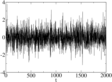
Figure 1: The times series generated by the QGARCH process with $\alpha=0.07$, $\beta=0.8$, $\gamma=-0.05$ and $\omega=0.1$.

The adaptive construction scheme is implemented as follows. First we start a run by the Metropolis algorithm. The first 3000 data are discarded as burn-in process or in other words thermalization. Then we accumulate 1000 data for $M$ and $\Sigma$ estimations. The estimated $M$ and $\Sigma$ are substituted to $g(\theta)$. In this study we take $\nu=10$. We re-start a run by the MH algorithm with $g(\theta)$. Every 1000 updates we re-calculate $M$ and $\Sigma$ and update $g(\theta)$. We accumulate 100000 data for analysis.

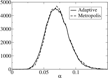
Figure 2: Histograms of $\alpha$ from the adaptive construction scheme and the Metropolis algorithm.

For comparison we also use a standard Metropolis algorithm to infer the GARCH parameters and accumulate 100000 data for analysis.

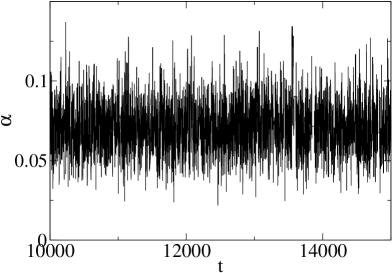
Figure 3: Monte Carlo history of $\alpha$ from the adaptive construction scheme.

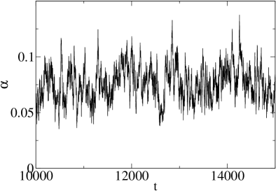
Figure 4: Monte Carlo history of $\alpha$ from the Metropolis algorithm.

TABLE I: Results of QGARCH parameters. SD and SE stand for standard deviation and statistical error respectively.

	$\alpha$	$\beta$	$\omega$	$\gamma$
true	0.07	0.8	0.1	-0.05
Adaptive	0.07143	0.7905	0.1054	-0.04643
SD	0.018	0.056	0.035	0.019
SE	0.00012	0.0005	0.0004	0.00010
$2\tau$	$4.1\pm 1.3$	$10\pm 5.0$	$11\pm 5.1$	$3.0\pm 0.4$
Metropolis	0.0704	0.7943	0.1032	-0.0465
SD	0.018	0.053	0.033	0.019
SE	0.0011	0.0052	0.0032	0.0004
$2\tau$	$340\pm 100$	$840\pm 280$	$820\pm 290$	$54\pm 7$

The results of the parameters inferred by the adaptive construction scheme and Metropolis algorithm are summarized in Table 1.

Fig. 2 compares the histogram of the sampled data $\alpha$ by the adaptive construction scheme with that by the Metropolis algorithm. The histograms from the two MCMC techniques seem to coincide each others. However the property of the sampled data is very different, which will be analyzed in the followings.

Fig. 3-4 show Monte Carlo time histories from the adaptive construction scheme and Metropolis algorithm. It is clearly seen that the data sampled by the Metropolis algorithm are substantially correlated. The similar behavior is also seen for the sampled data for other parameters.

The correlations between the data can be measured by the autocorrelation function (ACF). The ACF of certain successive data $\theta^{(i)}$ is defined by

$$ACF(t)=\frac{\frac{1}{N}\sum_{j=1}^{N}(\theta^{(j)}-\langle\theta\rangle)(\theta^{(j+t)}-\langle\theta\rangle)}{\sigma^{2}_{\theta}},$$ (11)

where $\langle\theta\rangle$ and $\sigma^{2}_{\theta}$ are the average value and the variance of $\theta$ respectively.

Fig. 5-6 show the ACF of $\alpha$ sampled from the adaptive construction scheme and the Metropolis algorithm. The ACF of the adaptive construction scheme decreases quickly as Monte Carlo time $t$ increases. On the other hand the ACF of the Metropolis algorithm decreases very slowly which indicates that the correlation between the sampled data is very large.

The autocorrelation time (ACT) $\tau$ is calculated by

$$\tau=\frac{1}{2}+\sum_{i=1}^{\infty}ACF(i).$$ (12)

Results of $\tau$ are summarized in Table 1. We find that the ACT from the adaptive construction scheme have much smaller $\tau$ than those from the Metropolis simulations. For instance $\tau$ of $\alpha$ parameter from the adaptive construction scheme is decreased by a factor of 90 compared to that from the Metropolis algorithm. These results prove that the adaptive construction scheme is an efficient algorithm for sampling de-correlated data. The differences in $\tau$ also explain that the statistical errors from the adaptive construction scheme are much smaller than those from the Metropolis simulations.

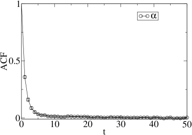
Figure 5: Autocorrelation function of $\alpha$ sampled by the adaptive construction scheme.

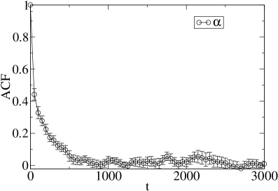
Figure 6: Autocorrelation function of $\alpha$ sampled by the Metropolis algorithm.

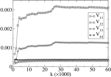
Figure 7: The diagonal elements of $V$ as a function of the data size.

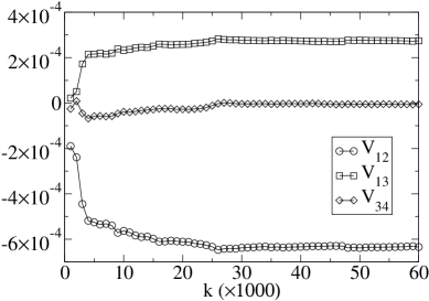
Figure 8: Some off-diagonal elements of $V$ as a function of the data size. Other off-diagonal elements show the similar convergence behavior.

Fig. 7-8 show the convergence property of the covariance matrix $V$. All the elements of $V$ seem to converge to certain values as the simulations are proceeded.

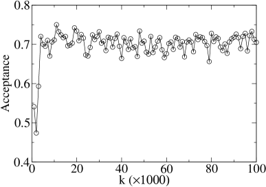
Figure 9: Acceptance at MH step with the adaptive proposal density.

Fig. 9 shows values of the acceptance at the MH algorithm with the adaptive proposal density of eq.(8). Each acceptance is calculated every 1000 updates and the calculation of the acceptance is based on the latest 1000 data. At the first stage of the simulation the acceptance is low. This is because $M$ and $\Sigma$ have not yet been calculated accurately as we see in Fig. 7-8. However the acceptances increase quickly as the simulations are proceeded and reaches plateaus of about $70\%$. This acceptance is reasonably high for the MH algorithm.

6 Conclusions

We have performed the Bayesian inference of the QGARCH model by applying the adaptive construction scheme to the MH algorithm. The adaptive construction scheme, which does not use the ML method, is found to be very efficient in the sense that the autocorrelation times of the sampled data are very small. Thus the adaptive construction scheme serves as an efficient MCMC technique for the Bayesian inference of the QGARCH model. The adaptive construction scheme is not limited to the Bayesian inference of the QGARCH or GARCH models and can be applied for other GARCH-type models.

Although we have updated the parameters of the Student’s t-distribution adaptively using the sampled data during the simlation, we may take a strategy that we stop to update the parameters at some point. As seen in fig. 9, the acceptance quickly reaches a plateau of about $70\%$ and after that the adaptive parameter update does not improve the acceptance. Thus we may stop to update the parameters and use the fixed proposal density for the MH step after the acceptance reaches the plateau.

References

- [1] See e.g., R. Cont Empirical Properties of Asset Returns: Stylized Facts and Statistical Issues. Quantitative Finance 1, 223–236 (2001)
- [2] R.F. Engle, Autoregressive Conditional Heteroskedasticity with Estimates of the Variance. of the United Kingdom inflation. Econometrica 60, 987–1007 (1982)
- [3] T. Bollerslev, Generalized Autoregressive Conditional Heteroskedasticity. Journal of Econometrics 31, 307–327 (1986)
- [4] D.B. Nelson, Conditional Heteroskedasticity in Asset Returns: A New Approach. Econometrica 59, 347–370 (1991)
- [5] L.R. Glston, R. Jaganathan, D.E. Runkle, On the Relation Between the Expected Value and the Volatility of the Nominal Excess on Stocks. Journal of Finance 48, 1779–1801 (1993)
- [6] R.F. Engle, V. Ng, Measuring and testing the impact of news on volatility. Journal of Finance 48, 1749–1778 (1993)
- [7] E. Sentana, Quadratic ARCH models. Review of Economic Studies 62, 639–661 (1995)
- [8] L. Bauwens, M. Lubrano, Bayesian inference on GARCH models using the Gibbs sampler. Econometrics Journal 1, c23-c46 (1998)
- [9] S. Kim, N. Shephard, S. Chib, Stochastic volatility: Likelihood inference and comparison with ARCH models. Review of Economic Studies 65, 361–393 (1998)
- [10] T. Nakatsuma, Bayesian analysis of ARMA-GARCH models: Markov chain sampling approach. Journal of Econometrics 95, 57–69 (2000)
- [11] H. Mitsui, T. Watanabe, Bayesian analysis of GARCH option pricing models. J. Japan Statist. Soc. (Japanese Issue) 33, 307–324 (2003)
- [12] M. Asai, Comparison of MCMC Methods for Estimating GARCH Models. J. Japan Statist. Soc. 36, 199–212 (2006)
-
[13]
T. Takaishi, Bayesian Estimation of GARCH model by Hybrid Monte Carlo.
Proceedings of the 9th Joint Conference on Information Sciences 2006, CIEF-214
doi:10.2991/jcis.2006.159 - [14] T. Takaishi, An Adaptive Markov Chain Monte Carlo Method for GARCH Model. arXiv:0901.0992v1
- [15] N. Metropolis, A.W. Rosenbluth, M.N. Rosenbluth, A.H. Teller, E. Teller, Equations of State Calculations by Fast Computing Machines. J. of Chem. Phys. 21, 1087–1091 (1953)
- [16] W.K. Hastings, Monte Carlo Sampling Methods Using Markov Chains and Their Applications. Biometrika 57, 97–109 (1970)