Radio emission from acceleration sites of solar flares

Abstract

The Letter takes up a question of what radio emission is produced by electrons at the very acceleration site of a solar flare. Specifically, we calculate incoherent radio emission produced within two competing acceleration models—stochastic acceleration by cascading MHD turbulence and regular acceleration in collapsing magnetic traps. Our analysis clearly demonstrates that the radio emission from the acceleration sites: (i) has sufficiently strong intensity to be observed by currently available radio instruments and (ii) has spectra and light curves which are distinctly different in these two competing models, which makes them observationally distinguishable. In particular, we suggest that some of the narrowband microwave and decimeter continuum bursts may be a signature of the stochastic acceleration in solar flares.

1 Introduction

Acceleration of charged particles is an internal property of energy release in solar flares, which has not yet been fully understood in spite of a significant progress achieved recently (e.g., Aschwanden, 2002; Vilmer & MacKinnon, 2003). A traditional way of getting information on the accelerated electrons in flares is the analysis of the hard X-ray (HXR) emission produced by nonthermal bremsstrahlung. However, because the bremsstrahlung intensity increases with the density of the ambient plasma, it is likely that in most cases the acceleration site and HXR emission site are spatially separated; therefore, the HXR emission does not carry direct information on the acceleration site. This concept of distinct acceleration, propagation, and emission regions was then inherited by solar radio astronomy (e.g., Fig. 9 in Bastian et al., 1998), which looks relevant to relatively weak events of electron acceleration visualized by coherent emission of type III groups and of accompanying metric spikes (e.g., Fig. 10 in Bastian et al., 1998).

However, it is well known that a charged particle produces electromagnetic emission as it moves with acceleration. Stated another way, fast electrons must produce radiation immediately at the acceleration region with intensity and other characteristics defined by type of the acceleration, or more precisely, by the type of fast electron trajectories in the acceleration region. We show in this Letter that typically this emission has a spectral peak at the microwave range, which makes the radio observation the most suitable to study the acceleration region in flares.

By now, a huge variety of acceleration mechanisms and models has been proposed and developed for the solar flares. Acceleration by DC electric fields, both sub-Dreicer and super-Dreicer, (Holman, 1985; Tsuneta, 1985; Holman & Benka, 1992; Litvinenko, 1996, 2000, 2003); stochastic acceleration by turbulent waves (Hamilton & Petrosian, 1992; Petrosian et al., 1994; Miller et al., 1996; Miller, 1997; Park et al., 1997; Pryadko & Petrosian, 1998; Bykov & Fleishman, 2009), the classical diffusive shock acceleration (Aschwanden, 2002); the regular (betatron plus Fermi) acceleration in collapsing magnetic traps (Somov & Kosugi, 1997; Somov & Bogachev, 2003; Karlický & Kosugi, 2004; Bogachev & Somov, 2005, 2007, 2009); all are currently considered in the context of solar flares.

To illustrate potential ability of radio observations to detect the radiation from the flare acceleration site and to distinguish then between competing acceleration mechanisms, we calculate here radio emission generated within two distinct acceleration models—stochastic acceleration by a turbulence spectrum and regular acceleration in collapsing traps. Radio emission of flares is known to be produced by a variety of emission mechanisms including gyrosynchrotron (GS) emission, bremsstrahlung, transition radiation, and a number of coherent radiative processes (Bastian et al., 1998; Nindos et al., 2008). Some of the observed emission types can in fact originate from acceleration sites, while others—from electrons trapped in closed magnetic loops or from electrons propagating along open field lines. Based on our analysis, we suggest that some of the narrowband microwave and decimeter continuum bursts may be a signature of the stochastic acceleration in solar flares, while the collapsing trap acceleration must reveal itself in drifting to higher frequencies microwave GS bursts.

2 Radio Emission from a Region of Stochastic Acceleration

Basically, various models of stochastic acceleration differ from each other by the accelerating agent (the plasma or MHD eigen-mode responsible for the wave-particle energy exchange) and presence or absence of some pre-acceleration (injection) process. To be specific, we assume a ’pure’ stochastic acceleration process when the electrons are accelerated directly from the thermal pool (Hamilton & Petrosian, 1992; Miller et al., 1996), perhaps as a result of MHD turbulence cascading towards the smallest scales involved into resonant interaction of the waves with thermal or weakly superthermal electrons.

Within this model the MHD turbulence is created at some large scale and then a broad spectrum of the turbulence develops due to the turbulence cascading. As soon as small-scale waves capable of resonant interaction with electrons from Maxwellian tail are produced they start to accelerate those electrons. This process can be modeled by growing a power-law tail (sf., e.g. spectra of accelerated electrons presented by Hamilton & Petrosian, 1992; Miller et al., 1996; Bykov & Fleishman, 2009)

$$N(E)=(\delta(t)-1)\frac{n(>E_{0})\cdot E_{0}^{\delta(t)-1}}{E^{\delta(t)}}\exp\left(-\frac{E}{E_{br}(t)}\right),$$ (1)

where the time-dependent acceleration is modeled by increasing the break energy $E_{br}(t)$ and hardening the energy spectrum (decreasing spectral index $\delta(t)$). This nonthermal distribution of accelerated electrons is assumed to match the original Maxwellian distribution at a certain energy $E_{0}$; $n(>E_{0})$ is evidently defined by the matching condition:

$$n(>E_{0})=\frac{2n_{e}}{\delta(t)-1}\sqrt{\frac{E_{0}^{3}}{\pi(kT_{e})^{3}}}\cdot\exp\left(\frac{-E_{0}}{kT_{e}}\right)\exp\left(\frac{E_{0}}{E_{br}(t)}\right),$$ (2)

where $n_{e}$ and $T_{e}$ are the number density and temperature of the thermal electrons, $k$ is the Boltzman constant. Figure 1 shows a sequence of the electron spectra as the electron acceleration progresses.

Figure 1: Distribution function of electrons for different $\delta$ and the following parameters: the thermal electron number density $n_{e}=10^{10}$ cm^-3; the electron temperature $T_{e}=10^{6}$ K; the matching energy is $E_{0}=6kT_{e}$. The solid curve denotes the original Maxwellian distribution.

Let us consider the radio emission produced by accelerated electrons with the spectrum (1) at the acceleration region. We note that gyrosynchrotron (GS) emission by nonrelativistic and weakly relativistic electrons available during an initial phase of the acceleration modeled by Eq. (1) is inefficient; the flux of the GS emission remains typically very small until sufficient number of electrons is accelerated up to a few hundred keV (Bastian et al., 1998). However, along with the regular magnetic field, there is a spectrum of turbulent waves (those accelerating the electrons) at the acceleration site. The nonthermal electrons, interacting with those random waves, experience spatial diffusion and so produce so called Diffusive Synchrotron Radiation (DSR, Fleishman, 2006), which we calculate here.

Neglecting for simplicity the plasma gyrotropy we can take the refractive index of the radio waves in the form

$$n_{\sigma}=\sqrt{\varepsilon},\qquad\varepsilon = 1-\frac{\omega_{pe}^{2}}{\omega^{2}},\qquad\omega_{pe}=\sqrt{\frac{4\pi e^{2}n_{e}}{m}}.$$ (3)

Then, spectral and angular distribution of the energy radiated by a relativistic charged particle with a given Fourier transformed acceleration $\mathbf{w}_{\omega^{\prime}}$ during time $T$ of the particle motion in an external field is given by (Landau & Lifshitz, 1971)

$${\cal E}_{{\bf n},\omega}=\sqrt{\varepsilon}\frac{Q^{2}}{c^{3}}\left(\frac{\omega}{\omega^{\prime}}\right)^{4}\left|\left[{\bf n}\left[\left({\bf n}-\frac{\bf v}{c}\right){\bf w}_{\omega^{\prime}}\right]\right]\right|^{2},$$ (4)

where

$$\omega^{\prime}=\omega\left(1-\frac{{\bf nv}}{c}\sqrt{\varepsilon(\omega)}\right).$$ (5)

In the nonrelativistic case $v/c\ll 1$ ($\gamma\equiv\sqrt{1-v^{2}/c^{2}}\approx 1$) and $\omega^{\prime}\approx\omega$, Eq. (4) reduces to

$${\cal E}_{{\bf n},\omega}=\sqrt{\varepsilon}\frac{Q^{2}}{c^{3}}\left|\left[{\bf n}\times{\bf w}_{\omega}\right]\right|^{2},$$ (6)

where $Q$ is the particle charge and ${\bf n}$ is the unit wave vector of the radiation. Eq. (6) shows that the radiation in a given direction ${\bf n}$ is defined by the acceleration component $\left|{\bf w}_{\omega\bot}\right|^{2}=\left|\left[{\bf n}\times{\bf w}_{\omega}\right]\right|^{2}$ transverse to ${\bf n}$. Similarly to the derivation in ultrarelativistic case (Fleishman, 2006), the transverse component of the acceleration can be expressed via temporal and spatial Fourier transform of the external Lorentz force, $F^{\alpha}_{q_{0},{\bf q}}$

$$\mid{\bf w}_{\omega\bot}\mid^{2}=\frac{(2\pi)^{3}}{M^{2}V}\int dq_{0}d{\bf q}\delta(\omega-q_{0}+{\bf qv})(\delta_{\alpha\beta}-n_{\alpha}n_{\beta})F^{\alpha}_{q_{0},{\bf q}}F^{\beta*}_{q_{0},{\bf q}},$$ (7)

where $M$ is the mass of emitting particle and $V$ is the source volume.

For electric component of the Lorenz force $\mathbf{F}=Q\mathbf{E}$ we have

$$(\delta_{\alpha\beta}-n_{\alpha}n_{\beta})F^{\alpha}_{q_{0},{\bf q}}F^{\beta*}_{q_{0},{\bf q}}=Q^{2}(\delta_{\alpha\beta}-n_{\alpha}n_{\beta})E^{\alpha}_{q_{0},{\bf q}}E^{\beta*}_{q_{0},{\bf q}},$$ (8)

where

$$E^{\alpha}_{q_{0},{\bf q}}E^{\beta*}_{q_{0},{\bf q}}=\frac{TV}{(2\pi)^{4}}K_{\alpha\beta}(q_{0},{\bf q}),$$ (9)

$K_{\alpha\beta}(q_{0},{\bf q})$ is the correlation tensor of the random electric field, such as $\int dq_{0}d{\bf q}K_{\alpha\alpha}(q_{0},{\bf q})=\left<E_{st}^{2}\right>$ (Toptygin, 1985).

For magnetic component of the Lorenz force the corresponding expression is different

$$\begin{array}[]{l}(\delta_{\alpha\beta}-n_{\alpha}n_{\beta})F^{\alpha}_{q_{0},{\bf q}}F^{\beta*}_{q_{0},{\bf q}}=\frac{Q^{2}}{c^{2}}\left(v^{2}\delta_{\alpha\beta}-v_{\alpha}v_{\beta}-[\mathbf{n}\times\mathbf{v}]_{\alpha}[\mathbf{n}\times\mathbf{v}]_{\beta}\right)B^{\alpha}_{q_{0},{\bf q}}B^{\beta*}_{q_{0},{\bf q}}=\\ \\ Q^{2}\frac{v^{2}}{c^{2}}\left(n_{\alpha}n_{\beta}+\frac{({\bf nv})^{2}}{v^{2}}\delta_{\alpha\beta}-({\bf nv})\frac{v_{\alpha}n_{\beta}+n_{\alpha}v_{\beta}}{v^{2}}\right)B^{\alpha}_{q_{0},{\bf q}}B^{\beta*}_{q_{0},{\bf q}}.\end{array}$$ (10)

Similarly to Eq. (9) we have

$$B^{\alpha}_{q_{0},{\bf q}}B^{\beta*}_{q_{0},{\bf q}}=\frac{TV}{(2\pi)^{4}}K_{\alpha\beta}(q_{0},{\bf q}),$$ (11)

where $K_{\alpha\beta}(q_{0},{\bf q})$ is the correlation tensor of the random magnetic field, such as $\int dq_{0}d{\bf q}K_{\alpha\alpha}(q_{0},{\bf q})=\left<B_{st}^{2}\right>$. Thus, the DSR intensity, $I_{\textbf{n},\omega}={\cal E}_{{\bf n},\omega}/T$, of a nonrelativistic particle in the presence of random magnetic field is

$$I_{\textbf{n},\omega}=\sqrt{\varepsilon}\frac{Q^{4}v^{2}}{2\pi M^{2}c^{5}}\int dq_{0}d{\bf q}\delta(\omega-q_{0}+\textbf{qv})\left(n_{\alpha}n_{\beta}+\frac{({\bf nv})^{2}}{v^{2}}\delta_{\alpha\beta}-({\bf nv})\frac{v_{\alpha}n_{\beta}+n_{\alpha}v_{\beta}}{v^{2}}\right)K_{\alpha\beta}(q_{0},{\bf q}).$$ (12)

This expression is valid for arbitrary spectrum of magnetic turbulence including anisotropic distributions.

We consider here the DSR produced by accelerated nonrelativistic electrons interacting with the MHD turbulence. In MHD waves $E\sim(v_{a}/c)B$, where $v_{a}$ is the Alfvén speed, therefore the magnetic part of the Lorenz force is larger than the electric part for all electrons with $v>v_{a}$. Assuming this condition to be fulfilled, we calculate only the DSR related to the magnetic field of the MHD turbulence; inclusion of electric field effect will further increase the DSR intensity.

Since we are interested in overall spectral shapes and flux level of the DSR, rather than model-dependent details of the emission, we consider here the simplest case of the isotropic MHD turbulence:

$$K_{\alpha\beta}=\frac{1}{2}\left({\delta}_{\alpha\beta}-\frac{q_{\alpha}q_{\beta}}{q^{2}}\right)K(\textbf{q})\delta(q_{0}-q_{0}(\textbf{q})).$$ (13)

As we assumed $v>v_{a}$, i.e., the electrons move faster than the waves, we can adopt the MHD turbulence to be quasi static, $q_{0}(\textbf{q})=0$. When the MHD turbulence is isotropic, the accelerated electrons are isotropic as well, and so the radiation produced is also isotropic. Thus, we consider further the radiation produced into the full solid angle

$$I_{\omega}=\int I_{\textbf{n},\omega}d\Omega=\sqrt{\varepsilon}\frac{8Q^{2}}{3\pi c}\cdot q(\omega),$$ (14)

where, like in the ultrarelativistic case (Fleishman, 2006), we introduce the scattering rate of the nonrelativistic particle by MHD turbulence $q(\omega)$:

$$q(\omega)=\frac{\pi}{4}\left(\frac{Q}{Mc}\right)^{2}\frac{v^{2}}{c^{2}}\int K(\textbf{q})\delta(\omega+\textbf{qv})\,{d\textbf{q}}.$$ (15)

To proceed further we have to specify the shape of the turbulence spectrum $K(\textbf{q})$; we adopt a single power-law down to the smallest (resonant to thermal electrons) scales:

$$K(\textbf{q})=\frac{A_{\nu}}{q^{\nu+2}}\qquad A_{\nu}=\frac{\nu-1}{4\pi}k_{0}^{\nu-1}\langle B_{st}^{2}\rangle,$$ (16)

where $k_{0}=2\pi/L_{0}$ with $L_{0}$ the largest turbulence scale, $\langle B_{st}^{2}\rangle$ is the mean square of the turbulent magnetic field, and $\nu$ is the turbulence spectral index.

Then, substituting (16) into (15), integrating over $d\textbf{q}$,

$$\begin{array}[]{l}\int\,{d\textbf{q}}K(\textbf{q})\delta(\omega+\textbf{qv})=2\pi\int\,{d}\cos\theta\cdot\,{d}q\frac{A_{\nu}}{q^{\nu}}\delta(\omega+qv\cos\theta)=\frac{2\pi A_{\nu}}{v}\int\limits_{\frac{\omega}{v}}^{\frac{\omega_{pe}}{v_{pe}}}\frac{\,dq}{q^{\nu+1}}=\\ \frac{2\pi}{\nu}\frac{A_{\nu}}{v}\left(\frac{v}{\omega}\right)^{\nu}\left(1-\left(\frac{\omega v_{pe}}{\omega_{pe}v}\right)^{\nu}\right)\Theta\left(\frac{\omega_{pe}}{v_{pe}}-\frac{\omega}{v}\right)\end{array}$$ (17)

where

$$v_{pe} = 6.74\times 10^{5}\sqrt{T_{e}}$$ (18)

is the thermal velocity of the plasma electrons, $\Theta(x)$ is the step function, and using the electron charge $e$ and mass $m$ for $Q$ and $M$, we find

$$q(\omega)=\frac{\pi^{2}A_{\nu}}{2\nu}\frac{e^{2}v}{m^{2}c^{4}}\left(\frac{v}{\omega}\right)^{\nu}\left(1-\left(\frac{\omega v_{pe}}{\omega_{pe}v}\right)^{\nu}\right)\Theta\left(\frac{\omega_{pe}}{v_{pe}}-\frac{\omega}{v}\right),$$ (19)

so the DSR spectrum produced by accelerated electrons reads

$$I_{\omega} = \frac{8e^{2}}{3\pi c}\sqrt{\varepsilon}\cdot q(\omega).$$ (20)

Now we calculate the DSR power from $N$ electrons with the spectrum described by Eq. (1)

$$P_{\omega}=\int\limits_{E_{0}}^{\infty}I_{\omega}N(E)\,dE.$$ (21)

In fact, we are interested in the radio flux observed at the Earth. To transform this radiation power into the flux observed at the Earth, we change the variable $\omega=2\pi f$, so that $I_{f}=2\pi I_{\omega}$. Then, the flux is

$$F_{f}=\frac{2\pi P_{\omega}V}{4\pi R_{au}^{2}}=\frac{P_{\omega}L^{3}}{2R_{au}^{2}}\cdot 10^{19}\quad{\rm sfu},$$ (22)

where $R_{au}=1$ au$=1.49\times 10^{13}$ cm is the distance from the Earth to the Sun.

To evaluate the DSR from the acceleration region of a solar flare, we adopt some typically assumed parameters of the acceleration site as follows: (a) the size of the site $L\sim 10^{8}$ cm; (b) the thermal electron number density $n_{e}\sim 10^{10}$ cm^-3; (c) the electron temperature $T_{e}\sim 10^{6}$ K; (d) the energy density of the magnetic turbulence $W_{st}=\frac{\langle B_{st}^{2}\rangle}{8\pi}\sim 10^{3}$ erg/cm³. Accordingly, the total energy, $W_{tot}\sim W_{st}L^{3}\sim 10^{27}$ ergs, corresponds to a very modest solar flare. We assume that the power-law tail of the accelerated electrons grows from $E_{0}=(4-6)kT_{e}$ with $n(>E_{0})$ specified by matching condition (2) and as the acceleration has started, the power law index $\delta$ changes from $8\sim 3$ while the break energy $E_{br}$ increases from $50\sim 500$ keV.

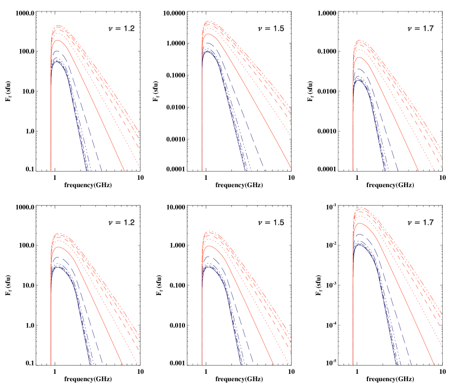
Figure 2: The DSR total flux density spectra calculated for the observations from the Earth surface for $E_{0}=4kT$ (upper panel) and $E_{0}=6kT$ (lower panel) for 11 different $\delta$ from $7\sim 3$ and three different $\nu$, indicated in the panels. The blue curves indicate larger $\delta$, while the red ones show smaller $\delta$.

Figure 2 presents the sequence of calculated DSR spectra for 11 different $\delta$ values from $7\sim 3$; the spectra are calculated for three different $\nu$ values and for two different $E_{0}$ values. The blue curves indicate larger $\delta$, while the red ones show smaller $\delta$. Then, Figure 3(a) presents the DSR spectra for three different temperature values, $T=(1,3,10)\cdot 10^{6}K$. In addition to spectrum shapes, light curves of the radiation at different frequencies can be informative. To estimate the light curve behavior we adopt a soft-hard-soft spectrum evolution as follows from theory of spectrum evolution for the stochastic acceleration (Bykov & Fleishman, 2009), and which is typical for impulsive flares, with the electron energy spectral index $\delta(t)$ changing from 8 to 3 and then back to 8, while the break energy $E_{br}$ increasing all the way from 50 keV to $\sim 1$ MeV. Figure 3(b) shows the corresponding model light curves at a few frequencies around the spectrum peak. One can note from the figure that higher frequency light curves have a somewhat shorter duration, although peaking at the same time; so no appreciable time delay between the light curves is expected.

Figure 3: (a) DSR spectra for three sources with $\delta=7$, $E_{0}=4kT_{e}$, and different electron temperatures, $T_{e}=(1,~{}3,~{}10)\cdot 10^{6}$ K; (b) DSR light curves for the case $E_{0}=4kT_{e}$, $\nu=1.2$, $E_{br}=\left(E_{br}(t=0)+\frac{dE_{br}}{dt}\cdot t\right)$ keV, where $E_{br}(t=0)=50$ keV, $\frac{dE_{br}}{dt}=45$ keV/s, and soft-hard-soft evolution of the accelerated electron spectrum, $\delta=\delta_{\max}+a\cdot(t-t_{0})^{2}$, where $\delta_{\max}=3$, $t_{0}=5$ s, and $a=0.2$ s^-2. The apparent symmetry of the model light curves is provided by assumed symmetry of the spectral index variation and adopted no variation of MHD spectrum; relaxing any of these assumption will result in asymmetric light curves. All the light curves peak almost simultaneously, so no ”cross-correlation” delay is expected, although onset of higher frequency light curves is delayed, thus, the total duration of higher frequency emission is shorter.

We note that the DSR spectra are very narrowband, much narrower that typical gyrosynchrotron spectra. The high frequency slope of the DSR spectrum can easily be evaluated from Eqns. (22), (21), (19), and (20), $F_{f}\propto f^{3-2\delta}$. Thus, the DSR high frequency spectral index varies from 11 to 3 as the spectral index of accelerated electrons changes from 7 to 3, while the GS spectral index would vary from 5 to 1 for the same range of $\delta$ variation. The peak flux of the DSR is highly sensitive to the turbulence spectral index (specified eventually by the MHD cascading law), while less sensitive to the plasma temperature and electron spectral index. The peak flux can be very large (up to a few hundred sfu), which makes it easily observable even by full sun radio instruments. If so, the corresponding radio emission must have been widely observed by available radio spectrometers working in the decimetric and/or microwave range. Indeed, there is a class of radio bursts with the properties resembling the DSR properties described here—it is the class of narrowband decimetric and microwave continuum bursts (including type IVdm), which, we suggest, may contain burst-candidates to the radio emission from the regions of stochastic acceleration in solar flares. Although this interpretation is tempting, spatially resolved radio observations of the DSR will be needed to confirm it, to locate the region of stochastic acceleration, and study it in detail. Another plausible candidate for radio emission from stochastic acceleration episodes is so-called transient brightenings, whose radio spectra are often narrowband (Gary et al., 1997).

3 Gyrosynchrotron Radio Emission from a Collapsing Trap

Let us consider another model, a collapsing magnetic trap, which can efficiently accelerate charged particles. Unlike the stochastic acceleration models, no turbulence spectrum is essential to accelerate particles in the collapsing trap model; however, some spectrum of ’pre-accelerated’ particles is needed, otherwise, the collapse of the trap will only give rise to plasma heating without nonthermal particle generation.

Therefore, we assume that just before collapsing the trap contained both thermal plasma and nonthermal electron population with a power-law spectrum. To be specific, we adopt the initial conditions as follows: (a) the magnetic field strength $B_{0}=30$ G; (b) the minimum and the maximum energy of the power-law spectrum $E_{\rm min}=0.01$ MeV, $E_{\rm max}=1$ MeV; (c) the thermal electron density $n_{th}=10^{9}$ cm^-3 and the non-thermal electron density $n_{rl}=10^{7}$ cm^-3; (d) the source size $L_{0}=10"$.

During the trap contraction, the number of accelerated electrons evolves. For our modeling we adopt a solution obtained by Bogachev & Somov (2005), see Figure 4, which takes into account the betatron and Fermi acceleration and the particle escape from the trap via the loss cone:

$$N=N_{0}\frac{l\sqrt{b_{m}-b}}{\sqrt{1+(b_{m}-1)l^{2}}}$$ (23)

where

$$b=b(t) = B(t)/B_{0}$$ (24)

$$l=l(t) = L(t)/L_{0}$$ (25)

so $b(t)$ changes from $b(0)=1$ to $b_{m}=B_{m}/B_{0}$, $B_{m}$ is the largest magnetic field value at the end of the trap collapse, and $l(t)$ deceases from $l(0)=1$ to a very low value, say, $l(t_{\rm max})=0.1$. For the sake of simplicity we assume a self-similar contraction of the collapsing magnetic trap. In this case, evolution of all parameters of the trap is uniquely defined by their initial values and the dimensionless source scale $l(t)$. Thus, for any given contraction law, $l(t)$, we can easily calculate the corresponding time history of all other relevant source parameters, as the magnetic field, the thermal electron number density, the source volume and the projected area, and the evolution of the nonthermal electron spectrum (Bogachev & Somov, 2005, 2007). For our modeling we adopt that the trap volume $V$ linearly decreases with time during the trap contraction from $10"^{3}$ to $1"^{3}$; we adopt 10 s for the trap collapse time, which is a few Alfven times ($\tau_{a}\sim L/v_{a}$) for the trap parameters used.

Figure 4: Left: The number of electrons in the trap according to the Bogachev & Somov (2005) model. Right: GS spectra in frequency range $0.1\sim 10^{4}$ GHz; the solid spectra are plotted for $t=$ 0, 1, …, 9 s; the dashed-doted lines correspond to the end of collapse at $t=$ 9.75, 9.975, 9.9975 s. In fact, we take into account both GS and free-free contributions to the radiation intensity, however, the free-free component is inessential during the loop collapse: it is only noticeable at high frequency flat regions of the early spectra.

Thus, we can straightforwardly calculate the GS spectra at different time frames and the radio light curves at different frequencies within the adopted collapsing trap model. Figure 4 displays the GS spectra at different moments of the trap contraction. In agreement with a statement made in the previous section, at initial phase of acceleration the GS flux is small (less than 1 sfu), which can only be recorded by high sensitivity spatially resolved observations. However, during the trap contraction the magnetic field increases and the fast electrons are accelerated, which all together lead to a significant increase of the peak flux and the peak frequency of the radio emission produced at the acceleration site; thus the radio emission becomes easily detectable by available radio instrument soon after the trap starts to contract.

Figure 5: The light curves (a) and the normalized light curves (b) of the GS emission from a collapsing trap at a number of fixed frequencies 5, 10, 17, 34 GHz. The initial trap parameters and the contraction law are described in the text. A significant time delay between the light curves, comparable to duration of the light curves, is evident from the Figure.

Figure 5 presents the light curves of the emission at a number of fixed frequencies, 5, 10, 17, 34 GHz. Within the adopted model the peak flux increases with frequency, see Figures 4, 5; in fact, this increase may become less pronounced if the coulomb losses in the collapsing trap are taken into account (Bogachev & Somov, 2009). A distinctive feature of the light curves, contrasting to that of DSR produced from the stochastic acceleration sites, is a noticeable time delay: the higher frequency light curves are delayed relative to lower frequency light curves; this time delay will be present even when the coulomb losses (Bogachev & Somov, 2009) are included. A time delay in the sense predicted by our modeling is frequently observed in solar flares, in particular, in those with quasiperiodic pulsations (Fleishman et al., 2008). Observationally, however, the GS emission from a collapsing trap can be contaminated by GS emission from trapped electrons produced by previous acceleration episodes, so unambiguous detection of the GS emission from a collapsing trap itself requires additional accurate analysis to separate the contributions, which as yet has not been performed.

4 Discussion

There are many models in which electrons can be accelerated to nonthermal energies. Some mechanisms accelerate a tiny fraction of the electrons, which can only be observed via coherent radio emissions (e.g., type III bursts produced by electron beams, or accompanying metric spikes), others produce more powerful acceleration, sufficient to generate observable incoherent radio emission from either the acceleration site itself of from a remote ’radiation site’.

The idea of using radio observations to probe energy release/acceleration regions in flares has been around for awhile (e.g., Bastian et al., 1998), however, the studies focused mainly on coherent decimeter radio bursts. For example, Benz (1986) argued that decimeter narrowband millisecond radio spike clusters can be a signature of electron acceleration in flares, and, if so, the flare energy release must have been highly fragmented with each spike indicating a single energy release/acceleration episode. However, it has been found (Aschwanden & Güdel, 1992) that the radio spikes are frequently delayed compared with associated hard X-ray emission, implying the spikes are a secondary phenomenon associated with flares. Moreover, spatially resolved observations (Benz et al., 2002; Battaglia & Benz, 2009) show that the spike sources are typically far away from main flare locations. Even though higher frequency microwave radio spikes (Fleishman et al., 2003; Rozhansky et al., 2008) can be produced at or around the main flare location (Gary & Naqvi, 2009), it seems doubtful that the coherent radio burst originate from elementary acceleration episodes (Fleishman & Melnikov, 1998; Fleishman et al., 2003; Rozhansky et al., 2008; Battaglia & Benz, 2009).

In contrast, in this Letter we have calculated incoherent radio emission from the acceleration region of a solar flare within two distinct acceleration models—stochastic acceleration by cascading MHD turbulence and regular (betatron and Fermi) acceleration in a collapsing trap. We have demonstrated that the radio emissions produced within these two competing acceleration models are distinctly different, which potentially allows distinguishing between them by the radio observations. In particular, we have found that the stochastic acceleration process is accompanied by a very narrowband DSR continuum radio emission, whose predicted properties are generally consistent with observed properties of narrowband microwave or decimetric (type IVdm) continuum bursts, thus, we suggest that some of those bursts can be produced from the sites of stochastic acceleration.

References

- Asai et al. (2006) Asai, A., Nakajima, H., Shimojo, M., White, S. M., Hudson, H. S., & Lin, R. P. 2006, PASJ, 58, L1
- Aschwanden (2002) Aschwanden, M. J. 2002, Particle Acceleration and Kinematics in Solar Flares (Particle Acceleration and Kinematics in Solar Flares, A Synthesis of Recent Observations and Theoretical Concepts, by Markus J. Aschwanden, Lockheed Martin, Advanced technology Center, palo Alto, California, U.S.A. Reprinted from SPACE SCIENCE REVIEWS, Volume 101, Nos. 1-2 Kluwer Academic Publishers, Dordrecht)
- Aschwanden & Güdel (1992) Aschwanden, M. J. & Güdel, M. 1992, ApJ, 401, 736
- Bastian et al. (1998) Bastian, T. S., Benz, A. O., & Gary, D. E. 1998, ARA&A, 36, 131
- Battaglia & Benz (2009) Battaglia, M. & Benz, A. O. 2009, A&A, 499, L33
- Battaglia et al. (2009) Battaglia, M., Fletcher, L., & Benz, A. O. 2009, A&A, 498, 891
- Benz (1986) Benz, A. O. 1986, Sol. Phys., 104, 99
- Benz et al. (2002) Benz, A. O., Saint-Hilaire, P., & Vilmer, N. 2002, A&A, 383, 678
- Bogachev & Somov (2005) Bogachev, S. A. & Somov, B. V. 2005, Astronomy Letters, 31, 537
- Bogachev & Somov (2007) —. 2007, Astronomy Letters, 33, 54
- Bogachev & Somov (2009) —. 2009, Astronomy Letters, 35, 57
- Bykov & Fleishman (2009) Bykov, A. M. & Fleishman, G. D. 2009, ApJ, 692, L45
- Fleishman (2006) Fleishman, G. D. 2006, ApJ, 638, 348
- Fleishman et al. (2008) Fleishman, G. D., Bastian, T. S., & Gary, D. E. 2008, ApJ, 684, 1433
- Fleishman et al. (2003) Fleishman, G. D., Gary, D. E., & Nita, G. M. 2003, ApJ, 593, 571
- Fleishman & Melnikov (1998) Fleishman, G. D. & Melnikov, V. F. 1998, Uspekhi Fizicheskikh Nauk, 41, 1157
- Gary & Naqvi (2009) Gary, D. E. & Naqvi, M. 2009, AAS Bull., 41, 851
- Gary et al. (1997) Gary, D. E., Hartl, M. D., & Shimizu, T. 1997, ApJ, 477, 958
- Hamilton & Petrosian (1992) Hamilton, R. J. & Petrosian, V. 1992, ApJ, 398, 350
- Holman (1985) Holman, G. D. 1985, ApJ, 293, 584
- Holman & Benka (1992) Holman, G. D. & Benka, S. G. 1992, ApJ, 400, L79
- Karlický & Kosugi (2004) Karlický, M. & Kosugi, T. 2004, A&A, 419, 1159
- Landau & Lifshitz (1971) Landau, L. D. & Lifshitz, E. M. 1971, The classical theory of fields, ed. L. D. Landau & E. M. Lifshitz
- Litvinenko (1996) Litvinenko, Y. E. 1996, ApJ, 462, 997
- Litvinenko (2000) —. 2000, Sol. Phys., 194, 327
- Litvinenko (2003) Litvinenko, Y. E. 2003, in Lecture Notes in Physics, Berlin Springer Verlag, Vol. 612, Energy Conversion and Particle Acceleration in the Solar Corona, ed. L. Klein, 213–229
- Miller (1997) Miller, J. A. 1997, ApJ, 491, 939
- Miller et al. (1996) Miller, J. A., Larosa, T. N., & Moore, R. L. 1996, ApJ, 461, 445
- Nindos et al. (2008) Nindos, A., Aurass, H., Klein, K.-L., & Trottet, G. 2008, Sol. Phys., 253, 3
- Park et al. (1997) Park, B. T., Petrosian, V., & Schwartz, R. A. 1997, ApJ, 489, 358
- Petrosian et al. (1994) Petrosian, V., McTiernan, J. M., & Marschhauser, H. 1994, ApJ, 434, 747
- Pryadko & Petrosian (1998) Pryadko, J. M. & Petrosian, V. 1998, ApJ, 495, 377
- Rozhansky et al. (2008) Rozhansky, I. V., Fleishman, G. D., & Huang, G.-L. 2008, ApJ, 681, 1688
- Somov & Bogachev (2003) Somov, B. V. & Bogachev, S. A. 2003, Astronomy Letters, 29, 621
- Somov & Kosugi (1997) Somov, B. V. & Kosugi, T. 1997, ApJ, 485, 859
- Toptygin (1985) Toptygin, I. N. 1985, Cosmic rays in interplanetary magnetic fields, ed. I. N. Toptygin
- Tsuneta (1985) Tsuneta, S. 1985, ApJ, 290, 353
- Vilmer & MacKinnon (2003) Vilmer, N. & MacKinnon, A. L. 2003, in Lecture Notes in Physics, Berlin Springer Verlag, Vol. 612, Energy Conversion and Particle Acceleration in the Solar Corona, ed. L. Klein, 127–160