Pricing Bermudan options using nonparametric regression: optimal rates of convergence for lower estimates

Abstract

The problem of pricing Bermudan options using Monte Carlo and a nonparametric regression is considered. We derive optimal non-asymptotic bounds for a lower biased estimate based on the suboptimal stopping rule constructed using some estimates of continuation values. These estimates may be of different nature, they may be local or global, with the only requirement being that the deviations of these estimates from the true continuation values can be uniformly bounded in probability. As an illustration, we discuss a class of local polynomial estimates which, under some regularity conditions, yield continuation values estimates possessing this property.

Keywords: Bermudan options, Nonparametric regression, Boundary condition, Suboptimal stopping rule

1 Introduction

An American option grants the holder the right to select the time at which to exercise the option, and in this differs from a European option which may be exercised only at a fixed date. A general class of American option pricing problems can be formulated through an $\mathbb{R}^{d}$ Markov process $\{X(t),\,0\leq t\leq T\}$ defined on a filtered probability space $(\Omega,\mathcal{F},(\mathcal{F}_{t})_{0\leq t\leq T},\operatorname{P})$. It is assumed that $X(t)$ is adapted to $(\mathcal{F}_{t})_{0\leq t\leq T}$ in the sense that each $X_{t}$ is $\mathcal{F}_{t}$ measurable. Recall that each $\mathcal{F}_{t}$ is a $\sigma$-algebra of subsets of $\Omega$ such that $\mathcal{F}_{s}\subseteq\mathcal{F}_{t}\subseteq\mathcal{F}$ for $s\leq t$. We interpret $\mathcal{F}_{t}$ as all relevant financial information available up to time $t$. We restrict attention to options admitting a finite set of exercise opportunities $0=t_{0}<t_{1}<t_{2}<\ldots<t_{L}=T$, sometimes called Bermudan options. If exercised at time $t_{l},\,l=1,\ldots,L$, the option pays $f_{l}(X(t_{l}))$, for some known functions $f_{0},f_{1},\ldots,f_{L}$ mapping $\mathbb{R}^{d}$ into $[0,\infty)$. Let $\mathcal{T}_{n}$ denote the set of stopping times taking values in $\{n,n+1,\ldots,L\}$. A standard result in the theory of contingent claims states that the equilibrium price $V_{n}(x)$ of the American option at time $t_{n}$ in state $x$ given that the option was not exercised prior to $t_{n}$ is its value under an optimal exercise policy:

$$V_{n}(x)=\sup_{\tau\in\mathcal{T}_{n}}\operatorname{E}[f_{\tau}(X(t_{\tau}))|X(t_{n})=x],\quad x\in\mathbb{R}^{d}.$$

Pricing an American option thus reduces to solving an optimal stopping problem. Solving this optimal stopping problem and pricing an American option are straightforward in low dimensions. However, many problems arising in practice (see e.g. Glasserman (2004)) have high dimensions, and these applications have motivated the development of Monte Carlo methods for pricing American option. Pricing American style derivatives with Monte Carlo is a challenging task because the determination of optimal exercise strategies requires a backwards dynamic programming algorithm that appears to be incompatible with the forward nature of Monte Carlo simulation. Much research was focused on the development of fast methods to compute approximations to the optimal exercise policy. Notable examples include the functional optimization approach in Andersen (2000), mesh method of Broadie and Glasserman (1997), the regression-based approaches of Carriere (1996), Longstaff and Schwartz (2001), Tsitsiklis and Van Roy (1999) and Egloff (2005). A common feature of all above mentioned algorithms is that they deliver estimates $\widehat{C}_{0}(x),\ldots,\widehat{C}_{L-1}(x)$ for the so called continuation values:

(1.1) $$C_{k}(x):=\operatorname{E}[V_{k+1}(X(t_{k+1}))|X(t_{k})=x],\quad k=0,\ldots,L-1.$$

An estimate for $V_{0}$, the price of the option at time $t_{0}$ can then be defined as

$$\widetilde{V}_{0}(x):=\max\{f_{0}(x),\widehat{C}_{0}(x)\},\quad x\in\mathbb{R}^{d}.$$

This estimate basically inherits all properties of $\widehat{C}_{0}(x)$. In particular, it is usually impossible to determine the sign of the bias of $\widetilde{V}_{0}$ since the bias of $\widehat{C}_{0}$ may change its sign. One way to get a lower bound (low biased estimate) for $V_{0}$ is to construct a (generally suboptimal) stopping rule

$$\widehat{\tau}=\min\{0\leq k\leq L:\widehat{C}_{k}(X(t_{k}))\leq f_{k}(X(t_{k}))\}$$

with $\widehat{C}_{L}\equiv 0$ by definition. Simulating a new independent set of trajectories and averaging the pay-offs stopped according to $\widehat{\tau}$ on these trajectories gives us a lower bound $\widehat{V}_{0}$ for $V_{0}$. As was observed by practitioners, the so constructed estimate $\widehat{V}_{0}$ has rather stable behavior with respect to the estimates of continuation values $\widehat{C}_{0}(x),\ldots,\widehat{C}_{L-1}(x)$, that is even rather poor estimates of continuation values may lead to a good estimate $\widehat{V}_{0}.$ The aim of this paper is to find a theoretical explanation of this observation and to investigate the properties of $\widehat{V}_{0}$. In particular, we derive optimal non-asymptotic bounds for the bias $V_{0}-\operatorname{E}\widehat{V}_{0}$ assuming some uniform probabilistic bounds for $C_{r}-\widehat{C}_{r}$. It is shown that the bounds for $V_{0}-\operatorname{E}\widehat{V}_{0}$ are usually much tighter than ones for $V_{0}-\operatorname{E}\widetilde{V}_{0}$ implying a better quality of $\widehat{V}_{0}$ as compared to the quality of $\widetilde{V}_{0}$ constructed using one and the same set of estimates for continuation values. As an example, we consider the class of local polynomial estimators for continuation values and derive explicit convergence rates for $\widehat{V}_{0}$ in this case.

The issues of convergence for regression algorithms have been already studied in several papers. Clément, Lamberton and Protter (2002) were first who proved the convergence of the Longstaff-Schwartz algorithm. Glasserman and Yu (2005) have shown that the number of Monte Carlo paths has to be in general exponential in the number of basis functions used for regression in order to ensure convergence. Recently, Egloff, Kohler and Todorovic (2007) have derived the rates of convergence for continuation values estimates obtained by the so called dynamic look-ahead algorithm (see Egloff (2004)) that “interpolates” between Longstaff-Schwartz and Tsitsiklis-Roy algorithms. As was shown in these papers the convergence rates for $\widetilde{V}_{0}$ coincide with the rates of $\widehat{C}_{0}$ and are determined by the smoothness properties of the true continuation values $C_{0},\ldots,C_{L-1}$. It turns out that the convergence rates for $\widehat{V}_{0}$ depend not only on the smoothness of continuation values (as opposite to $\widetilde{V}_{0}$), but also on the behavior of the underlying process near the exercise boundary. Interestingly enough, there are some cases where these rates become almost independent either of the smoothness properties of $\{C_{k}\}$ or of the dimension of $X$ and the bias of $\widehat{V}_{0}$ decreases exponentially in the number of Monte Carlo paths used to construct $\{\widehat{C}_{k}\}$.

The paper is organized as follows. In Section 2.1 we introduce and discuss the so called boundary assumption which describes the behavior of the underlying process $X$ near the exercise boundary and heavily influences the properties of $\widehat{V}_{0}$. In Section 2.2 we derive non-asymptotic bounds for the bias $V_{0}-\operatorname{E}\widehat{V}_{0}$ and prove that these bounds are optimal in the minimax sense. In Section 2.3 we consider the class of local polynomial estimates and propose a sequential algorithm based on the dynamic programming principle to estimate all continuation values. Finally, under some regularity assumptions, we derive exponential bounds for the corresponding continuation values estimates and consequently the bounds for the bias $V_{0}-\operatorname{E}\widehat{V}_{0}$.

2 Main results

2.1 Boundary assumption

For the considered Bermudan option let us introduce a continuation region $\mathcal{C}$ and an exercise (stopping) region $\mathcal{E}$ :

(2.2) $$\mathcal{C} := \left\{(i,x):f_{i}(x)<C_{i}(x)\right\},$$

$$\mathcal{E} := \left\{(i,x):f_{i}(x)\geq C_{i}(x)\right\}.$$

Furthermore, let us assume that there exist constants $B_{0,k}>0$, $k=0,\ldots,L-1$ and $\alpha>0$ such that the inequality

(2.3) $$\operatorname{P}_{t_{k}|t_{0}}(0<|C_{k}(X(t_{k}))-f_{k}(X(t_{k}))|\leq\delta)\leq B_{0,k}\delta^{\alpha},\quad\delta>0,$$

holds for all $k=0,\ldots,L-1$, where $\operatorname{P}_{t_{k}|t_{0}}$ is the conditional distribution of $X(t_{k})$ given $X(t_{0})$. Assumption (2.3) provides a useful characterization of the behavior of the continuation values $\{C_{k}\}$ and payoffs $\{f_{k}\}$ near the exercise boundary $\partial\mathcal{E}$. Although this assumption seems quite natural to look at, we make in this paper, to the best of our knowledge, a first attempt to investigate its influence on the convergence rates of lower bounds based on suboptimal stopping rules. We note that a similar condition, although much simpler, appears in the context of statistical classification problem (see, e.g. Mammen and Tsybakov (1999) and Audibert and Tsybakov (2007)).

In the situation when all functions $C_{k}-f_{k},\,k=0,\ldots,L-1$ are smooth and have non-vanishing derivatives in the vicinity of the exercise boundary, we have $\alpha=1$. Other values of $\alpha$ are possible as well. We illustrate this by two simple examples.

Example 1

Fix some $\alpha>0$ and consider a two period ($L=1$) Bermudan power put option with the payoffs

(2.4) $$f_{0}(x)=f_{1}(x)=(K^{1/\alpha}-x^{1/\alpha})^{+},\quad x\in\mathbb{R}_{+},\quad K>0.$$

Denote by $\Delta$ the length of the exercise period, i.e. $\Delta=t_{1}-t_{0}.$ If the process $X$ follows the Black-Scholes model with volatility $\sigma$ and zero interest rate, then one can show that

$$C_{0}(x):=\operatorname{E}[f_{1}(X(t_{1}))|X(t_{0})=x]=K^{1/\alpha}\Phi(-d_{2})\\ -x^{1/\alpha}e^{\Delta(\alpha^{-1}-1)(\sigma^{2}/2\alpha)}\Phi(-d_{1})$$

with $\Phi$ being the cumulative distribution function of the standard normal distribution,

$$d_{1}=\frac{\log(x/K)+\left(\frac{1}{\alpha}-\frac{1}{2}\right)\sigma^{2}\Delta}{\sigma\sqrt{\Delta}}$$

and $d_{2}=d_{1}-\sigma\sqrt{\Delta}/\alpha.$ As can be easily seen, the function $C_{0}(x)-f_{0}(x)$ satisfies $|C_{0}(x)-f_{0}(x)|\asymp x^{1/\alpha}$ for $x\to+0$ and $C_{0}(x)>f_{0}(x)$ for all $x>0$ if $\alpha\geq 1$. Hence

$$\operatorname{P}(0<|C_{0}(X(t_{0}))-f_{0}(X(t_{0}))|\leq\delta)\lesssim\delta^{\alpha},\quad\delta\to 0,\quad\alpha\geq 1.$$

Taking different $\alpha$ in the definition of the payoffs (2.4), we get (2.3) satisfied for $\alpha$ ranging from $1$ to $\infty$.

Figure 1: Illustration to Example 2.

In fact, even the extreme case “$\alpha=\infty$” may take place as shown in the next example.

Example 2

Let us consider again a two period Bermudan option such that the corresponding continuation value $C_{0}(x)=\operatorname{E}[f_{1}(X(t_{1}))|X(t_{0})=x]$ is positive and monotone increasing function of $x$ on any compact set in $\mathbb{R}$. Fix some $x_{0}\in\mathbb{R}$ and choose $\delta_{0}$ satisfying $\delta_{0}<C_{0}(x_{0})$. Define the payoff function $f_{0}(x)$ in the following way

$$f_{0}(x)=\begin{cases}C_{0}(x_{0})+\delta_{0},&\,x<x_{0},\\ C_{0}(x_{0})-\delta_{0},&\,x\geq x_{0}.\end{cases}$$

So, $f_{0}(x)$ has a “digital” structure. Figure 1 shows the plots of $C_{0}$ and $f_{0}$ in the case where $X$ follows the Black-Scholes model and $f_{1}(x)=(x-K)^{+}$. It is easy to see that

$$\operatorname{P}_{t_{0}}(0<|C_{0}(X(t_{0}))-f_{0}(X(t_{0}))|\leq\delta_{0})=0.$$

On the other hand

$$\mathcal{C} = \{x\in\mathbb{R}:C_{0}(x)\geq f_{0}(x)\}=\{x\in\mathbb{R}:x\geq x_{0}\},$$

$$\mathcal{E} = \{x\in\mathbb{R}:C_{0}(x)<f_{0}(x)\}=\{x\in\mathbb{R}:x<x_{0}\}.$$

So, both continuation and exercise regions are not trivial in this case.

The last example is of particular interest because as will be shown in the next sections the bias of $\widehat{V}_{0}$ decreases in this case exponentially in the number of Monte Carlo paths used to estimate the continuation values, the lower bound $\widehat{V}_{0}$ was constructed from.

2.2 Non-asymptotic bounds for $V_{0}-\operatorname{E}\widehat{V}_{0}$

Let $\widehat{C}_{k,M},\,k=1,\ldots,L-1,$ be some estimates of continuation values obtained using $M$ paths of the underlying process $X$ starting from $x_{0}$ at time $t_{0}$. We may think of $(X^{(1)}(t),\ldots,X^{(M)}(t))$ as being a vector process on the product probability space with $\sigma$-algebra $\mathcal{F}^{\otimes M}$ and the product measure $\operatorname{P}_{x_{0}}^{\otimes M}$ defined on $\mathcal{F}^{\otimes M}$ via

$$\operatorname{P}_{x_{0}}^{\otimes M}(A_{1}\times\ldots\times A_{M})=\operatorname{P}_{x_{0}}(A_{1})\cdot\ldots\cdot\operatorname{P}_{x_{0}}(A_{M}),$$

with $A_{m}\in\mathcal{F},\,m=1,\ldots,M$. Thus, each $\widehat{C}_{k,M},\,k=0,\ldots,L-1,$ is measurable with respect to $\mathcal{F}^{\otimes M}$. The following proposition provides non-asymptotic bounds for the bias $V_{0}-\operatorname{E}_{\operatorname{P}_{x_{0}}^{\otimes M}}[V_{0,M}]$ given uniform probabilistic bounds for $\{\widehat{C}_{k,M}\}$.

Proposition 2.1.

Suppose that there exist constants $B_{1},\,B_{2}$ and a positive sequence $\gamma_{M}$ such that for any $\delta>\delta_{0}>0$ it holds

(2.5) $$\operatorname{P}_{x_{0}}^{\otimes M}\left(|\widehat{C}_{k,M}(x)-C_{k}(x)|\geq\delta\gamma^{-1/2}_{M}\right)\leq B_{1}\exp(-B_{2}\delta)$$

for almost all $x$ with respect to $\operatorname{P}_{t_{k}|t_{0}}$, the conditional distribution of $X(t_{k})$ given $X(t_{0})$, $k=0,\ldots,L-1$. Define

(2.6) $$V_{0,M}:=\operatorname{E}\left[f_{\widehat{\tau}_{M}}(X(t_{\widehat{\tau}_{M}}))|X(t_{0})=x_{0}\right]$$

with

(2.7) $$\widehat{\tau}_{M}:=\min\left\{0\leq k\leq L:\widehat{C}_{k,M}(X(t_{k}))\leq f_{k}(X(t_{k}))\right\}.$$

If the boundary condition (2.3) is fulfilled, then

$$0\leq V_{0}-\operatorname{E}_{\operatorname{P}_{x_{0}}^{\otimes M}}[V_{0,M}]\leq B\left[\sum_{l=0}^{L-1}B_{0,l}\right]\gamma^{-(1+\alpha)/2}_{M}$$

with some constant $B$ depending only on $\alpha$, $B_{1}$ and $B_{2}$.

The above convergence rates can not be in general improved as shown in the next theorem.

Proposition 2.2.

Let $L=2$. Fix a pair of non-zero payoff functions $f_{1},f_{2}$ such that $f_{2}:\mathbb{R}^{d}\to\{0,1\}$ and $0<f_{1}(x)<1$ on $[0,1]^{d}.$ Let $\mathcal{P}_{\alpha}$ be a class of pricing measures such that the boundary condition (2.3) is fulfilled with some $\alpha>0$. For any positive sequence $\gamma_{M}$ satisfying

$$\gamma^{-1}_{M}=o(1),\quad\gamma_{M}=O(M),\quad M\to\infty,$$

there exist a subset $\mathcal{P}_{\alpha,\gamma}$ of $\mathcal{P}_{\alpha}$ and a constant $B>0$ such that for any $M\geq 1$, any stopping rule $\widehat{\tau}_{M}$ and any set of estimates $\{\widehat{C}_{k,M}\}$ measurable w.r.t. $\mathcal{F}^{\otimes M}$, we have for some $\delta>0$ and $k=1,2,$

$$\sup_{\operatorname{P}\in\mathcal{P}_{\alpha,\gamma}}\operatorname{P}^{\otimes M}\left(|\widehat{C}_{k,M}(x)-C_{k}(x)|\geq\delta\gamma^{-1/2}_{M}\right)>0$$

for almost all $x$ w.r.t. any $\operatorname{P}\in\mathcal{P}_{\alpha,\gamma}$ and

$$\sup_{\operatorname{P}\in\mathcal{P}_{\alpha,\gamma}}\left\{\sup_{\tau\in\mathcal{T}_{0}}\operatorname{E}^{\mathcal{F}_{t_{0}}}_{\operatorname{P}}[f_{\tau}(X(t_{\tau}))]-\operatorname{E}_{\operatorname{P}^{\otimes M}}[\operatorname{E}^{\mathcal{F}_{t_{0}}}_{\operatorname{P}}f_{\widehat{\tau}_{M}}(X(t_{\widehat{\tau}_{M}}))]\right\}\geq B\gamma^{-(1+\alpha)/2}_{M}.$$

Finally, we discuss the case when “$\alpha=\infty$”, meaning that there exists $\delta_{0}>0$ such that

(2.8) $$\operatorname{P}_{t_{k}|t_{0}}(0<|C_{k}(X(t_{k}))-f_{k}(X(t_{k}))|\leq\delta_{0})=0$$

for $k=0,\ldots,L-1.$ This is very favorable situation for the pricing of the corresponding Bermudan option. It turns out that if the continuation values estimates $\{\widehat{C}_{k,M}\}$ satisfy a kind of exponential inequality and (2.8) holds, then the bias of $V_{0,M}$ converges to zero exponentially fast in $\gamma_{M}$.

Proposition 2.3.

Suppose that for any $\delta>0$ there exist constants $B_{1},\,B_{2}$ possibly depending on $\delta$ and a sequence of positive numbers $\gamma_{M}$ not depending on $\delta$ such that

(2.9) $$\operatorname{P}_{x_{0}}^{\otimes M}\left(|\widehat{C}_{k,M}(x)-C_{k}(x)|\geq\delta\right)\leq B_{1}\exp(-B_{2}\gamma_{M})$$

for almost all $x$ with respect to $\operatorname{P}_{t_{k}|t_{0}}$, $k=0,\ldots,L-1$. Assume also that there exists a constant $B_{f}>0$ such that

(2.10) $$\operatorname{E}\left[\max_{k=0,\ldots,L}f^{2}_{k}(X(t_{k}))\right]\leq B_{f}.$$

If the condition (2.8) is fulfilled with some $\delta_{0}>0$, then

$$0\leq V_{0}-\operatorname{E}_{\operatorname{P}_{x_{0}}^{\otimes M}}[V_{0,M}]\leq B_{3}L\exp(-B_{4}\gamma_{M})$$

with some constant $B_{3}$ and $B_{4}$ depending only on $B_{1}$, $B_{2}$ and $B_{f}$.

Discussion

Let us make a few remarks on the results of this section. First, Proposition 2.1 implies that the convergence rates of $\widehat{V}_{0,M}$, a Monte Carlo estimate for $V_{0,M}$, are always faster than the convergence rates of $\{\widehat{C}_{k,M}\}$ provided that $\alpha>0$. Indeed, while the convergence rates of $\{\widehat{C}_{k,M}\}$ are of order $\gamma_{M}^{-1/2}$, the bias of $\widehat{V}_{0,M}$ converges to zero as fast as $\gamma_{M}^{-(1+\alpha)/2}.$ As to the variance of $\widehat{V}_{0,M}$, it can be made arbitrary small by averaging $\widehat{V}_{0,M}$ over a large number of sets, each consisting of $M$ trajectories, and by taking a large number of new independent Monte Carlo paths used to average the payoffs stopped according to $\widehat{\tau}_{M}.$

Second, if the condition (2.8) holds true, then the bias of $\widehat{V}_{0,M}$ decreases exponentially in $\gamma_{M}$, indicating that even very unprecise estimates of continuation values would lead to the estimate $\widehat{V}_{0,M}$ of acceptable quality.

Finally, let us stress that the results obtained in this section are quite general and do not depend on the particular form of the estimates $\{\widehat{C}_{k,M}\}$, only the inequality (2.5) being crucial for the results to hold. This inequality holds for various types of estimators. These may be global least squares estimators, neural networks (see Kohler, Krzyzak and Todorovic (2009)) or local polynomial estimators. The latter type of estimators has not yet been well investigated (see, however, Belomestny et al. (2006) for some empirical results) in the context of pricing Bermudan option and we are going to fill this gap. In the next sections we will show that if all continuation values $\{C_{k}\}$ belong to the Hölder class $\Sigma(\beta,H,\mathbb{R}^{d})$ and the conditional law of $X$ satisfies some regularity assumptions, then local polynomial estimates of continuation values satisfy inequality (2.5) with $\gamma_{M}=M^{2\beta/(2(\beta+\nu)+d)}\log^{-1}(M)$ for some $\nu\geq 0$.

Remark 2.4.

In the case of projection estimates for continuation values, some nice bounds were recently derived in Van Roy (2009). Let $\{X_{k},\,k=0,\ldots,L\}$ be an ergodic Markov chain with the invariant distribution $\pi$ and $f_{0}(x)\equiv\ldots\equiv f_{L}(x)\equiv f(x),$ then $C_{0}\equiv\ldots\equiv C_{L-1}(x)=C(x),$ provided that $X_{0}$ is distributed according to $\pi$. Furthermore, suppose that an estimate $\widehat{C}(x)$ for the continuation value $C(x)$ is available and satisfies a projected Bellman equation

(2.11) $$\widehat{C}(x)=e^{-\rho}\Pi\operatorname{E}_{\pi}[\max\{f(X_{1}),\widehat{C}(X_{1}))\}|X_{0}=x],\quad\rho>0,$$

where $\Pi$ is the corresponding projection operator. Define

$$\widehat{V}_{0}(x):=\operatorname{E}\left[f_{\widehat{\tau}}(X_{\widehat{\tau}})|X_{0}=x\right]$$

with

$$\widehat{\tau}:=\min\left\{0\leq k\leq L:\widehat{C}(X_{k})\leq f(X_{k})\right\},$$

then as shown in Van Roy (2009)

(2.12) $$\left[\operatorname{E}_{\pi}|V_{0}(X_{0})-\widehat{V}_{0}(X_{0})|^{2}\right]^{1/2}\leq D\left[\operatorname{E}_{\pi}|C(X_{0})-\Pi C(X_{0})|^{2}\right]^{1/2}$$

with some absolute constant $D$ depending on $\rho$ only. The inequality (2.12) indicates that the quantity

$$\left[\operatorname{E}_{\pi}|V_{0}(X_{0})-\widehat{V}_{0}(X_{0})|^{2}\right]^{1/2}$$

might be much smaller than $\sup_{x}|C(x)-\widehat{C}(x)|$ and hence qualitatively supports the same sentiment as in our paper.

2.3 Local polynomial estimation

We first introduce some notations related to local polynomial estimation. Fix some $k$ such that $0\leq k<L$ and suppose that we want to estimate a regression function

$$\theta_{k}(x):=\operatorname{E}[g(X(t_{k+1}))|X(t_{k})=x],\quad x\in\mathbb{R}^{d}$$

with $g:\mathbb{R}^{d}\to\mathbb{R}$. Consider $M$ trajectories of the process $X$

$$(X^{(m)}(t_{0}),\ldots,X^{(m)}(t_{L})),\quad m=1,\ldots,M,$$

all starting from $x_{0}$, i.e. $X^{(1)}(t_{0})=\ldots=X^{(M)}(t_{0})=x_{0}$. For some $h>0$, $x\in\mathbb{R}^{d}$, an integer $l\geq 0$ and a function $K:\mathbb{R}^{d}\to\mathbb{R}_{+}$, denote by $q_{x,M}$ a polynomial on $\mathbb{R}^{d}$ of degree $l$ (maximal order of the multi-index is less than or equal to $l$) which minimizes

(2.13) $$\sum_{m=1}^{M}\left[Y^{(m)}(t_{k+1})-q_{x,M}(X^{(m)}(t_{k})-x)\right]^{2}K\left(\frac{X^{(m)}(t_{k})-x}{h}\right),$$

where $Y^{(m)}(t)=g(X^{(m)}(t))$. The local polynomial estimator $\widehat{\theta}_{k,M}(x)$ of order $l$ for the value $\theta_{k}(x)$ of the regression function $\theta_{k}$ at point $x$ is defined as $\widehat{\theta}_{k,M}(x)=q_{x,M}(0)$ if $q_{x,M}$ is the unique minimizer of (2.13) and $\widehat{\theta}_{k,M}(x)=0$ otherwise. The value $h$ is called the bandwidth and the function $K$ is called the kernel of the local polynomial estimator.

Let $\pi_{u}$ denote the coefficients of $q_{x,M}$ indexed by the multi-index $u\in\mathbb{N}^{d}$, $q_{x,M}(z)=\sum_{|u|\leq l}\pi_{u}z^{u}$. Introduce the vectors $\Pi=(\pi_{u})_{|u|\leq l}$ and $S=(S_{u})_{|u|\leq l}$ with

$$S_{u}=\frac{1}{Mh^{d}}\sum_{m=1}^{M}Y^{(m)}(t_{k+1})\left(\frac{X^{(m)}(t_{k})-x}{h}\right)^{u}K\left(\frac{X^{(m)}(t_{k})-x}{h}\right).$$

Let $Z(z)=(z^{u})_{|u|\leq l}$ be the vector of all monomials of order less than or equal to $l$ and the matrix $\Gamma=(\Gamma_{u_{1},u_{2}})_{|u_{1}|,|u_{2}|\leq l}$ be defined as

(2.14) $$\Gamma_{u_{1},u_{2}}=\frac{1}{Mh^{d}}\sum_{m=1}^{M}\left(\frac{X^{(m)}(t_{k})-x}{h}\right)^{u_{1}+u_{2}}K\left(\frac{X^{(m)}(t_{k})-x}{h}\right).$$

The following result is straightforward.

Proposition 2.5.

If the matrix $\Gamma$ is positive definite, then there exists a unique polynomial on $\mathbb{R}^{d}$ of degree $l$ minimizing (2.13). Its vector of coefficients is given by $\Pi=\Gamma^{-1}S$ and the corresponding local polynomial regression function estimator has the form

(2.15) $$\widehat{\theta}_{k,M}(x)=Z^{\top}(0)\Gamma^{-1}S\\ =\frac{1}{Mh^{d}}\sum_{m=1}^{M}Y^{(m)}(t_{k+1})K\left(\frac{X^{(m)}(t_{k})-x}{h}\right)\\ \times Z^{\top}(0)\Gamma^{-1}Z\left(\frac{X^{(m)}(t_{k})-x}{h}\right).$$

Remark 2.6.

From the inspection of (2.15) it becomes clear that any local polynomial estimator can be represented as a weighted average of the “observations” $Y^{(m)},\,m=1,\ldots,M,$ with a special weights structure. Hence, local polynomial estimators belong to the class of mesh estimators introduced by Broadie and Glasserman (1997) (see also Glasserman, 2004, Ch. 8). Our results will show that this particular type of mesh estimators has nice convergence properties in the class of smooth continuation values.

2.4 Estimation algorithm for the continuation values

According to the dynamic programming principle, the optimal continuation values (1.1) satisfy the following backward recursion

$$C_{L}(x) = 0,$$

$$C_{k}(x) = \operatorname{E}[\max(f_{k+1}(X(t_{k+1})),C_{k+1}(X(t_{k+1})))|X(t_{k})=x],\quad x\in\mathbb{R}^{d}$$

with $k=1,\ldots,L-1$. Consider $M$ paths of the process $X$, all starting from $x_{0},$ and define estimates $\widehat{C}_{1,M},\ldots,\widehat{C}_{L,M}$ recursively in the following way. First, we put $\widehat{C}_{L,M}(x)\equiv 0$. Further, if an estimate of $\widehat{C}_{k+1,M}(x)$ is already constructed we define $\widehat{C}_{k,M}(x)$ as the local polynomial estimate of the function

(2.16) $$\widetilde{C}_{k,M}(x):=\operatorname{E}[\max(f_{k+1}(X(t_{k+1})),\widehat{C}_{k+1,M}(X(t_{k+1})))|X(t_{k})=x],$$

based on the sample

$$(X^{(m)}(t_{k}),\widehat{C}_{k+1,M}(X^{(m)}(t_{k+1}))),\quad m=1,\ldots,M.$$

Note that all $\widetilde{C}_{k,M}$ are $\mathcal{F}^{\otimes M}$ measurable random variables because the expectation in (2.16) is taken with respect to a new $\sigma$-algebra $\mathcal{F}$ which is independent of $\mathcal{F}^{\otimes M}$ (one can start with the enlarged product $\sigma$-algebra $\mathcal{F}^{\otimes(M+1)}$ and take expectation in (2.16) w.r.t. the first coordinate). The main problem arising by the convergence analysis of the estimate $\widehat{C}_{k+1,M}$ is that all errors coming from the previous estimates $\widehat{C}_{j,M},\,j\leq k$ have to be taken into account. This problem has been already encountered by Clément, Lamberton and Protter (2002) who investigated the convergence of the Longstaff-Schwartz algorithm.

2.5 Rates of convergence for $V_{0}-\operatorname{E}\widehat{V}_{0}$

Let $\beta>0$. Denote by $\lfloor\beta\rfloor$ the maximal integer that is strictly less than $\beta$. For any $x\in\mathbb{R}^{d}$ and any $\lfloor\beta\rfloor$ times continuously differentiable real-valued function $g$ on $\mathbb{R}^{d}$, we denote by $g_{x}$ its Taylor polynomial of degree $\lfloor\beta\rfloor$ at point $x$

$$g_{x}(x^{\prime})=\sum_{|s|\leq\lfloor\beta\rfloor}\frac{(x^{\prime}-x)^{s}}{s!}D^{s}g(x),$$

where $s=(s_{1},\ldots,s_{d})$ is a multi-index, $|s|=s_{1}+\ldots+s_{d}$ and $D^{s}$ denotes the differential operator $D^{s}=\frac{\partial^{s_{1}+\ldots+s_{d}}}{\partial x_{1}^{s_{1}}\cdot\ldots\cdot\partial x_{d}^{s_{d}}}$. Let $H>0$. The class of $(\beta,H,\mathbb{R}^{d})$-Hölder smooth functions, denoted by $\Sigma(\beta,H,\mathbb{R}^{d})$, is defined as the set of functions $g:\mathbb{R}^{d}\to\mathbb{R}$ that are $\lfloor\beta\rfloor$ times continuously differentiable and satisfy, for any $x,x^{\prime}\in\mathbb{R}^{d}$, the inequality

$$|g(x^{\prime})-g_{x}(x^{\prime})|\leq H\|x-x^{\prime}\|^{\beta},\quad x^{\prime}\in\mathbb{R}^{d}.$$

Let us make two assumptions on the process $X$

(AX0)

There exists a bounded set $\mathcal{A}\subset\mathbb{R}^{d}$ such that $\operatorname{P}(X(t_{0})\in\mathcal{A})=1$ and $\operatorname{P}_{s|t}(X(s)\in\mathcal{A})=1$ for all $t$ and $s$ satisfying $t_{0}\leq t\leq s\leq T.$

(AX1)

All transitional densities $p(t_{k+1},y|t_{k},x),\,k=0,\ldots,L-1,$ of the process $X$ are uniformly bounded on $\mathcal{A}\times\mathcal{A}$ and belong to the Hölder class $\Sigma(\beta,H,\mathbb{R}^{d})$ as functions of $x\in\mathcal{A}$, i.e. there exists $\beta>1$ with $\beta-\lfloor\beta\rfloor>0$ and a constant $H$ such that the inequality

$$|p(t_{k+1},y|t_{k},x^{\prime})-p_{x}(t_{k+1},y|t_{k},x^{\prime})|\leq H\|x-x^{\prime}\|^{\beta}$$

holds for all $x,x^{\prime},y\in\mathcal{A}$ and $k=0,\ldots,L-1.$

Consider a matrix valued function $\bar{\Gamma}(s,x)=(\Gamma_{u_{1},u_{2}})_{|u_{1}|,|u_{2}|\leq\lfloor\beta\rfloor}$ with elements

$$\bar{\Gamma}_{u_{1},u_{2}}(s,x):=\int_{\mathbb{R}^{d}}z^{u_{1}+u_{2}}K(z)p(s,x+hz|t_{0},x_{0})\,dz,$$

for any $s>t_{0}.$

(AX2)

We assume that the minimal eigenvalue of $\bar{\Gamma}$ satisfies

$$\min_{k=1,\ldots,L}\inf_{x\in\mathcal{A}}\min_{\|W\|=1}\left[W^{\top}\bar{\Gamma}(t_{k},x)W\right]\geq\gamma_{0}h^{\nu}$$

with some $\nu\geq 0$ and $\gamma_{0}>0.$

Moreover, we shall assume that the kernel $K$ fulfils the following conditions

(AK1)

$K$ integrates to $1$ on $\mathbb{R}^{d}$ and

$$\int_{\mathbb{R}^{d}}(1+\|u\|^{4\beta})K(u)\,du<\infty,\quad\sup_{u\in\mathbb{R}^{d}}(1+\|u\|^{2\beta})K(u)<\infty.$$

(AK2)

$K$ is in the linear span (the set of finite linear combinations) of functions $k\geq 0$ satisfying the following property: the subgraph of $k,$ $\{(s,u):\,k(s)\geq u\},$ can be represented as a finite number of Boolean operations among the sets of the form $\{(s,u):\,p(s,u)\geq f(u)\}$, where $p$ is a polynomial on $\mathbb{R}^{d}\times\mathbb{R}$ and $f$ is an arbitrary real function.

Discussion

The assumption (AX0) may seem rather restrictive. In fact, as mentioned in Egloff, Kohler and Todorovic (2007), one can always use a kind of “killing” procedure to localize process $X$ to a ball $\mathcal{B}_{R}$ in $\mathbb{R}^{d}$ around $x_{0}$ of radius $R$ . Indeed, one can replace process $X(t)$ with the process $X^{\mathcal{K}}(t)$ killed at first exit time from $\mathcal{B}_{R}$. This new process $X^{\mathcal{K}}(t)$ is again a Markov process and is connected to the original process $X(t)$ via the identity

$$\operatorname{E}[g(X^{\mathcal{K}}(s))|X^{\mathcal{K}}(t)=x]=\operatorname{E}[g(X(s))M(s)|X(t)=x],\quad s>t,$$

that holds for any integrable $g:\mathbb{R}^{d}\to\mathbb{R}$ with $M(s)=\mathbf{1}(\tau_{R}>s)$ and $\tau_{R}=\inf\{t>0:\,X(t)\not\in\mathcal{B}_{R}\}$. This implies that

(2.17) $$\sup_{\tau\in\mathcal{T}_{0}}\left|\operatorname{E}^{\mathcal{F}_{t_{0}}}[f_{\tau}(X(t_{\tau}))]-\operatorname{E}^{\mathcal{F}_{t_{0}}}[f_{\tau}(X^{\mathcal{K}}(t_{\tau}))]\right|\\ \leq\sup_{\tau\in\mathcal{T}_{0}}\left|\operatorname{E}^{\mathcal{F}_{t_{0}}}[f_{\tau}(X(t_{\tau}))\mathbf{1}(m_{\tau}>R)]\right|$$

with $m_{t}=\sup_{0\leq s\leq t}\|X(s)-x_{0}\|$. The r.h.s of (2.17) can be made arbitrary small by taking large values of $R$ (the exact convergence rates depend, of course, on the properties of the process $X$).

Instead of “killing” the process $X(t)$ upon leaving $\mathcal{B}_{R}$ one can reflect it on the boundary of $\mathcal{B}_{R}.$ As can be seen a new reflected process $X^{\mathcal{R}}(t)$ satisfies (2.17) as well.

Example

Let process $X(t)$ be a $d$-dimensional diffusion process satisfying

$$X(t)=x_{0}+\int_{t_{0}}^{t}\mu(X(t))\,dt+\int_{t_{0}}^{t}\sigma(X(t))\,dW(t),\quad t\geq t_{0}.$$

Denote by $p^{\mathcal{K}}(s-t,y|x)$ the transition density of the process $X^{\mathcal{K}}$. Assume that a drift coefficient $\mu$ and a diffusion coefficient $\sigma$ are regular enough and $\sigma$ satisfies the so called uniform ellipticity condition on compacts, i. e. for each compact set $K\subset\mathbb{R}^{d}$

(AD1)

$\mu(\cdot)\in C_{b}^{k}(K)$ and $\sigma(\cdot)\in C_{b}^{k}(K)$ for some natural $k>1,$

(AD2)

there is $\sigma_{K}>0$ such that for any $\xi\in\mathbb{R}^{d}$ it holds

$$\sum_{j,k=1}^{d}(\sigma(x)\sigma^{\top}(x))_{jk}\xi_{j}\xi_{k}\geq\sigma_{K}\|\xi\|^{2},\quad x\in K.$$

Then (see e.g. Friedman (1964)) for any fixed $s>0$, $p^{\mathcal{K}}(s,y|x)$ is a $C^{k}(\overline{\mathcal{B}}_{R}\times\overline{\mathcal{B}}_{R})$ function in $(x,y)$. Moreover, as shown in Kim and Song (2007) (see also Bass (1997)) under assumptions (AD1) and (AD2) there exist positive constants $C_{i},\,i=1,\ldots,4,$ such that

$$C_{1}\psi_{\mathcal{K}}(s,x,y)s^{-d/2}e^{-C_{2}\|x-y\|^{2}/s}\leq p^{\mathcal{K}}(s,y|x)\leq C_{3}\psi_{\mathcal{K}}(s,x,y)s^{-d/2}e^{-C_{4}\|x-y\|^{2}/s}$$

for all $(s,x,y)\in(0,T]\times\mathcal{B}_{R}\times\mathcal{B}_{R},$ where

$$\psi_{\mathcal{K}}(s,x,y):=\left(1\wedge\frac{(R-\|x-x_{0}\|)}{\sqrt{s}}\right)\left(1\wedge\frac{(R-\|y-x_{0}\|)}{\sqrt{s}}\right).$$

Let us check now assumption (AX2) in the case when $K(z)=\frac{\Gamma(1+d/2)}{\pi^{d/2}}\mathbf{1}_{\{\|z\|\leq 1\}}$. We have for any fixed $s>t_{0}$ and $W\in\mathbb{R}^{D}$ with $D=d(d+1)\cdot\ldots\cdot(d+\lfloor\beta\rfloor-1)/\lfloor\beta\rfloor!$

$$W^{\top}\bar{\Gamma}(s,x)W = \int_{\mathbb{R}^{d}}\left(\sum_{|\alpha|\leq\lfloor\beta\rfloor}W^{\alpha}z_{\alpha}\right)^{2}K(z)p^{\mathcal{K}}(s-t_{0},x+hz|x_{0})\,dz$$

$$\geq B\int_{\mathcal{S}(x,R)}\left(\sum_{|\alpha|\leq\lfloor\beta\rfloor}W^{\alpha}z_{\alpha}\right)^{2}(R-\|x+hz-x_{0}\|)\,dz$$

with some positive constant $B$ depending on $s-t_{0}$ and $R$, and $\mathcal{S}(x,R):=\{z:\|z\|\leq 1,\,\|x+hz-x_{0}\|\leq R\}.$ Introduce

$$\widetilde{\mathcal{S}}(x,R):=\{z:\|z\|\leq 1,\,\|x+hz-x_{0}\|\leq R-h/2\}.$$

Since $\widetilde{\mathcal{S}}(x,R)\subset\mathcal{S}(x,R)$ we get

$$\int_{\mathcal{S}(x,R)}\left(\sum_{|\alpha|\leq\lfloor\beta\rfloor}W^{\alpha}z_{\alpha}\right)^{2}(R-\|x+hz-x_{0}\|)\,dz\geq\frac{h}{2}\int_{\widetilde{\mathcal{S}}(x,R)}\left(\sum_{|\alpha|\leq\lfloor\beta\rfloor}W^{\alpha}z_{\alpha}\right)^{2}\,dz.$$

Using now the fact that the Lebesgue measure of the set $\widetilde{\mathcal{S}}(x,R)$ is larger than some positive number $\lambda$ for all $x\in\mathcal{B}_{R},$ where $\lambda$ depends on $R$ and $d$ but does not depend on $h,$ we get

$$\min_{k=1,\ldots,L}\inf_{x\in\mathcal{B}_{R}}\left[W^{\top}\bar{\Gamma}(t_{k},x)W\right]\geq\frac{Bh}{2}\inf_{\|W\|=1}\inf_{\mathcal{S}:|\mathcal{S}|>\lambda}\int_{\mathcal{S}}\left(\sum_{|\alpha|\leq\lfloor\beta\rfloor}W^{\alpha}z_{\alpha}\right)^{2}\,dz\geq\gamma_{0}h$$

by the compactness argument. Thus, assumption (AX2) is fulfilled with $\nu=1.$

Let us now reflect the diffusion process $X(t)$ instead of “killing” it by defining a reflected process $X^{\mathcal{R}}(t)$ which satisfies a reflected stochastic differential equation in $\mathcal{B}_{R}$, with oblique reflection at the boundary of $\mathcal{B}_{R}$ in the conormal direction, i.e.

$$X^{\mathcal{R}}(t)=x_{0}+\int_{t_{0}}^{t}\mu(X^{\mathcal{R}}(t))\,dt+\int_{t_{0}}^{t}\sigma(X^{\mathcal{R}}(t))\,dW(t)+\int_{t_{0}}^{t}\mathbf{n}(X^{\mathcal{R}}(t))\,dL(t),$$

where $\mathbf{n}$ is the inward normal vector on the boundary of $\mathcal{B}_{R}$ and $L(t)$ is a local time process which increases only on $\{\|x\|=R\},$ i.e. $L(t)=\int_{t_{0}}^{t}\mathbf{1}_{\{\|X_{s}\|=R\}}\,dL(s).$ Denote by $p^{\mathcal{R}}(s,y|x)$ a transition density of $X^{\mathcal{R}}(t)$. It satisfies a parabolic partial differential equation with Neumann boundary conditions. Under (AD1) it belongs to $C^{k}(\overline{\mathcal{B}}_{R}\times\overline{\mathcal{B}}_{R})$ (see Sato and Ueto (1965)) for any fixed $s>0.$ Moreover, using a strong version of the maximum principle (see, e.g. Friedman, 1964, Theorem 1 in Chapter 2) one can show that under assumption (AD2) the transition density $p^{\mathcal{R}}(s,y|x)$ is strictly positive on $(0,T]\times\mathcal{B}_{R}\times\mathcal{B}_{R}$. Similar calculations as before show that in this case

$$\min_{k=1,\ldots,L}\inf_{x\in\mathcal{B}_{R}}\left[W^{\top}\bar{\Gamma}(t_{k},x)W\right]\geq\gamma_{0}>0$$

and hence assumption (AX2) holds with $\nu=0.$

Remark 2.7.

It can be shown that (AK2) is fulfilled if $K(x)=f(p(x))$ for some polynomial $p$ and a bounded real function $f$ of bounded variation. Obviously, the standard Gaussian kernel falls into this category. Another example is the case where $K$ is a pyramid or $K=\mathbf{1}_{[-1,1]^{d}}$.

In the sequel we will consider a truncated version of the local polynomial estimator $\widehat{C}_{k,M}(x)$ which is defined as follows. If the smallest eigenvalue of the matrix $\Gamma$ defined in (2.14) is greater than $h^{\nu}(\log M)^{-1}$ we set $T[\widehat{C}_{k,M}](x)$ to be equal to the projection of $\widehat{C}_{k,M}(x)$ on the interval $[0,C_{\max}]$ with $C_{\max}=\max_{k=0,\ldots,L-1}\sup_{x\in\mathcal{A}}C_{k}(x)$ ($C_{\max}$ is finite due to (AX0) and (AX1)). Otherwise, we put $T[\widehat{C}_{k,M}](x)=0$. The following propositions provide exponential bounds for the truncated estimator $\{T[\widehat{C}_{k,M}]\}$.

Proposition 2.8.

Let condition (AX0)-(AX2),(AK1) and (AK2) be satisfied and let $\{T[\widehat{C}_{k,M}]\}$ be the continuation values estimates constructed as described in Section 2.4 using truncated local polynomial estimators of degree $\lfloor\beta\rfloor$. Then there exist positive constants $B_{1}$, $B_{2}$ and $B_{3}$ such that for any $h$ satisfying $B_{1}h^{\beta}<\sqrt{|\log h|/Mh^{d}}$ and any $\zeta\geq\zeta_{0}$ with some $\zeta_{0}>0$ it holds

$$\operatorname{P}_{x_{0}}^{\otimes M}\left(\sup_{x\in\mathcal{A}}|T[\widehat{C}_{k,M}](x)-C_{k}(x)|\geq\zeta\sqrt{\frac{|\log h|}{Mh^{d+2\nu}}}\right)\leq B_{2}\exp(-B_{3}\zeta)$$

for $k=1,\ldots,L-1$. As a consequence, we get with $h=M^{-1/(2(\beta+\nu)+d)}$ and any $\zeta>\zeta_{0}>0$

$$\operatorname{P}_{x_{0}}^{\otimes M}\left(\sup_{x\in\mathcal{A}}|T[\widehat{C}_{k,M}](x)-C_{k}(x)|\geq\frac{\zeta\log^{1/2}M}{M^{\beta/(2(\beta+\nu)+d)}}\right)\leq B_{2}\exp(-B_{3}\zeta).$$

Proposition 2.9.

Let condition (AX0)-(AX2),(AK1) and (AK2) be satisfied, then for any $\delta>0$ there exist positive constants $B_{4}$ and $B_{5}$ such that

$$\operatorname{P}_{x_{0}}^{\otimes M}\left(\sup_{x\in\mathcal{A}}|T[\widehat{C}_{k,M}](x)-C_{k}(x)|\geq\delta\right)\leq B_{4}\exp(-B_{5}M)$$

for $k=1,\ldots,L-1.$

Remark 2.10.

As can be seen from the proof of Proposition 2.8 and Remark 6.2 (note that $\omega$ in (6.26) grows linearly in $d$ ) the constant $B_{3}$ decreases with the dimension $d$ as fast as $1/d.$ The constant $B_{5}$ is of order $\delta_{0}^{(d+\nu)/\beta}/d.$

Combining Proposition 2.1 with Proposition 2.8 and Proposition 2.9 leads to the following

Theorem 2.11.

Let conditions (AX0)-(AX2), (AK1) and (AK2) be satisfied. Define

$$V_{0,M}:=\operatorname{E}(f_{\widehat{\tau}_{M}}(X(t_{\widehat{\tau}_{M}}))|X(t_{0})=x_{0}),$$

with

$$\widehat{\tau}_{M}:=\min\{0\leq k\leq L:T[\widehat{C}_{k,M}](X(t_{k}))\leq f_{k}(X(t_{k}))\},$$

where $\{T[\widehat{C}_{k,M}]\}$ are continuation values estimates constructed using truncated local polynomial estimators of degree $\lfloor\beta\rfloor$. If the boundary condition (2.3) is fulfilled for some $\alpha>0$, then

$$0\leq V_{0}-\operatorname{E}_{\operatorname{P}_{x_{0}}^{\otimes M}}[V_{0,M}]\leq D_{1}M^{-\beta(1+\alpha)/(2(\beta+\nu)+d)}\log^{(1+\alpha)/2}(M),$$

with some constant $D_{1}$. On the other hand, if the condition (2.8) is satisfied with some $\delta_{0}>0$, then the bias of $\widehat{V}_{0,M}$ decreases exponentially in $M$, i.e. there exist positive constants $D_{2}$ and $D_{3}$, such that

$$0\leq V_{0}-\operatorname{E}_{\operatorname{P}_{x_{0}}^{\otimes M}}[V_{0,M}]\leq D_{2}\exp(-D_{3}M).$$

Discussion

As we can see, the rates of convergence for $\{\widehat{C}_{k,M}\}$ are of order

$$M^{-\beta/(2(\beta+\nu)+d)}\log^{1/2}M$$

which can be proved to be optimal under assumption (AX2), up to a logarithmic factor, for the class of Hölder smooth continuation values $\{C_{k}(x)\}$. On the other hand, the rates of convergence for $\operatorname{E}_{\operatorname{P}_{x_{0}}^{\otimes M}}[V_{0,M}]$ are of order

$$M^{-\beta(1+\alpha)/(2(\beta+\nu)+d)}\log^{(1+\alpha)/2}(M)$$

and are always faster than ones of $\{\widehat{C}_{k,M}\}$ provided that $\alpha>0$. The most interesting behavior of the lower bound $\widehat{V}_{0,M}$ can be observed if the condition (2.8) is fulfilled. In this case the bias of $\widehat{V}_{0,M}$ becomes as small as $\exp(-D_{3}M)$. This means that even in the class of continuation values with an arbitrary low (but positive) Hölder smoothness (e.g. in the class of non-differentiable continuation values) and therefore with an arbitrary slow convergence rates of the estimates $\{\widehat{C}_{k,M}\},$ the bias of the lower bound $\widehat{V}_{0,M}$ converges exponentially fast to zero.

3 Numerical example: Bermudan max call

This is a benchmark example studied in Broadie and Glasserman (1997) and Glasserman (2004) among others. Specifically, the model with $d$ identically distributed assets is considered, where each underlying has dividend yield $\delta$. The risk-neutral dynamic of assets is given by

$$\frac{dX_{k}(t)}{X_{k}(t)}=(r-\delta)dt+\sigma dW_{k}(t),\quad k=1,...,d,$$

where $W_{k}(t),\,k=1,...,d$, are independent one-dimensional Brownian motions and $r,\delta,\sigma$ are constants. At any time $t\in\{t_{0},...,t_{L}\}$ the holder of the option may exercise it and receive the payoff

$$f(X(t))=(\max(X_{1}(t),...,X_{d}(t))-\kappa)^{+}.$$

We take $d=2$, $r=5\%$, $\delta=10\%$, $\sigma=0.2$, $\kappa=100$ and $t_{i}=iT/L,\,i=0,...,L$, with $T=3,\,L=9$ as in Glasserman (2004, Chapter 8). First, we estimate all continuation values using the dynamic programming algorithm and the so called Nadaraya-Watson regression estimator

(3.18) $$\widehat{C}_{k,M}(x)=\frac{\sum_{m=1}^{M}K((x-X^{(m)}(t_{k}))/h)Y_{k+1}^{(m)}}{\sum_{m=1}^{M}K((x-X^{(m)}(t_{k}))/h)}$$

with $Y_{k+1}^{(m)}=\max(f_{k+1}(X^{(m)}(t_{k+1})),e^{-rT/L}\widehat{C}_{k+1,M}(X^{(m)}(t_{k+1}))),$ $k=0,\ldots,L-1.$ Here $K$ is a kernel, $h>0$ is a bandwidth and $(X^{(m)}(t_{1}),\ldots,X^{(m)}(t_{L})),$ $m=1,\ldots,M,$ is a set of paths of the process $X$, all starting from the point $x_{0}=(90,90)$ at $t_{0}=0$. As can be easily seen the estimator (3.18) is a local polynomial estimator of degree $0$. Upon estimating $\widehat{C}_{1,M}$, we define a first estimate for the price of the option at time $t_{0}=0$ as

$$\widetilde{V}_{0}:=\frac{1}{M}\sum_{m=1}^{M}Y_{1}^{(m)}.$$

Next, using the previously constructed estimates of continuation values, we pathwise compute a stopping policy $\widehat{\tau}$ via

$$\widehat{\tau}^{(n)}:=\min\left\{1\leq k\leq L:\widehat{C}_{k,M}(\widetilde{X}^{(n)}(t_{k}))\leq f_{k}(\widetilde{X}^{(n)}(t_{k}))\right\},\quad n=1,\ldots,N,$$

where $(\widetilde{X}^{(n)}(t_{1}),\ldots,\widetilde{X}^{(n)}(t_{L})),$ $n=1,\ldots,N,$ is a new independent set of trajectories of the process $X$, all starting from $x_{0}=(90,90)$ at $t_{0}=0$. The stopping policy $\widehat{\tau}$ yields a lower bound

$$\widehat{V}_{0}=\frac{1}{N}\sum_{n=1}^{N}e^{-rt_{\widehat{\tau}^{(n)}}}f_{\widehat{\tau}^{(n)}}(\widetilde{X}^{(n)}(t_{\widehat{\tau}^{(n)}})).$$

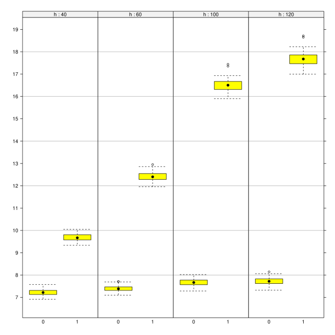
Figure 2: Boxplots of the estimates $\widehat{V}_{0}$ ($0$) and $\widetilde{V}_{0}$ ($1$) for different values of the bandwidth $h$.

In Figure 2 we show the boxplots of $\widetilde{V}_{0}$ and $\widehat{V}_{0}$ based on $100$ sets of trajectories each of the size $M=4000$ ($N=4000$) for different values of the bandwidth $h$, where the triangle kernel $K(x)=(1-\|x\|^{2})^{+}$ is used to construct (3.18). The true value $V_{0}$ of the option (computed using a two-dimensional binomial lattice) is $8.08$ in this case. Several observations can be made by an examination of Figure 2. First, while the bias of $\widehat{V}_{0}$ is always smaller then the bias of $\widetilde{V}_{0}$, the largest difference takes place for large $h$. This can be explained by the fact that for large $h$ more observations $Y^{(m)}_{r+1}$ with $X^{(m)}(t_{r})$ lying far away from the given point $x$ become involved in the construction of $\widehat{C}_{r,M}(x)$. This has a consequence of increasing the bias of the estimate (3.18) and $\widetilde{V}_{0}$ quickly deteriorates with increasing $h$ . The most interesting phenomenon is, however, the behavior of $\widehat{V}_{0}$ which turns out to be quite stable with respect to $h$. So, in the case of rather poor estimates of continuation values (when $h$ is increases) $\widehat{V}_{0}$ looks very reasonable and even becomes closer to the true price.

We stress that the aim of this example is not to show the strength of the local polynomial estimation algorithms (although the performance of $\widehat{V}_{0}$ for $h=120$ is quite comparable to the performance of a linear regression algorithm reported in Glasserman (2004)) but rather to illustrate the main message of this paper, namely the message about the efficiency of $\widehat{V}_{0}$ as compared to the estimates based on the direct use of continuation values estimates.

4 Conclusion

In this paper we derive optimal rates of convergence for low biased estimates for the price of a Bermudan option based on suboptimal exercise policies obtained from some estimates of the optimal continuation values. We have shown that these rates are usually much faster than the convergence rates of the corresponding continuation values estimates. This may explain the efficiency of these lower bounds observed in practice. Moreover, it turns out that there are some cases where the expected values of the lower bounds based on suboptimal stopping rules achieve very fast convergence rates which are exponential in the number of paths used to estimate the corresponding continuation values.

5 Proofs

5.1 Proof of Proposition 2.1

Define

$$\tau_{j} := \min\{j\leq k<L:C_{k}(X(t_{k}))\leq f_{k}(X(t_{k}))\},\quad j=0,\ldots,L,$$

$$\widehat{\tau}_{j,M} := \min\{j\leq k<L:\widehat{C}_{k}(X(t_{k}))\leq f_{k}(X(t_{k}))\},\quad j=0,\ldots,L$$

and

$$V_{k,M}(x):=\operatorname{E}[f_{\widehat{\tau}_{k,M}}(X(t_{\widehat{\tau}_{k,M}}))|X(t_{k})=x],\quad x\in\mathbb{R}^{d}.$$

The so called Snell envelope process $V_{k}$ is related to $\tau_{k}$ via

$$V_{k}(x)=\operatorname{E}[f_{\tau_{k}}(X(t_{\tau_{k}}))|X(t_{k})=x],\quad x\in\mathbb{R}^{d}.$$

The following lemma provides a useful inequality which will be repeatedly used in our analysis.

Lemma 5.1.

For any $k=0,\ldots,L-1$, it holds with probability one

(5.19) $$0\leq V_{k}(X(t_{k}))-V_{k,M}(X(t_{k}))\\ \leq\operatorname{E}^{\mathcal{F}_{t_{k}}}\left[\sum_{l=k}^{L-1}|f_{l}(X(t_{l}))-C_{l}(X(t_{l}))|\right.\\ \left.\times\left(\mathbf{1}_{\{\widehat{\tau}_{l,M}>l,\,\tau_{l}=l\}}+\mathbf{1}_{\{\widehat{\tau}_{l,M}=l,\,\tau_{l}>l\}}\right)\right].$$

Proof.

We shall use induction to prove (5.19). For $k=L-1$ we have

(5.20) $$V_{L-1}(X(t_{L-1}))-V_{L-1,M}(X(t_{L-1}))=\\ =\operatorname{E}^{\mathcal{F}_{t_{L-1}}}\left[(f_{L-1}(X(t_{L-1}))-f_{L}(X(t_{L})))\mathbf{1}_{\{\tau_{L-1}=L-1,\,\widehat{\tau}_{L-1,M}=L\}}\right]\\ +\operatorname{E}^{\mathcal{F}_{t_{L-1}}}\left[(f_{L}(X(t_{L}))-f_{L-1}(X(t_{L-1})))\mathbf{1}_{\{\tau_{L-1}=L,\,\widehat{\tau}_{L-1,M}=L-1\}}\right]\\ =|f_{L-1}(X(t_{L-1}))-C_{L-1}(X(t_{L-1}))|\mathbf{1}_{\{\widehat{\tau}_{L-1,M}\neq\tau_{L-1}\}}$$

since events $\{\tau_{L-1}=L\}$ and $\{\widehat{\tau}_{L-1,M}=L\}$ are measurable w.r.t. $\mathcal{F}_{t_{L-1}}$. Thus, (5.19) holds with $k=L-1$. Suppose that (5.19) holds with $k=L^{\prime}+1$. Let us prove it for $k=L^{\prime}$. Consider a decomposition

$$f_{\tau_{L^{\prime}}}(X(t_{\tau_{L^{\prime}}}))-f_{\widehat{\tau}_{L^{\prime},M}}(X(t_{\widehat{\tau}_{L^{\prime},M}})) = S_{1}+S_{2}+S_{3}$$

with

$$S_{1} := \left(f_{\tau_{L^{\prime}}}(X(t_{\tau_{L^{\prime}}}))-f_{\widehat{\tau}_{L^{\prime},M}}(X(t_{\widehat{\tau}_{L^{\prime},M}}))\right)\mathbf{1}_{\{\tau_{L^{\prime}}>L^{\prime},\,\widehat{\tau}_{L^{\prime},M}>L^{\prime}\}}$$

$$S_{2} := \left(f_{\tau_{L^{\prime}}}(X(t_{\tau_{L^{\prime}}}))-f_{\widehat{\tau}_{L^{\prime},M}}(X(t_{\widehat{\tau}_{L^{\prime},M}}))\right)\mathbf{1}_{\{\tau_{L^{\prime}}>L^{\prime},\,\widehat{\tau}_{L^{\prime},M}=L^{\prime}\}}$$

$$S_{3} := \left(f_{\tau_{L^{\prime}}}(X(t_{\tau_{L^{\prime}}}))-f_{\widehat{\tau}_{L^{\prime},M}}(X(t_{\widehat{\tau}_{L^{\prime},M}}))\right)\mathbf{1}_{\{\tau_{L^{\prime}}=L^{\prime},\,\widehat{\tau}_{L^{\prime},M}>L^{\prime}\}}.$$

Since

$$\operatorname{E}^{\mathcal{F}_{t_{L^{\prime}}}}\left[S_{1}\right] = \operatorname{E}^{\mathcal{F}_{t_{L^{\prime}}}}\left[\left(V_{L^{\prime}+1}(X(t_{L^{\prime}+1}))-V_{L^{\prime}+1,M}(X(t_{L^{\prime}+1}))\right)\right]\mathbf{1}_{\{\tau_{L^{\prime}}>L^{\prime},\,\widehat{\tau}_{L^{\prime},M}>L^{\prime}\}},$$

$$\operatorname{E}^{\mathcal{F}_{t_{L^{\prime}}}}\left[S_{2}\right] = \left(\operatorname{E}^{\mathcal{F}_{t_{L^{\prime}}}}\left[f_{\tau_{L^{\prime}+1}}(X(t_{\tau_{L^{\prime}+1}}))\right]-f_{L^{\prime}}(X(t_{L^{\prime}}))\right)\mathbf{1}_{\{\tau_{L^{\prime}}>L^{\prime},\,\widehat{\tau}_{L^{\prime},M}=L^{\prime}\}}$$

$$= \left(C_{L^{\prime}}(X(t_{L^{\prime}}))-f_{L^{\prime}}(X(t_{L^{\prime}}))\right)\mathbf{1}_{\{\tau_{L^{\prime}}>L^{\prime},\,\widehat{\tau}_{L^{\prime},M}=L^{\prime}\}}$$

and

$$\operatorname{E}^{\mathcal{F}_{t_{L^{\prime}}}}\left[S_{3}\right] = \left(f_{L^{\prime}}(X(t_{L^{\prime}}))-\operatorname{E}^{\mathcal{F}_{t_{L^{\prime}}}}\left[f_{\widehat{\tau}_{L^{\prime}+1,M}}(X(t_{\widehat{\tau}_{L^{\prime}+1,M}}))\right]\right)\mathbf{1}_{\{\tau_{L^{\prime}}=L^{\prime},\,\widehat{\tau}_{L^{\prime},M}>L^{\prime}\}}$$

$$= \left(f_{L^{\prime}}(X(t_{L^{\prime}}))-C_{L^{\prime}}(X(t_{L^{\prime}}))\right)\mathbf{1}_{\{\tau_{L^{\prime}}=L^{\prime},\,\widehat{\tau}_{L^{\prime},M}>L^{\prime}\}}$$

$$+\operatorname{E}^{\mathcal{F}_{t_{L^{\prime}}}}\left[\left(V_{L^{\prime}+1}(X(t_{L^{\prime}+1}))-V_{L^{\prime}+1,M}(X(t_{L^{\prime}+1}))\right)\mathbf{1}_{\{\tau_{L^{\prime}}=L^{\prime},\,\widehat{\tau}_{L^{\prime},M}>L^{\prime}\}}\right],$$

we get with probability one

$$V_{L^{\prime}}(X(t_{L^{\prime}}))-V_{L^{\prime},M}(X(t_{L^{\prime}}) \leq \left|f_{L^{\prime}}(X(t_{L^{\prime}}))-C_{L^{\prime}}(X(t_{L^{\prime}}))\right|$$

$$\times\left(\mathbf{1}_{\{\widehat{\tau}_{L^{\prime},M}>L^{\prime},\,\tau_{L^{\prime}}=L^{\prime}\}}+\mathbf{1}_{\{\widehat{\tau}_{L^{\prime},M}=L^{\prime},\,\tau_{L^{\prime}}>L^{\prime}\}}\right)$$

$$+\operatorname{E}^{\mathcal{F}_{t_{L^{\prime}}}}\left[V_{L^{\prime}+1}(X(t_{L^{\prime}+1}))-V_{L^{\prime}+1,M}(X(t_{L^{\prime}+1}))\right].$$

Our induction assumption implies now that

$$V_{L^{\prime}}(X(t_{L^{\prime}}))-V_{L^{\prime},M}(X(t_{L^{\prime}}))\leq\\ \operatorname{E}^{\mathcal{F}_{t_{L^{\prime}}}}\left[\sum_{l=L^{\prime}}^{L-1}|f_{l}(X_{l})-C_{l}(X_{l})|\left(\mathbf{1}_{\{\widehat{\tau}_{l,M}>l,\,\tau_{l}=l\}}+\mathbf{1}_{\{\widehat{\tau}_{l,M}=l,\,\tau_{l}>l\}}\right)\right]$$

and hence (5.19) holds for $k=L^{\prime}$. ∎

Let us continue with the proof of Proposition 2.1. Consider the sets $\mathcal{E}_{l},\,\mathcal{A}_{l,j}\subset\mathbb{R}^{d},\,l=0,\ldots,L-1,\,j=1,2,\ldots,$ defined as

$$\mathcal{E}_{l} := \left\{x\in\mathbb{R}^{d}:\widehat{C}_{l,M}(x)\leq f_{l}(x),\,C_{l}(x)>f_{l}(x)\right\}$$

$$\cup\left\{x\in\mathbb{R}^{d}:\widehat{C}_{l,M}(x)>f_{l}(x),\,C_{l}(x)\leq f_{l}(x)\right\},$$

$$\mathcal{A}_{l,0} := \left\{x\in\mathbb{R}^{d}:0<\left|C_{l}(x)-f_{l}(x)\right|\leq\gamma^{-1/2}_{M}\right\},$$

$$\mathcal{A}_{l,j} := \left\{x\in\mathbb{R}^{d}:2^{j-1}\gamma^{-1/2}_{M}<\left|C_{l}(x)-f_{l}(x)\right|\leq 2^{j}\gamma^{-1/2}_{M}\right\},\quad j>0.$$

We may write

$$V_{0}(X(t_{0}))-V_{0,M}(X(t_{0})) \leq \operatorname{E}^{\mathcal{F}_{t_{0}}}\left[\sum_{l=0}^{L-1}|f_{l}(X(t_{l}))-C_{l}(X(t_{l}))|\mathbf{1}_{\{X(t_{l})\in\mathcal{E}_{l}\}}\right]$$

$$= \sum_{j=0}^{\infty}\operatorname{E}^{\mathcal{F}_{t_{0}}}\left[\sum_{l=0}^{L-1}|f_{l}(X(t_{l}))-C_{l}(X(t_{l}))|\mathbf{1}_{\{X(t_{l})\in\mathcal{A}_{l,j}\cap\mathcal{E}_{l}\}}\right]$$

$$\leq \gamma_{M}^{-1/2}\sum_{l=0}^{L-1}\operatorname{P}_{t_{l}|t_{0}}\left(0<\left|C_{l}(X(t_{l}))-f_{l}(X(t_{l}))\right|\leq\gamma_{M}^{-1/2}\right)$$

$$+\sum_{j=1}^{\infty}\operatorname{E}^{\mathcal{F}_{t_{0}}}\left[\sum_{l=0}^{L-1}|f_{l}(X(t_{l}))-C_{l}(X(t_{l}))|\mathbf{1}_{\{X(t_{l})\in\mathcal{A}_{l,j}\cap\mathcal{E}_{l}\}}\right].$$

Using the fact that

$$|f_{l}(X(t_{l}))-C_{l}(X(t_{l}))|\leq|\widehat{C}_{l,M}(X(t_{l})-C_{l}(X(t_{l}))|,\quad l=0,\ldots,L-1,$$

on $\mathcal{E}_{l}$, we get for any $j\geq 1$ and $l\geq 0$

$$\operatorname{E}^{\mathcal{F}_{t_{0}}}\operatorname{E}_{\operatorname{P}_{x_{0}}^{\otimes M}}\left[|f_{l}(X(t_{l}))-C_{l}(X(t_{l}))|\mathbf{1}_{\{X(t_{l})\in\mathcal{A}_{l,j}\cap\mathcal{E}_{l}\}}\right]\\ \leq 2^{j}\gamma_{M}^{-1/2}\operatorname{E}^{\mathcal{F}_{t_{0}}}\operatorname{E}_{\operatorname{P}_{x_{0}}^{\otimes M}}\left[\mathbf{1}_{\{|\widehat{C}_{l,M}(X(t_{l})-C_{l}(X(t_{l}))|\geq 2^{j-1}\gamma_{M}^{-1/2}\}}\right.\\ \left.\times\mathbf{1}_{\{0<|f_{l}(X(t_{l}))-C_{l}(X(t_{l}))|\leq 2^{j}\gamma_{M}^{-1/2}\}}\right]\\ \leq 2^{j}\gamma_{M}^{-1/2}\operatorname{E}^{\mathcal{F}_{t_{0}}}\left[\operatorname{P}_{x_{0}}^{\otimes M}(|\widehat{C}_{l,M}(X(t_{l}))-C_{l}(X(t_{l}))|\geq 2^{j-1}\gamma_{M}^{-1/2})\right.\\ \left.\times\mathbf{1}_{\{0<|f_{l}(X(t_{l}))-C_{l}(X(t_{l}))|\leq 2^{j}\gamma_{M}^{-1/2}\}}\right]\\ \leq B_{1}2^{j}\gamma_{M}^{-1/2}\exp\left(-B_{2}2^{j-1}\right)\operatorname{P}_{t_{l}|t_{0}}(0<|f_{l}(X(t_{l}))-C_{l}(X(t_{l}))|\leq 2^{j}\gamma_{M}^{-1/2})\\ \leq B_{1}B_{0,l}2^{j(1+\alpha)}\gamma_{M}^{-(1+\alpha)/2}\exp\left(-B_{2}2^{j-1}\right),$$

where Assumption 2.3 is used to get the last inequality. Finally, we get

$$V_{0}(X(t_{0}))-\operatorname{E}_{\operatorname{P}_{x_{0}}^{\otimes M}}\left[V_{0,M}(X(t_{0}))\right]\\ \leq\left[\sum_{l=0}^{L-1}B_{0,l}\right]\gamma_{M}^{-(1+\alpha)/2}+B^{\prime}\left[\sum_{l=0}^{L-1}B_{0,l}\right]\gamma_{M}^{-(1+\alpha)/2}\sum_{j\geq 1}2^{j(1+\alpha)}\exp(-B_{2}2^{j-1})\\ \leq B\left[\sum_{l=0}^{L-1}B_{0,l}\right]\gamma_{M}^{-(1+\alpha)/2}$$

with some constant $B$ depending on $B_{1}$, $B_{2}$ and $\alpha.$

5.2 Proof of Proposition 2.2

We have

(5.21) $$V_{0}(X(t_{0}))-\widehat{V}_{0,M}(X(t_{0}))=\\ =\operatorname{E}^{\mathcal{F}_{t_{0}}}\left[(f_{1}(X(t_{1}))-f_{2}(X(t_{2})))1(\tau_{1}=1,\widehat{\tau}_{1,M}=2)\right]\\ +\operatorname{E}^{\mathcal{F}_{t_{0}}}\left[(f_{2}(X(t_{2}))-f_{1}(X(t_{1})))1(\tau_{1}=2,\widehat{\tau}_{1,M}=1)\right]\\ =\operatorname{E}^{\mathcal{F}_{t_{0}}}\left[|f_{1}(X(t_{1}))-C_{1}(X(t_{1}))|\mathbf{1}_{\{\widehat{\tau}_{1,M}\neq\tau_{1}\}}\right].$$

For an integer $q\geq 1$ consider a regular grid on $[0,1]^{d}$ defined as

$$G_{q}=\left\{\left(\frac{2k_{1}+1}{2q},\ldots,\frac{2k_{d}+1}{2q}\right):\,k_{i}\in\{0,\ldots,q-1\},\,i=1,\ldots,d\right\}.$$

Let $n_{q}(x)\in G_{q}$ be the closest point to $x\in\mathbb{R}^{d}$ among points in $G_{q}$. Consider the partition $\mathcal{X}^{\prime}_{1},\ldots,\mathcal{X}^{\prime}_{q^{d}}$ of $[0,1]^{d}$ canonically defined using the grid $G_{q}$ ($x$ and $y$ belong to the same subset if and only if $n_{q}(x)=n_{q}(y)$). Fix an integer $m\leq q^{d}$. For any $i\in\{1,\ldots,m\}$, define $\mathcal{X}_{i}=\mathcal{X}^{\prime}_{i}$ and $\mathcal{X}_{0}=\mathbb{R}^{d}\setminus\bigcup_{i=1}^{m}\mathcal{X}_{i}$, so that $\mathcal{X}_{0},\ldots,\mathcal{X}_{m}$ form a partition of $\mathbb{R}^{d}$. Denote by $\mathcal{B}_{q,j}$ the ball with the center in $n_{q}(\mathcal{X}_{j})$ and radius $1/2q$.

Define a hypercube $\mathcal{H}=\{P_{\bar{\sigma}}:\bar{\sigma}=(\sigma_{1},\ldots,\sigma_{m})\in\{-1,1\}^{m}\}$ of probability distributions $\operatorname{P}_{\bar{\sigma}}$ of the r.v. $(X(t_{1}),f_{2}(X(t_{2})))$ valued in $\mathbb{R}^{d}\times\{0,1\}$ as follows. For any $\operatorname{P}_{\bar{\sigma}}\in\mathcal{H}$ the marginal distribution of $X(t_{1})$ (given $X(t_{0})=x_{0}$) does not depend on $\bar{\sigma}$ and has a bounded density $\mu$ w.r.t. the Lebesgue measure on $\mathbb{R}^{d}$ such that $\operatorname{P}_{\mu}(\mathcal{X}_{0})=0$ and

$$\operatorname{P}_{\mu}(\mathcal{X}_{j})=\operatorname{P}_{\mu}(\mathcal{B}_{q,j})=\int_{\mathcal{B}_{q,j}}\mu(x)\,dx=\omega,\quad j=1,\ldots,m$$

for some $\omega>0$. In order to ensure that the density $\mu$ remains bounded we assume that $q^{d}\omega=O(1)$.

The distribution of $f_{2}(X(t_{2}))$ given $X(t_{1})$ is determined by the probability $\operatorname{P}_{\bar{\sigma}}(f_{2}(X(t_{2}))=1|X(t_{1})=x)$ which is equal to $C_{1,\bar{\sigma}}(x)$. Define

$$C_{1,\bar{\sigma}}(x)=f_{1}(x)+\sigma_{j}\phi(x),\quad x\in\mathcal{X}_{j},\quad j=1,\ldots,m,$$

and $C_{1,\bar{\sigma}}(x)=f_{1}(x)$ on $\mathcal{X}_{0}$, where $\phi(x)=\gamma^{-1/2}_{M}\varphi(q[x-n_{q}(x)])$, $\varphi(x)=A_{\varphi}\theta(\|x\|)$ with some constant $A_{\varphi}>0$ and with $\theta:\mathbb{R}_{+}\to\mathbb{R}_{+}$ being a non-increasing infinitely differentiable function such that $\theta(x)\equiv 1$ on $[0,1/2]$ and $\theta(x)\equiv 0$ on $[1,\infty)$. Furthermore, there exist two real numbers $0<f_{-}<f_{+}<1$ such that $f_{-}\leq f_{1}(x)\leq f_{+}.$ Taking $A_{\varphi}$ small enough, we can then ensure that $0\leq C_{1,\bar{\sigma}}(x)\leq 1$ on $\mathbb{R}^{d}$. Obviously, it holds $\phi(x)=A_{\varphi}\gamma^{-1/2}_{M}$ for $x\in\mathcal{B}_{q,j}$. As to the boundary assumption (2.3), we have

$$\operatorname{P}_{\mu}(0<|f_{1}(X(t_{1}))-C_{1,\bar{\sigma}}(X(t_{1}))|\leq\delta)=\\ \sum_{j=1}^{m}\operatorname{P}_{\mu}(0<|f_{1}(X(t_{1}))-C_{1,\bar{\sigma}}(X(t_{1}))|\leq\delta,X(t_{1})\in\mathcal{B}_{q,j})\\ =\sum_{j=1}^{m}\int_{\mathcal{B}_{q,j}}\mathbf{1}_{\{0<\phi(x)\leq\delta\}}\mu(x)\,dx=m\omega\mathbf{1}_{\{A_{\varphi}\gamma_{M}^{-1/2}\leq\delta\}}$$

and (2.3) holds provided that $m\omega=O(\gamma^{-\alpha/2}_{M})$. Let $\widehat{\tau}_{M}$ be a stopping time measurable w.r.t. $\mathcal{F}^{\otimes M}$, then the identity (5.21) leads to

$$\operatorname{E}^{\mathcal{F}_{t_{0}}}_{\operatorname{P}_{\bar{\sigma}}}[f_{\tau}(X(\tau))]-\operatorname{E}_{\operatorname{P}_{\bar{\sigma}}^{\otimes M}}[\operatorname{E}^{\mathcal{F}_{t_{0}}}f_{\widehat{\tau}_{M}}(X(\widehat{\tau}_{M}))]\\ =\operatorname{E}_{\operatorname{P}_{\bar{\sigma}}^{\otimes M}}\operatorname{E}_{P_{\mu}}^{\mathcal{F}_{t_{0}}}\left[|\Delta_{\bar{\sigma}}(X(t_{1}))|\mathbf{1}_{\{\widehat{\tau}_{1,M}\neq\tau_{1}\}}\right],$$

with $\Delta_{\bar{\sigma}}(X(t_{1}))=f_{1}(X(t_{1}))-C_{1,\bar{\sigma}}(X(t_{1}))$. By conditioning on $X(t_{1}),$ we get

$$\operatorname{E}_{\operatorname{P}_{\bar{\sigma}}^{\otimes M}}\operatorname{E}_{\operatorname{P}_{\mu}}^{\mathcal{F}_{t_{0}}}\left[|\Delta_{\bar{\sigma}}(X(t_{1}))|\mathbf{1}_{\{\widehat{\tau}_{1,M}\neq\tau_{1}\}}\right]\\ =\omega\sum_{j=1}^{m}\operatorname{E}_{\operatorname{P}_{\bar{\sigma}}^{\otimes M}}\operatorname{E}_{\operatorname{P}_{\mu}}^{\mathcal{F}_{t_{0}}}\left[\phi(X(t_{1}))\mathbf{1}_{\{\widehat{\tau}_{1,M}\neq\tau_{1}\}}|X(t_{1})\in\mathcal{B}_{q,j}\right]\\ =A_{\varphi}m\omega\gamma_{M}^{-1/2}\operatorname{E}_{\operatorname{P}_{\mu}}^{\mathcal{F}_{t_{0}}}\operatorname{P}_{\bar{\sigma}}^{\otimes M}(\widehat{\tau}_{1,M}\neq\tau_{1}).$$

Using now a well known Birgé’s or Huber’s lemma (see, e.g. Devroye, Györfi and Lugosi, 1996, p. 243), we get

$$\sup_{\bar{\sigma}\in\{-1;+1\}^{m}}\operatorname{P}_{\bar{\sigma}}^{\otimes M}(\widehat{\tau}_{1,M}\neq\tau_{1})\geq\left[0.36\wedge\left(1-\frac{MK_{\mathcal{H}}}{\log(\mathcal{|H|})}\right)\right],$$

where $K_{\mathcal{H}}:=\sup_{P,Q\in\mathcal{H}}K(P,Q)$ and $K(P,Q)$ is a Kullback-Leibler distance between two measures $P$ and $Q$. Since for any two measures $P$ and $Q$ from $\mathcal{H}$ with $Q\neq P$ it holds

$$K(P,Q) \leq \sup_{\begin{subarray}{c}\bar{\sigma}_{1},\bar{\sigma}_{2}\in\{-1;+1\}^{m}\\ \bar{\sigma}_{1}\neq\bar{\sigma}_{2}\end{subarray}}\operatorname{E}_{\operatorname{P}_{\mu}}^{\mathcal{F}_{t_{0}}}\left[C_{1,\bar{\sigma}_{2}}(X(t_{1}))\log\left\{\frac{C_{1,\bar{\sigma}_{1}}(X(t_{1}))}{C_{1,\bar{\sigma}_{2}}(X(t_{1}))}\right\}\right.$$

$$\left.+(1-C_{1,\bar{\sigma}_{2}}(X(t_{1})))\log\left\{\frac{1-C_{1,\bar{\sigma}_{1}}(X(t_{1}))}{1-C_{1,\bar{\sigma}_{2}}(X(t_{1}))}\right\}\right]$$

$$\leq (1-f_{+}-A_{\varphi})^{-1}(f_{-}-A_{\varphi})^{-1}\operatorname{E}_{\operatorname{P}_{\mu}}^{\mathcal{F}_{t_{0}}}\left[\phi^{2}(X(t_{1}))\mathbf{1}_{\{X(t_{1})\not\in\mathcal{X}_{0}\}}\right]$$

for small enough $A_{\varphi}$, and $\log(|\mathcal{H}|)=m\log(2)$, we get

$$\sup_{\bar{\sigma}\in\{-1;+1\}^{m}}\left\{\operatorname{E}^{\mathcal{F}_{t_{0}}}_{\operatorname{P}_{\bar{\sigma}}}[f_{\tau,\bar{\sigma}}(X(\tau))]-\operatorname{E}_{\operatorname{P}_{\bar{\sigma}}^{\otimes M}}[\operatorname{E}^{\mathcal{F}_{t_{0}}}f_{\widehat{\tau}_{M},\bar{\sigma}}(X(\widehat{\tau}_{M}))]\right\}\geq\\ A_{\varphi}m\omega\gamma^{-1/2}_{M}(1-AM\gamma^{-1}_{M}\omega)\gtrsim\gamma_{M}^{-(1+\alpha)/2},$$

provided that $m\omega>B\gamma^{-\alpha/2}_{M}$ for some $B>0$ and $AM\omega<\gamma_{M},$ where $A$ is a positive constant depending on $f_{-},f_{+}$ and $A_{\varphi}.$ Using similar arguments, we derive

$$\sup_{\bar{\sigma}\in\{-1;+1\}^{m}}\operatorname{P}_{\bar{\sigma}}^{\otimes M}(|C_{1,\bar{\sigma}}(x)-\widehat{C}_{1,M}(x)|>\delta\gamma_{M}^{-1/2})>0$$

for almost $x$ w.r.t. $\operatorname{P}_{\mu}$, some $\delta>0$ and any estimator $\widehat{C}_{1,M}$ measurable w.r.t. $\mathcal{F}^{\otimes M}$.

5.3 Proof of Proposition 2.3

Using the arguments similar to ones in the proof of Proposition 2.1, we get

(5.22) $$V_{0}(X(t_{0}))-\operatorname{E}_{\operatorname{P}_{x_{0}}^{\otimes M}}\left[V_{0,M}(X(t_{0}))\right]\leq\\ \delta_{0}\sum_{l=0}^{L-1}\operatorname{P}_{t_{l}|t_{0}}(0<|C_{l}(X(t_{l}))-f_{l}(X(t_{l}))|\leq\delta_{0})\\ +\sum_{l=0}^{L-1}\operatorname{E}^{\mathcal{F}_{t_{0}}}\operatorname{E}_{\operatorname{P}_{x_{0}}^{\otimes M}}\left[|C_{l}(X(t_{l}))-f_{l}(X(t_{l}))|\right.\\ \left.\times\mathbf{1}_{\{X(t_{l})\in\mathcal{E}_{l}\}}\mathbf{1}_{\{|C_{l}(X(t_{l}))-f_{l}(X(t_{l}))|>\delta_{0}\}}\right]$$

with $\mathcal{E}_{l}$ defined as in the proof of Proposition 2.1. The first summand on the right-hand side of (5.22) is equal to zero due to (2.8). Hence, Cauchy-Schwarz and Minkowski inequalities imply

$$V_{0}(X(t_{0}))-\operatorname{E}_{\operatorname{P}_{x_{0}}^{\otimes M}}\left[V_{0,M}(X(t_{0}))\right] \leq \sum_{l=0}^{L-1}\left[\operatorname{E}^{\mathcal{F}_{t_{0}}}|\operatorname{E}^{\mathcal{F}_{t_{l}}}\left[f_{\tau_{l+1}}(X(t_{\tau_{l+1}}))\right]-f_{l}(X(t_{l}))|^{2}\right]^{1/2}$$

$$\times\left[\operatorname{E}^{\mathcal{F}_{t_{0}}}\operatorname{P}_{x_{0}}^{\otimes M}(|C_{l}(X(t_{l}))-\widehat{C}_{l,M}(X(t_{l}))|>\delta_{0})\right]^{1/2}$$

$$\leq 2B^{1/2}_{f}\sum_{l=0}^{L-1}\left[\operatorname{E}^{\mathcal{F}_{t_{0}}}\operatorname{P}_{x_{0}}^{\otimes M}(|C_{l}(X(t_{l}))-\widehat{C}_{l,M}(X(t_{l}))|>\delta_{0})\right]^{1/2}.$$

Now the application of (2.9) finishes the proof.

5.4 Proof of Proposition 2.8

Denote

$$\varepsilon_{k,M}(x)=T[\widehat{C}_{k,M}](x)-C_{k}(x)$$

and

$$\zeta_{k,M}(x)=\widetilde{C}_{k,M}(x)-T[\widehat{C}_{k,M}](x)$$

for $k=1,\ldots,L-1$. Using the elementary inequality $|\max(a,x)-\max(a,y)|\leq|x-y|,$ which holds for any real numbers $a$, $x$ and $y$, we get

$$|\varepsilon_{k,M}(x)|\leq|\zeta_{k,M}(x)|+\operatorname{E}\left[\left.|\varepsilon_{k+1,M}(X(t_{k+1}))|\right|X(t_{k})=x\right]$$

and hence

$$|\varepsilon_{k,M}(x)| \leq \sum_{l=k+1}^{L-1}\operatorname{E}\left[|\zeta_{l,M}(X(t_{l}))||X(t_{k})=x\right]$$

$$:= \sum_{l=k+1}^{L-1}\xi_{l,k,M}(x).$$

Note that we take expectation in (5.4) with respect to a new $\sigma$-algebra $\mathcal{F}$ which is independent of $\mathcal{F}^{\otimes M}$ and $\{\zeta_{l,M}\}$ are measurable w.r.t $\mathcal{F}^{\otimes M}$. Hence, random variables $\{\xi_{l,k,M}\}$ are $\mathcal{F}^{\otimes M}$ measurable as well. According to Lemma 5.2 (see below)

$$\operatorname{P}^{\otimes M}_{x_{0}}\left(\xi_{l,k,M}(x)\geq\delta\sqrt{|\log h|/Mh^{d+2\nu}}\right)\leq\\ \operatorname{P}_{x_{0}}^{\otimes M}\left(\sup_{y\in\mathcal{A}}|\zeta_{l,M}(y)|\geq\delta\sqrt{|\log h|/Mh^{d+2\nu}}\right)\leq D_{2}\exp(-D_{3}\delta)$$

for almost all $x$ w.r.t. $\operatorname{P}_{t_{k}|t_{0}}$. Thus,

$$\operatorname{P}_{x_{0}}^{\otimes M}\left(|\varepsilon_{k,M}(x)|\geq\delta\sqrt{|\log h|/Mh^{d+2\nu}}\right)\leq LD_{2}\exp(-D_{3}\delta/L).$$

Analogously, using Lemma 5.3 one can prove that

$$\operatorname{P}_{x_{0}}^{\otimes M}\left(|\varepsilon_{k,M}(x)|\geq\delta\right)\leq B_{4}\exp(-B_{5}Mh^{d+\nu})$$

with some positive constants $B_{4}$ and $B_{5}.$

Lemma 5.2.

Let assumptions (AX0)-(AX2), (AK1) and (AK2) be fulfilled. Then there exist positive constants $D_{1}$, $D_{2}$ and $D_{3}$, such that for any $h$ satisfying $D_{1}h^{\beta}<\sqrt{|\log h|/Mh^{d}}$ the estimates $\{T[\widehat{C}_{k,M}]\}$ based on the truncated local polynomials estimators of degree $\lfloor\beta\rfloor$ fulfill

$$\operatorname{P}_{x_{0}}^{\otimes M}\left(\sup_{x\in\mathcal{A}}|T[\widehat{C}_{k,M}](x)-\widetilde{C}_{k}(x)|\geq\delta\sqrt{|\log h|/Mh^{d+2\nu}}\right)\leq D_{2}\exp(-D_{3}\delta),$$

for all $\delta>\delta_{0}$ and $k=1,\ldots,L-1$.

Lemma 5.3.

Let assumptions (AX0)-(AX2), (AK1) and (AK2) be fulfilled and $\sqrt{|\log h|/Mh^{d+2\nu}}=o(1)$ for $M\to\infty.$ Then there exist positive constants $D_{4}$, $D_{5}$ and $D_{6}$ such that for any $\delta\geq D_{4}h^{\beta}$ the inequality

$$\operatorname{P}_{x_{0}}^{\otimes M}\left(\sup_{x\in\mathcal{A}}|T[\widehat{C}_{k,M}](x)-\widetilde{C}_{k}(x)|\geq\delta\right)\leq D_{5}\exp(-D_{6}Mh^{d+\nu})$$

holds for all $k=1,\ldots,L-1$.

Proof.

We give the proof only for Lemma 5.2. Lemma 5.3 can be proved in a similar way. Fix some natural $r>0$ such that $0<r\leq L$ and consider the matrix $\Gamma=(\Gamma_{u_{1},u_{2}})_{|u_{1}|,|u_{2}|\leq\lfloor\beta\rfloor}$ with elements

$$\Gamma_{u_{1},u_{2}}=\frac{1}{Mh^{d}}\sum_{m=1}^{M}\left(\frac{X^{(m)}(t_{r})-x}{h}\right)^{u_{1}+u_{2}}K\left(\frac{X^{(m)}(t_{r})-x}{h}\right).$$

The smallest eigenvalue $\lambda_{\Gamma}$ of the matrix $\Gamma$ satisfies

(5.24) $$\lambda_{\Gamma} = \min_{\|W\|=1}W^{\top}\Gamma W$$

$$\geq \min_{\|W\|=1}W^{\top}\operatorname{E}[\Gamma]W+\min_{\|W\|=1}W^{\top}(\Gamma-\operatorname{E}[\Gamma])W$$

$$\geq \min_{\|W\|=1}W^{\top}\operatorname{E}[\Gamma]W-\sum_{|u_{1}|,|u_{2}|\leq\lfloor\beta\rfloor}|\Gamma_{u_{1},u_{2}}-\operatorname{E}[\Gamma_{u_{1},u_{2}}]|.$$

By Assumption (AX2)

$$\inf_{x\in\mathcal{A}}\min_{\|W\|=1}\left[W^{\top}\operatorname{E}[\Gamma(x)]W\right]\geq\gamma_{0}h^{\nu}$$

with some $\gamma_{0}>0.$ For $m=1,\ldots,M,$ and any multi-indices $u_{1}$, $u_{2}$ such that $|u_{1}|,|u_{2}|\leq\lfloor\beta\rfloor$, define

$$\Delta_{m}(x)=\frac{1}{h^{d}}\left(\frac{X^{(m)}(t_{r})-x}{h}\right)^{u_{1}+u_{2}}K\left(\frac{X^{(m)}(t_{r})-x}{h}\right)\\ -\int_{\mathbb{R}^{d}}z^{u_{1}+u_{2}}K(z)p(t_{r},x+hz|t_{0},x_{0})\,dz.$$

We have $\operatorname{E}_{\operatorname{P}_{t_{r}|t_{0}}}[\Delta_{m}(x)]=0$,

$$|\Delta_{m}(x)|\leq h^{-d}\sup_{z\in\mathbb{R}^{d}}\left[(1+\|z\|^{2\beta})K(z)\right]=:K_{1}h^{-d}$$

and

$$\operatorname{E}_{\operatorname{P}_{t_{r}|t_{0}}}[\Delta_{m}(x)]^{2} \leq \int_{\mathbb{R}^{d}}z^{2u_{1}+2u_{2}}K^{2}(z)p(t_{r},x+hz|t_{0},x_{0})\,dz$$

$$\leq \frac{p_{\max}}{h^{d}}\int_{\mathbb{R}^{d}}(1+\|z\|^{4\beta})K^{2}(z)\,dz=:K_{2}h^{-d},$$

where $p_{\max}=\sup_{z\in\mathbb{R}^{d}}p(t_{r},z|t_{0},x_{0})$ and $K_{1},K_{2}$ are two positive constants. Due to assumption (AK2), the class of functions

$$\left\{\left(\frac{x-\cdot}{h}\right)^{u_{1}+u_{2}}K\left(\frac{x-\cdot}{h}\right):\,x\in\mathbb{R}^{d},\,h\in\mathbb{R}\setminus\{0\},\,|u_{1}|,|u_{2}|\leq\lfloor\beta\rfloor\right\}$$

is a bounded Vapnik-Červonenkis class of measurable functions (see Dudley (1999)). According to Proposition 6.1 (see Appendix), we have for any $\zeta>0$

(5.25) $$\operatorname{P}_{t_{r}|t_{0}}\left(\sup_{x\in\mathcal{A}}|\Gamma_{u_{1},u_{2}}(x)-\operatorname{E}\Gamma_{u_{1},u_{2}}(x)|\geq\zeta\right)\\ =\operatorname{P}_{t_{r}|t_{0}}\left(\sup_{x\in\mathcal{A}}\frac{1}{M}\left|\sum_{m=1}^{M}\Delta_{m}(x)\right|\geq\zeta\right)\\ \leq L_{0}\exp(-\zeta B_{0}Mh^{d})$$

with some positive constants $L_{0}$ and $B_{0}$. Combining (5.24) and ((AX2)) with (5.25), we get

$$\operatorname{P}_{t_{r}|t_{0}}\left(\inf_{x\in\mathcal{A}}\lambda_{\Gamma}(x)\leq\gamma_{0}h^{\nu}/2\right)\leq L_{0}N^{2}_{\beta}\exp(-\gamma_{0}B_{0}Mh^{d+\nu}/2N^{2}_{\beta}),$$

where $N^{2}_{\beta}$ is the number of elements in the matrix $\Gamma.$ Assume that $M$ is large enough so that $\gamma_{0}/2>(\log M)^{-1}.$ Then on the set $\{\inf_{x\in\mathcal{A}}\lambda_{\Gamma}(x)>\gamma_{0}h^{\nu}/2\}$ we have

$$|T[\widehat{C}_{r,M}](x)-\widetilde{C}_{r}(x)|\leq|\widehat{C}_{r,M}(x)-\widetilde{C}_{r}(x)|,\quad x\in\mathcal{A}$$

since $\sup_{x\in\mathcal{A}}\widetilde{C}_{r}(x)\leq C_{\max}.$ Therefore, it holds for any $\zeta>0$

$$\operatorname{P}_{t_{r}|t_{0}}\left(\sup_{x\in\mathcal{A}}|T[\widehat{C}_{r,M}](x)-\widetilde{C}_{r}(x)|\geq\zeta\right)\leq\operatorname{P}_{t_{r}|t_{0}}\left(\inf_{x\in\mathcal{A}}\lambda_{\Gamma}(x)\leq\gamma_{0}h^{\nu}/2\right)\\ +\operatorname{P}_{t_{r}|t_{0}}\left(\sup_{x\in\mathcal{A}}|\widehat{C}_{r,M}(x)-\widetilde{C}_{r}(x)|\geq\zeta,\,\inf_{x\in\mathcal{A}}\lambda_{\Gamma}(x)>\gamma_{0}h^{\nu}/2\right).$$

Introduce the matrix $Q=(Q_{m,u})_{1\leq m\leq M,\,|u|\leq\lfloor\beta\rfloor}$ with elements

$$Q_{m,u}=\left(\frac{X^{(m)}(t_{r})-x}{h}\right)^{u}\sqrt{\frac{1}{Mh^{d}}K\left(\frac{X^{(m)}(t_{r})-x}{h}\right)}.$$

Denote by $Q_{u}$ the $u$th column of $Q$ and define

$$Q^{C}(x):=\sum_{|u|\leq\lfloor\beta\rfloor}\frac{\widetilde{C}_{r}^{(u)}(x)h^{u}}{u!}Q_{u}.$$

Since $\Gamma=Q^{\top}Q$, we get $Z^{\top}(0)\Gamma^{-1}Q^{\top}Q_{u}=\mathbf{1}_{\{u=(0,\ldots,0)\}}$ for any $s$ with $|s|\leq\lfloor\beta\rfloor.$ Hence $Z^{\top}(0)\Gamma^{-1}Q^{\top}Q^{C}=\widetilde{C}_{r}(x)$. Thus, we can write

$$\widehat{C}_{r,M}(x)-\widetilde{C}_{r}(x)=Z^{\top}(0)\Gamma^{-1}(S-Q^{\top}Q^{C})=:Z^{\top}(0)\Gamma^{-1}\varepsilon_{M}(x),$$

where $\varepsilon_{M}(x)$ is a vector valued function with components

$$\varepsilon_{M,u}(x) = \frac{1}{Mh^{d}}\sum_{m=1}^{M}\left[Y_{r+1}^{(m)}-\widetilde{C}_{r,x}(X^{(m)}(t_{r}))\right]\left(\frac{X_{r}^{(m)}-x}{h}\right)^{u}K\left(\frac{X_{r}^{(m)}-x}{h}\right)$$

and $Y_{r+1}^{(m)}=\max(f_{r+1}(X^{(m)}(t_{r+1})),T[\widehat{C}_{r+1,M}](X^{(m)}(t_{r+1}))).$ So, on the set $\{\inf_{x\in\mathcal{A}}\lambda_{\Gamma}(x)>\gamma_{0}h^{\nu}/2\}$ we get

$$|\widehat{C}_{r,M}(x)-\widetilde{C}_{r}(x)|\leq\|\Gamma\varepsilon_{M}\|\leq\lambda_{\Gamma}^{-1}\|\varepsilon_{M}\|\leq 2h^{-\nu}\gamma_{0}^{-1}\|\varepsilon_{M}\|\leq 2h^{-\nu}\gamma_{0}^{-1}N^{1/2}_{\beta}\max_{u}|\varepsilon_{M,u}(x)|.$$

Denote

$$\Delta^{(1)}_{u,m}(x) := \frac{1}{h^{d}}\left[Y_{r+1}^{(m)}-\widetilde{C}_{r}(X^{(m)}(t_{r}))\right]\left(\frac{X_{r}^{(m)}-x}{h}\right)^{u}K\left(\frac{X_{r}^{(m)}-x}{h}\right),$$

$$\Delta^{(2)}_{u,m}(x) := \frac{1}{h^{d}}\left[\widetilde{C}_{r}(X^{(m)}(t_{r}))-\widetilde{C}_{r,x}(X^{(m)}(t_{r}))\right]\left(\frac{X_{r}^{(m)}-x}{h}\right)^{u}K\left(\frac{X_{r}^{(m)}-x}{h}\right).$$

It holds

$$|\varepsilon_{M,u}|\leq\left|\frac{1}{M}\sum_{m=1}^{M}\Delta_{u,m}^{(1)}\right|+\left|\frac{1}{M}\sum_{m=1}^{M}\left[\Delta_{u,m}^{(2)}-\operatorname{E}\Delta_{u,m}^{(2)}\right]\right|+|\operatorname{E}\Delta_{u,m}^{(2)}|.$$

Note that $\operatorname{E}_{\operatorname{P}_{t_{r}|t_{0}}}\left[\Delta_{u,m}^{(1)}\right]=0$ and

$$|\Delta_{u,m}^{(1)}(x)|\leq A_{11}h^{-d},\quad\operatorname{Var}\left[\Delta_{u,m}^{(1)}(x)\right]\leq A_{12}h^{-d},$$

$$\left|\Delta_{u,m}^{(2)}(x)-\operatorname{E}\left[\Delta_{u,m}^{(2)}(x)\right]\right|\leq A_{21}h^{\beta-d},\quad\operatorname{Var}\left[\Delta_{u,m}^{(2)}(x)\right]\leq A_{22}h^{2\beta-d}$$

with some positive constants $A_{11}$, $A_{12}$, $A_{21}$ and $A_{22}$ not depending on $x$. Proposition 6.1 implies that for any $\delta\geq\delta_{0}>0$

$$\operatorname{P}_{t_{r}|t_{0}}\left(\left\|\frac{1}{M}\sum_{m=1}^{M}\Delta_{u,m}^{(1)}\right\|_{\infty}\geq\delta\sqrt{|\log h|/Mh^{d}}\right)\leq L_{1}\exp\left(-\delta B_{1}|\log h|\right)$$

with some positive constants $L_{1}$ and $B_{1}$. Furthermore, due to the representation

$$\widetilde{C}_{r}(z)-\widetilde{C}_{r,x}(z)=\lfloor\beta\rfloor\sum_{|u|=\lfloor\beta\rfloor}\frac{(z-x)^{u}}{u!}\\ \times\int_{0}^{1}\left[\widetilde{C}^{(u)}_{r}(x+w(z-x))-\widetilde{C}^{(u)}_{r}(x)\right](1-w)^{\lfloor\beta\rfloor-1}\,dw$$

we get for any two points $x_{1}$ and $x_{2}$ in $\mathbb{R}^{d}$

$$\|\widetilde{C}_{r}(\cdot)-\widetilde{C}_{r,x_{1}}(\cdot)-(\widetilde{C}_{r}(\cdot)-\widetilde{C}_{r,x_{2}}(\cdot))\|_{\mathcal{A}}\leq\|x_{1}-x_{2}\|^{\beta-\lfloor\beta\rfloor}.$$

Now it can be shown (see Dudley (1999)) that the class

$$\left\{\left[\widetilde{C}_{r}(\cdot)-\widetilde{C}_{r,x}(\cdot)\right]\left(\frac{\cdot-x}{h}\right)^{u}K\left(\frac{\cdot-x}{h}\right):\,x\in\mathbb{R}^{d},\,h\in\mathbb{R}\setminus\{0\},\,|u|\leq\lfloor\beta\rfloor\right\}$$

is a bounded Vapnik-Červonenkis class of measurable functions. Hence

$$\operatorname{P}_{t_{r}|t_{0}}\left(\left\|\frac{1}{M}\sum_{m=1}^{M}\left[\Delta_{u,m}^{(2)}-\operatorname{E}_{\operatorname{P}_{t_{r}|t_{0}}}\Delta_{u,m}^{(2)}\right]\right\|_{\infty}\geq\delta\sqrt{|\log h|/Mh^{d}}\right)\leq L_{2}\exp\left(-\delta B_{2}|\log h|\right)$$

for $\delta\geq\delta_{0}>0$ and some positive constants $L_{2}$ and $B_{2}.$ Furthermore, using the inequality $|\operatorname{E}_{\operatorname{P}_{t_{r}|t_{0}}}[\Delta_{u,m}^{(2)}]|\leq A_{3}h^{\beta},$ we arrive at

$$\operatorname{P}_{t_{r}|t_{0}}\left(\sup_{x\in\mathcal{A}}|\varepsilon_{M,u}(x)|\geq\gamma_{0}\delta\sqrt{|\log h|/(Mh^{d}N_{\beta})}\right)\leq L_{3}\exp\left(-\delta B_{3}|\log h|\right)$$

with some positive constants $L_{3}$ and $B_{3}$, provided that $6\gamma_{0}^{-1}N^{1/2}_{\beta}A_{3}h^{\beta}\leq\delta\sqrt{|\log h|/Mh^{d}}.$ ∎

6 Appendix

6.1 Some results from the theory of empirical processes

Definition

A class $\mathcal{F}$ of functions on a measurable space $(X,\mathcal{X})$ is called a bounded Vapnik-Červonenkis class of functions if there exist positive numbers $A$ and $\omega$ such that, for any probability measure $\operatorname{P}$ on $(X,\mathcal{X})$ and any $0<\rho<1$

(6.26) $$\mathcal{N}(\mathcal{F},L_{2}(\operatorname{P}),\rho\|F\|_{L_{2}(\operatorname{P})})\leq\left(\frac{A}{\rho}\right)^{\omega},$$

where $\mathcal{N}(S,d,\varepsilon)$ denotes the $\varepsilon$-covering number of $S$ in a metric $d$, and $F:=\sup_{f\in\mathcal{F}}|f|$ is the envelope of $\mathcal{F}$. The following proposition is a key tool for obtaining convergence rates for local type estimators.

Proposition 6.1 (Talagrand (1994), Giné and Guillou (2001)).

Let $\mathcal{F}$ be a measurable uniformly bounded VC class of functions, and let $\sigma$ and $U$ be any numbers such that $\sup_{f\in\mathcal{F}}\operatorname{Var}(f)\leq\sigma^{2}$, $\sup_{f\in\mathcal{F}}\|f\|_{\infty}\leq U$ and $0<\sigma<U/2$. Then, there exist a universal constant $B$ and constants $C$ and $L$, depending only on the VC characteristics $A$ and $\omega$ of the class $\mathcal{F}$, such that

$$\operatorname{E}\left[\sup_{f\in\mathcal{F}}\left|\sum_{m=1}^{M}(f(X_{m})-\operatorname{E}f(X_{1}))\right|\right]\leq B\left[\omega U\log\frac{AU}{\sigma}+\sqrt{\omega}\sqrt{M\sigma^{2}\log\frac{AU}{\sigma}}\right].$$

If moreover $\sqrt{M}\sigma\geq C_{1}U\sqrt{\log(U/\sigma)},$ there exist constants $L$ and $C$ which depend only on the VC characteristics of $\mathcal{F}$, such that, for all $\lambda\geq C$ and $t$ satisfying

$$C\sqrt{M}\sigma\sqrt{\log\frac{U}{\sigma}}\leq t\leq\lambda\frac{M\sigma^{2}}{U},$$

$$\operatorname{P}\left(\sup_{f\in\mathcal{F}}\left|\sum_{m=1}^{M}(f(X_{m})-\operatorname{E}f(X_{1}))\right|>t\right)\leq L\exp\left(-\frac{\log(1+\lambda/(4L))}{\lambda L}\frac{t^{2}}{M\sigma^{2}}\right).$$

Remark 6.2.

It can be deduced from the proof of Proposition 6.1 in Giné and Guillou (2001) that constant $L$ can be taken independent of $\omega$. The constant $C$ (and hence $\lambda$) in the case of large $\omega$ can be chosen in the form $C=\omega C_{0}$ for some constant $C_{0}$ not depending on $\omega$.

References

- Andersen (2000) L. Andersen (2000). A simple approach to the pricing of Bermudan swaptions in the multi-factor Libor Market Model. Journal of Computational Finance, 3, 5-32.
- Audibert and Tsybakov (2007) J.-Y. Audibert and A. Tsybakov (2007). Fast learning rates for plug-in classiffiers under the margin condition. Annals of Statistics 35, 608 - 633.
- Bass (1997) R. Bass (1997). Diffusions and Elliptic Operators. Springer.
- Belomestny et al. (2006) D. Belomestny, G.N. Milstein and V. Spokoiny (2006). Regression methods in pricing American and Bermudan options using consumption processes, Quantitative Finance, 9(3), 315-327.
- Belomestny et al. (2007) D. Belomestny, Ch. Bender and J. Schoenmakers (2007). True upper bounds for Bermudan products via non-nested Monte Carlo, Mathematical Finance, 19(1), 53-71.
- Broadie and Glasserman (1997) M. Broadie and P. Glasserman (1997). Pricing American-style securities using simulation. J. of Economic Dynamics and Control, 21, 1323-1352.
- Carriere (1996) J. Carriere (1996). Valuation of early-exercise price of options using simulations and nonparametric regression. Insuarance: Mathematics and Economics, 19, 19-30.
- Clément, Lamberton and Protter (2002) E. Clément, D. Lamberton and P. Protter (2002). An analysis of a least squares regression algorithm for American option pricing. Finance and Stochastics, 6, 449-471.
- Devroye, Györfi and Lugosi (1996) L. Devroye, L. Györfi and G. Lugosi (1996). A probabilistic theory of pattern recognition. Application of Mathematics (New York), 31, Springer.
- Dudley (1999) R. M. Dudley (1999). Uniform Central Limit Theorems, Cambridge University Press, Cambridge, UK.
- Egloff (2005) D. Egloff (2005). Monte Carlo algorithms for optimal stopping and statistical learning. Ann. Appl. Probab., 15, 1396-1432.
- Egloff, Kohler and Todorovic (2007) D. Egloff, M. Kohler and N. Todorovic (2007). A dynamic look-ahead Monte Carlo algorithm for pricing Bermudan options, Ann. Appl. Probab., 17, 1138-1171.
- Friedman (1964) A. Friedman(1964). Partial Differential Equations of Parabolic Type. Prentice-Hall, Englewood Cliffts, NJ.
- Giné and Guillou (2001) E. Giné and A. Guillou (2001). A law of the iterated logarithm for kernel density estimators in the presence of censoring. Ann. I. H. Poincaré, 37, 503-522.
- Glasserman (2004) P. Glasserman (2004). Monte Carlo Methods in Financial Engineering. Springer.
- Glasserman and Yu (2005) P. Glasserman and B. Yu (2005). Pricing American Options by Simulation: Regression Now or Regression Later?, Monte Carlo and Quasi-Monte Carlo Methods, (H. Niederreiter, ed.), Springer, Berlin.
- Kim and Song (2007) P. Kim and R. Song (2007). Estimates on Green functions and Schrëdinger-type equations for non-symmetric diffusions with measure-valued drifts. J. Math. Anal. Appl., 332, 57-80.
- Kohler, Krzyzak and Todorovic (2009) M. Kohler, A. Krzyzak and N. Todorovic (2009). Pricing of high-dimensional American options by neural networks. To appear in Mathematical Finance.
- Lamberton and Lapeyre (1996) D. Lamberton and B. Lapeyre (1996). Introduction to Stochastic Calculus Applied to Finance. Chapman & Hall.
- Longstaff and Schwartz (2001) F. Longstaff and E. Schwartz (2001). Valuing American options by simulation: a simple least-squares approach. Review of Financial Studies, 14, 113-147.
- Mammen and Tsybakov (1999) E. Mammen and A. Tsybakov (1999). Smooth discrimination analysis. Ann. Statist., 27, 1808-1829.
- Sato and Ueto (1965) K. Sato and T. Ueto (1965). Multi-dimensional diffusion and the Markov process on the boundary. J. Math. Kyoto Univ., 4-3, 529-605.
- Talagrand (1994) M. Talagrand (1994). Sharper bounds for Gaussian and empirical processes. Ann. Probab., 22, 28-76.
- Tsitsiklis and Van Roy (1999) J. Tsitsiklis and B. Van Roy (1999). Regression methods for pricing complex American style options. IEEE Trans. Neural. Net., 12, 694-703.
- Van Roy (2009) B. Van Roy (2009). On regression-based stopping times, forthcoming in Discrete Event Dynamic Systems.