Universal Probability Distribution Function for Bursty Transport in Plasma Turbulence

Abstract

Bursty transport phenomena associated with convective motion present universal statistical characteristics among different physical systems. In this letter, a stochastic univariate model and the associated probability distribution function for the description of bursty transport in plasma turbulence is presented. The proposed stochastic process recovers the universal distribution of density fluctuations observed in plasma edge of several magnetic confinement devices and the remarkable scaling between their skewness $S$ and kurtosis $K$. Similar statistical characteristics of variabilities have been also observed in other physical systems that are characterized by convection such as the X-ray fluctuations emitted by the Cygnus X-1 accretion disc plasmas and the sea surface temperature fluctuations.

Plasma turbulence and the associated heat and particle transport play a major role in the levels of plasma confinement in magnetic fusion devices. In plasma edge the turbulent fluctuations are large and bursty due to the convective motion of strongly nonlinear structures formed during the nonlinear saturation of plasma instabilities. Such coherent structures in an unambiguous manner effectively contribute to radial transport and to intermittency Benkadda et al. (1994). As a result, the transport process departs from the diffusive picture associated with the Gaussian case of weak independent fluctuations.

In order to understand the underlying mechanism of the turbulent transport in the plasma edge, it is crucial to investigate the statistical characteristics of these bursty fluctuations. Experimental investigations have indeed revealed the bursty nature of particle transport in the scrape–of–layer (SOL) of magnetically confined plasmas Jha et al. (1992). The appearance of structures such as plasma blobs, avaloids Antar et al (2001) is attributed to the formation of field-aligned structures - induced by the charge separation of the magnetic curvature drifts - that propagate radially far into the SOL.

The statistical behavior of the density fluctuations associated with such bursty dynamics has been investigated in several experiments. A comprehensive study Antar et al. (2003), that included measurements from various magnetic confinement devices – including TORE SUPRA, MAST and ALCATOR C-MOD – showed that the associated extreme probability distribution functions (PDFs) are universal (see Fig. 1) in the sense that have the same properties in many confinement devices with different configurations. The investigations were carried out using Langmuir probes that measure the saturation current.

Remarkably, similar Dendy and Chapman (2006) extreme distributions have been also observed for the bursty X-ray fluctuations associated with transport events in the Cygnus X-1 accretion disc plasmas that are linked to instabilities which give rise to turbulent transport and extreme statistics (see Ref. Geobel et al. (2002) and Fig. 12 therein). However, known forms of extreme PDFs – such as the Fréchet or the Gumbel distributions – do not have Geobel et al. (2002) the proper form to fit well the experimentally observed distributions associated with bursty convective transport processes.

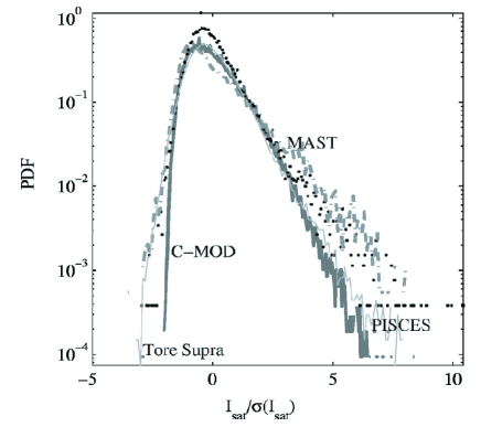
Figure 1: The PDF plot of the ion saturation current in the Tore Supra (solid line), Alcator C-Mod (thick solid line), MAST (dashed-dotted line), and PISCES (dots). The ion saturation current was normalized to the standard deviation and the integral of the four PDFs is set equal to 1. Figure reprinted with permission from Ref. Antar et al. (2003) (http://link.aip.org/link/?PHPAEN/10/419/1), Fig. 3, Copyright 2003, American Institute of Physics.

Bursty dynamics is characterized by strongly non-Gaussian PDFs and non-vanishing probabilities of extreme events. In such dynamical systems, the higher order moments are commonly used to determine the scaling properties of the fluctuating fields. The non–Gaussian features are usually quantified in terms of skewness and kurtosis of the PDF of fluctuating fields. For a centered random variable $\tilde{x}$, i.e. $\left<\tilde{x}\right>$=0, with variance $\sigma^{2}$, skewness is defined by the $S\equiv\left<\tilde{x}^{3}\right>/\sigma^{3}$ and the kurtosis (in the newer literature) by $K\equiv\left<\tilde{x}^{4}\right>/\sigma^{4}-3$. Skewness is a measure of asymmetry of a PDF; if the left tail is more pronounced than the right tail, the PDF has negative skewness and when the reverse is true, it has positive skewness. Kurtosis measures the excess probability (flatness) in the tails, where excess is defined in relation to a Gaussian distribution. For Gaussian distributions both $S$ and $K$ are equal to zero.

Using ten thousand observed density fluctuation signals measured in TORPEX, Labit et al. Labit et al. (2007) showed that a unique parabolic scaling relation holds, $K=1.502S^{2}-0.226$, between the skewness $S$ and the kurtosis $K$ (see Figure 1 of Reference Labit et al. (2007)). It was also shown that the PDFs of the measured signals, including those characterized by a negative skewness can be described by a special case of the Beta distribution. The density fluctuations were associated with regimes of drift–interchange (D-I) turbulence generated in regions of bad magnetic field curvature and convected away by the $E\times B$ fluid motion.

Remarkably, there is a striking similarity of the observed $K$–$S$ scaling with that of sea surface temperature (SST) fluctuations that are governed by advection through ocean currents Sura and Sardeshmukh (2008). Sura and Sardeshmukh Sura and Sardeshmukh (2008) proposed a nonlinear Langevin model that can predict the observed scaling in some limits of the model parameters while Krommes Krommes (2008) generalized it to include linear waves - an essential feature of D-I turbulence - and he numerically calculated the associated PDF that includes four indepedent parameters. The fact that the same scaling applies to different physical situations leads to conjecturing that the scaling arises due to basic constraints. The general mathematical constraints on the $K-S$ relation, as arise from the definition of kurtosis and skewness Sattin et al. (2009), do not provide any insight about the observed scaling. A recent comprehensive study on the observed $K-S$ scaling between various fusion devices showed that the data align along parabolic curves Sattin et al. (2009). A phenomenological model using the assumption that the fluctuating signals include a linear combination of two basis (Gamma or Beta ditributions) PDFs attempting to accommodate experimental evidence was also provided. However, the large number of the free parameters entering to the model and the small difference between using one or a sum of two Beta PDFs make the model less flexible Sattin et al. (2009).

It becomes evident that these observations among different physical systems reveal a universal character associated with strongly non–Gaussian processes. However, the key question is what kind of underlying mechanism is responsible for the universally observed statistical features and what PDF can describe them. In this Letter, a univariate model for the statistical description of bursty fluctuations is presented, using as an example the aforementioned plasma edge density fluctuations. Furthermore, the associated PDF is derived and it is shown that it recovers the universally observed distributions, documented in Ref. Antar et al. (2003) and the remarkable parabolic scaling between skewness and kurtosis as well, documented in Ref. Labit et al. (2007). The derived results have universal character, and thus may be applicable to all aforementioned physical systems.

The non–linear processes described by the standard models of turbulence in magnetized plasma are quadratic and are linked with small or large scale convection processes attributed to electric drifts. Thus, it is natural one to assume that the universally observed statistical characteristics associated with the bursty behavior of fluctuations may be attributed to processes that emerge from the non-linear quadratic interaction between turbulent fields. However, extreme statistical features are expected to appear when strong non–Gaussian processes coexist with Gaussian ones. In order to describe the associated universal statistical properties, we propose a univariate non-Gaussian process $W(t)$ given by:

$$W(t)=\frac{Z(t)-\left<Z(t)\right>}{\sigma_{0}}+\gamma\frac{Z^{2}(t)-\left<Z^{2}(t)\right>}{\sigma_{0}^{2}}$$ (1)

which results from the superposition of a Gaussian $Z(t)$ (with standard deviation $\sigma_{0}$) with a non-Gaussian process attributed to the square of $Z(t)$. The latter corresponds to the strongest quadratic non-linearity that may arise due to the interaction of fluctuating fields. The coefficient $\gamma$, in front of the quadratic non–Gaussian component is a parameter that measures the deviation of $W(t)$ from Gaussianity. The process $W(t)$ may well describe extreme bursty behavior of fluctuations that is characterized by non-linear structures (blobs, avaloids) that travel (convect) through a sea of Gaussian fluctuations. Figure 2 presents some typical time series $W(t)$ calculated from Eq. (1) by using a centered random Gaussian fluctuation $Z(t)$. In all cases the bursty nature of $W(t)$ is evident. For the sake of simplicity, from now on, we drop the dependence of $Z$ and $W$ on time and consider that $Z$ is a centered Gaussian process. It should be noted here that the process described by Eq. (1) has been presented in the literature Lenschow et al (1994) as a characteristic simple-to-construct non-Gaussian process and was used as an example for the calculation of the systematic errors of covariances and moments up to fourth order of non-Gaussian time series.

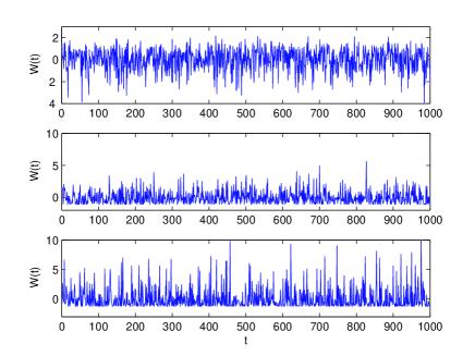
Figure 2: (a) Example of bursty time–series $W(t)$ for different values of $\gamma$: (a) -0.11, (b) 0.031, (c) 0.98, corresponding to negative (top), positive (middle), and significantly large positive (bottom) skewed distributions respectively.

For the derivation of the PDF $p(w)$ of the random process $W(t)$, we express the cumulative distribution function (CDF) $P(w)$ as follows

$$P(w)=\Pr\left({W\leq w}\right)=\Pr\left({\gamma\left({Z-z_{1}}\right)\left({Z-z_{2}}\right)\leq 0}\right)$$ (2)

where $z_{1}$ and $z_{2}$ are the roots of the polynomial

$$f(Z)=\gamma\frac{Z^{2}-{\sigma_{0}}^{2}}{{\sigma_{0}}^{2}}+\frac{Z}{\sigma_{0}}-w.$$ (3)

Equation 2 can be expressed in terms of the CDF $P(Z)$ at $z=z_{1},~{}z_{2}$ and $p(w)$ can be derived by a simple differentiation that leads to the following expression:

$$p\left(w\right)=\left\{{\begin{array}[]{*{20}c}{0,{\rm{\;\;\;when\;\;\;}}\lambda_{w}\equiv 4\gamma(w-w_{0})<0\mbox{ else; }}\\ {\sqrt{\frac{{2}}{{\pi}{\lambda_{w}}}}{\cosh\left(\frac{\sqrt{\lambda_{w}}}{4\gamma^{2}}\right)}\exp\left({-\frac{1+\lambda_{w}}{8\gamma^{2}}}\right),}\end{array}}\right.$$ (4)

where $w_{0}=-(4\gamma)^{-1}-\gamma$. The value and the sign of parameter $\gamma$ controls the shape and the range of non-zero values of $p(w)$. For $\gamma=0$, the $p(w)$ reduces to that of a centered Gaussian random process. For $\gamma>0$ ($\gamma<0$) a cut off value $w_{0}$ exists and $p(w)$ gets asymmetric presenting long tails in the positive (negative) axis (cf. Figure 3). The minimum (in absolute sense) value of the cut-off is equal to $w_{0m}=\pm 1$ and corresponds to $\gamma=\mp 1/2$. Note, that the same analytic expression for $p(w)$ can also be derived by noticing that the non-Gaussian process $W$ can be re-written in terms of a scaled and shifted non-central chi-squared random process with one degree of freedom,

$$W=w_{0}+\gamma\left({\frac{Z}{{\sigma_{0}}}+\frac{1}{{2\gamma}}}\right)^{2}$$ (5)

and using the expression of non-central chi-squared PDF along with standard transform techniques of random variables.

In Fig. 4, we have plotted $p(w)$ choosing positive values of $\gamma$ that range up to $\gamma=0.2$. The resulting distributions exhibit the same behavior with the measured distributions of plasma edge density fluctuations, as have been observed in several magnetic confinement devices and presented here in Fig. 1. Note, that the characteristic clustering of the PDF curves around $0.05$ for values around $2.5$ which is experimentally observed (cf. Fig. 1) is recovered by the distribution $p(w)$ (cf. Figs. 3 and 4) - independently on the value of $\gamma>0$ - a characteristic that is not recovered in the plots of PDF in Ref. Krommes (2008). Similar features appear also in the PDF of the x–ray observations associated with anomalous transport in accretion disks (cf. Fig. 8 of Ref. Geobel et al. (2002)).

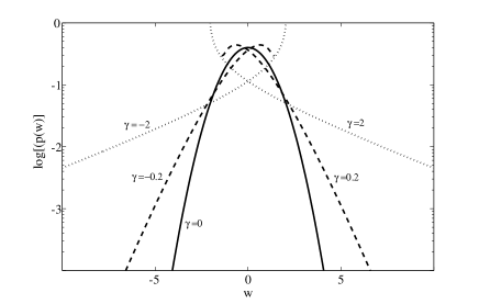
Figure 3: The family of distributions $p(w)$, for different values of $\gamma=-2,~{}-0.02,~{}0,~{}0.02\mbox{ and }2$. The symmetry with respect to $\gamma$ is evident. As $\gamma$ increases the absolute value of the cut–off decreases (increases) for $\gamma<0.5$ ($\gamma>0.5$).

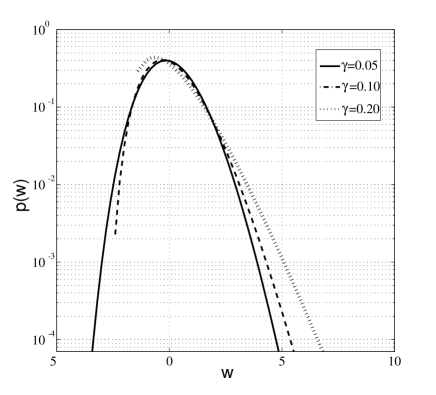
Figure 4: The family of distributions $p(w)$, for $\gamma=0.05,~{}0.1\mbox{ and }0.2$. The resulting PDFs recover the universally observed distributions presented at Fig. 1.

Unlike, to the BHP distribution [13] which does not have any free parameter, $p(w)$ depends on $\gamma$ such that its higher order moments can receive multiple values. Furthermore, the existence of a single free parameters allows $p(w)$ to be used for the fitting of experimentally observed distributions. The high order moments of multivariate Gaussian processes can be determined by a simple method based on the Wicks theorem. All odd moments are zero and all even moments can be reduced to homogeneous polynomials. For the considered process $W$, the values of skewness and kurtosis depend on the value of $\gamma$ and are given by Lenschow et al (1994),

$$S=2\gamma\frac{3+4\gamma^{2}}{(1+2\gamma^{2})^{3/2}}\mbox{ and }K=48\gamma^{4}\frac{1+\gamma^{2}}{(1+2\gamma^{2})^{2}}$$ (6)

For $\gamma=0$, the process $W$ is Gaussian and $K=S=0$. As $\left|\gamma\right|$ increases kurtosis and skewness converge to their extreme values $K_{max}=12$ and $S_{max}=\pm 2^{3/2}$, respectively. Noticeably, these values agree with the range of the values reported in the Letter by Garcia et al Garcia et al (2004), in which the authors investigate intermittent transport in plasma edge using extensive numerical simulations that take into account the presence of SOL.

Using the parabolic ansatz, $K=aS^{2}+b$ for the parametric relations in Eq. (6), it can be easily found that

$$a(\gamma)=12\frac{(1+\gamma^{2})(1+2\gamma^{2})}{(3+4\gamma^{2})^{2}},$$ (7)

and $b=0$. The function $a(\gamma)$ converges rapidly to the value $a=3/2$, which is exactly the value of the universally observed parabolic scaling, reported in Refs. Labit et al. (2007); Krommes (2008); Sura and Sardeshmukh (2008).

It is interesting to compare the derived $K-S$ curve of Eq. (6), to that attributed to a quadratic product of two central Gaussian processes $Z_{1},~{}Z_{2}$, i.e. $W_{\Gamma}=\gamma_{\Gamma}Z_{1}Z_{2}$. Here $\gamma_{\Gamma}$ denotes the correlation between the Gaussian fields. For $Z_{1}=Z_{2}$ and $\gamma_{\Gamma}=1$, the PDF of $W_{\Gamma}$ is simply the chi-squared distribution with one degree of freedom. The associated PDF $p(W_{\Gamma})$ has been presented in Ref. Carreras et al. (1996), and the corresponding values of skewness and kurtosis were found equal to:

$$S_{\Gamma}=-2\gamma_{\Gamma}\frac{3+\gamma_{\Gamma}^{2}}{(1+\gamma_{\Gamma}^{2})^{3/2}}\mbox{ and }K_{\Gamma}=6\frac{1+6\gamma_{\Gamma}^{2}+\gamma_{\Gamma}^{4}}{(1+\gamma_{\Gamma}^{2})^{2}},$$ (8)

respectively. The parabolic relation, $K=a_{\Gamma}S^{2}+b_{\Gamma}$, between $S_{\Gamma}$ and $K_{\Gamma}$, results to the derivation of the following coefficients:

$$a_{\Gamma}=\frac{6(1+\gamma_{\Gamma}^{2})}{(3+\gamma_{\Gamma}^{2})^{2}}\mbox{ and }b_{\Gamma}=6.$$ (9)

Note that for $\left|\gamma_{\Gamma}\right|=1$, the values of kurtosis and skewness are equal to $K_{max}$ and $S_{max}$, while for $\gamma_{\Gamma}=0$, are equal to $6$ and $0$, respectively.

Equations (6) and (9) define a closed curve in the $K-S$ space for continuous values of the parameters $\gamma$ and $\gamma_{\Gamma}$ respectively (see Fig. 5). The low boundary of the curve corresponds to extreme bursty processes $W$ given by Eq. (1) and distributed according to $p(w)$, while the upper boundary corresponds to $W_{\Gamma}$ which is distributed according to the “local flux PDF” (see Eq. (7) in Ref. Carreras et al. (1996)). The clustering of the $K-S$ values around the $K=1.5S^{2}$ curve is patently seen in Fig. 1 of Reference Labit et al. (2007) and in Fig. 3 of Reference Sura and Sardeshmukh (2008).

It is straightforward to show numerically, that for non–Gaussian processes (described by second order polynomials of Gaussians) the “cloud” of $K-S$ points fall into (not shown here) the closed curve. The latter follow a parabolic trend – similar to the experiments Sattin et al. (2009) – with scaling that depends on the selection of the polynomial coefficients. Furthermore, for processes described by higher order Gaussian polynomials the “cloud” follows also parabolic trend including much higher values of $K$ and $S$.

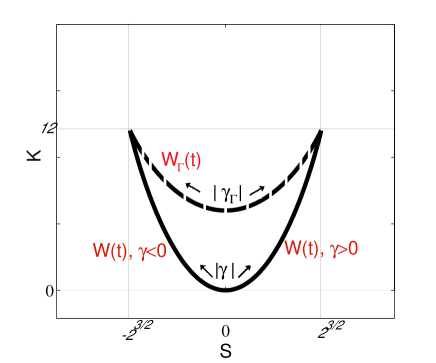
Figure 5: The $K-S$ curve for stochastic processes described by quadratic polynomial of gaussians. The solid line corresponds to $W(t)$ and the dashed line to $w_{\Gamma}(t)$ process.

In conclusion, a univariate stochastic model for the description of extreme bursty fluctuations $W$ based on generic properties of quadratic non-linearities is presented. The model and the associated probability distribution function describe statistical properties of the SOL density fluctuations which are governed by the $E\times B$ convection. The universal character of the stochastic process stems from the fact that the associated extreme PDF recovers properties of variabilities (density/sea temperature/x-ray intensity) observed at boundary regions (SOL/sea surface/accretion edge) of different physical processes that are characterized by convection (electric drift/ocean current/rotation). The proposed univariate stochastic model describes the statistical characteristics of these relaxation phenomena at a state of extreme statistical behavior. It is evident that the parabolic relation between $S$ and $K$ when observed provide relevant information about the underlying processes.

IS acknowledges fruitful discussions with Yu. Khotyaintsev, F. Lepreti and A. Anastasiadis. DCN acknowledges support from the Oak Ridge National Laboratory, managed by UT-Battelle, LLC, for the U.S. This work was supported under the Contract of Association ERB 5005 CT 99 0100 between the European Atomic Energy Community and the Hellenic Republic. The content of the publication is the sole responsibility of its author(s) and it does not necessarily represent the views of the Commission or its services.

References

- Benkadda et al. (1994) S. Benkadda, et al., Phys. Rev. Lett. 73, 3403 (1994).
- Jha et al. (1992) R. Jha, P.K. Kaw, and S.K. Mattoo, Phys. Rev. Lett. 69, 1375 (1992).
- Antar et al (2001) G.Y. Antar, S.I. Krasheninnikov, and P. Devynck, Phys. Rev. Lett. 87, 065001 (2001).
- Antar et al. (2003) G.Y. Antar, et al., Phys. Plasmas 10, 419 (2003).
- Dendy and Chapman (2006) R.O. Dendy, and S.C. Chapman, Plasma Phys. Control. Fusion 48, B313 (2006).
- Geobel et al. (2002) D. Geobel, et al., Astron. Astroph. 385, 693 (2002).
- Labit et al. (2007) B. Labit, et al., Phys. Rev. Lett. 98, 255002 (2007).
- Krommes (2008) J.A. Krommes, Phys. Plasmas 15, 030703 (2008).
- Sura and Sardeshmukh (2008) P. Sura, and P.D. Sardeshmukh, J. Phys. Oceanogr. 38, 639 (2008).
- Sattin et al. (2009) F. Sattin, et al., Phys. Scr. 79, 045006 (2009).
- Sattin et al. (2009) F. Sattin, et al., Plasma Phys. Control. Fusion 51, 055013 (2009).
- Lenschow et al (1994) D.H. Lenschow, J. Mann, L. Kristensen, Jour. Atm. Ocean. Techn. 11, 661 (1994).
- Bramwell et al (1998) S.T. Bramwell, P.C.W. Holdsworth, J.-F Pinton, Nature 396, 552 (1998).
- Garcia et al (2004) O.E. Garcia, et al., Phys. Rev. Lett. 92, 165003 (2004).
- Carreras et al. (1996) B.A. Carreras, C. Hidalgo, E. Sanchez, Phys. Plasmas 3, 2664 (1996).