Non-Nearest-Neighbor Interactions in Nonlinear Dynamical Lattices

Abstract

We revisit the theme of non-nearest-neighbor interactions in nonlinear dynamical lattices, in the prototypical setting of the discrete nonlinear Schrödinger equation. Our approach offers a systematic way of analyzing the existence and stability of solutions of the system near the so-called anti-continuum limit of zero coupling. This affords us a number of analytical insights such as the fact that, for instance, next-nearest-neighbor interactions allow for solutions with nontrivial phase structure in infinite one-dimensional lattices; in the case of purely nearest-neighbor interactions, such phase structure is disallowed. On the other hand, such non-nearest-neighbor interactions can critically affect the stability of unstable structures, such as topological charge $S=2$ discrete vortices. These analytical predictions are corroborated by numerical bifurcation and stability computations.

I Introduction

Undoubtedly, the discrete nonlinear Schrödinger (DNLS) equation is one of the most fundamental nonlinear lattice dynamical models. Part of its relevance is due to its being one of the main discrete analogs of the famous (and integrable in 1+1 dimensions) continuum nonlinear Schrödinger (NLS) equation sulem ; trub . The latter is encountered in a wide spectrum of applications; it is the relevant dispersive envelope wave model for the electric field in optical fibers hasegawa ; malomed , for the self-focusing and collapse of Langmuir waves in plasma physics zakh1 ; zakh2 or for the description of freak waves (the so-called rogue waves) in the ocean onofrio .

On the other hand, the DNLS model is of physical interest in its own right within a diverse host of applications; see the reviews IJMPB ; joh_rev , as well as the recent book kev_book . One of the principal directions that spurred a considerable interest in the DNLS model was the area of the nonlinear optics of fabricated AlGaAs waveguide arrays 7 . In this seting, a plethora of important phenomena have been experimentally investigated including discrete diffraction, Peierls barriers (the energetic barrier that a wave needs to overcome to move over a lattice), diffraction management (the periodic alternation of the diffraction coefficient) 7a and gap solitons (structures localized due to nonlinearity in the gap of the underlying linear spectrum) 7b among others eis3 . More recently, quasi-periodic recent1 and even completely disordered recent2 variants of such waveguide lattices have been constructed, allowing the observation of localization type phenomena (even within the linear regime for ones of the Anderson type). Many of these results and the corresponding theoretical activity that they triggered has been summarized in a number of reviews see e.g. review_opt ; general_review .

Another independent and considerably different physical setting where DNLS-type models naturally arise is that of Bose-Einstein condensates (BECs) trapped within periodic (so-called, optical lattice) potentials created by counter-propagating laser beams in one-, two- or even three- spatial dimensions bloch . This area of atomic physics has also experienced a huge growth over the past few years, including the prediction and manifestation of modulational instabilities (i.e., the instability of spatially uniform states towards spatially modulated ones) pgk , the observation of gap solitons markus , Landau-Zener tunneling (tunneling between different bands of the periodic potential) arimondo and Bloch oscillations (for matter waves subject to combined periodic and linear potentials) bpa_kasevich among many other salient features; reviews of the theoretical and experimental findings in this area have also recently appeared in konotop ; markus2 .

Our aim in the present communication is to consider a somewhat non-standard variant of the DNLS equation, namely one in which the interaction kernel within the linear term allows interactions among any set of neighbors. Such, so-called, nonlocal versions of the DNLS model have been abundantly considered in the past, yielding numerous interesting features. In particular, it was shown, for instance, that, if the interaction strength decays sufficiently slowly as a function of distance, it can give rise to bistability of fundamental solitary waves (centered on a single site) nonlocalBistability , which may find applications in their controllable switching switchingBistable . Dynamical lattices with long-range interactions also serve as models for energy and charge transport in biological molecules EnergyChargeTransportBiomolecules . Systems including the next-nearest-neighbor (NNN) interaction have also been proposed as models of polymers nextnearestPolymer , as well as in the case of optical waveguide arrays near the zero-dispersion point borisus . Nonlinear lattice models with competing short- and long-range interactions were studied not only in one, but also in two dimensions 2DcompetingShortLongRange . Lastly, it is relevant to mention that quantum DNLS models with nonlocal interactions were another subject of study (by means of the Bethe ansatz) quantum . It should be pointed out that such longer-range interactions are often directly relevant to physical applications. For example, in the case of the waveguide arrays, the NNN interaction is also, in principle, present yet its relative strength depends on the ratio of the separation between adjacent cores to the wavelength of light. A specific, zigzag-shaped, model of an optical array involving a NNN coupling was introduced in Ref. Cyprus , allowing for essentially arbitrary ratios of nearest- to next-nearest-neighbor interactions, depending on the specific geometry. Lately, long-range interactions, especially of a dipolar type have become of considerable interest in BECs due to the significant component of dipole-dipole interactions in ⁵²Cr. These effects, as well as the significant component of studies of such dipolar BECs in optical lattices have recently been summarized in pfau .

The scope of the present communication is to explore the non-local variant of DNLS in the vicinity of the so-called anti-continuum (AC) limit, where all individual sites (i.e., waveguides in optics or wells of the optical lattice in BEC) are uncoupled. From there, in the spirit of peli1d , we can develop a perturbative expansion using the strength of the interactions as the relevant small parameter. This allows us to derive conditions for the persistence of states near the AC-limit, as well as to formulate a framework to address their linear stability. Both the existence conditions, as well as the stability conditions allow us to infer valuable conclusions. The existence conditions suggest (and numerical computations corroborate) the possibility that solutions with a nontrivial phase distribution may arise in the 1d setting, a feature which is absent in the case of nearest-neighbor (NN) interactions; even the sole inclusion of NNN interactions allows to achieve this feature. On the other hand, concerning stability, the inclusion of NNN interactions may also play an important role, as we illustrate with a two-dimensional example: the stabilization of a topological charge $S=2$ vortex (which is unstable in the presence of NN interactions) is numerically observed and analytically justified.

Our analytical considerations are presented in section II, while section III is devoted to the corresponding numerical results (and their comparison to theory). Finally, section IV summarizes our findings and suggests a number of interesting future directions.

II Analytical Considerations

Our nonlocal variant of the DNLS equation will be of the following form:

$$i\dot{u}_{n}-u_{n}+|u_{n}|^{2}u_{n}=-\varepsilon\sum_{m=1}^{N}k_{nm}u_{m}$$ (1)

where the overdot denotes temporal (in the case of BECs in optical lattices) or spatial (in the case of waveguide arrays) derivatives, $n$ denotes the site index (waveguide index in the optical case, or optical lattice well in BECs), and $\epsilon$ controls the strength of the coupling among sites, which is also determined by the “coupling matrix” with elements $k_{nm}$. The dependent variable $u$ represents the complex envelope of the electric field in optics, or the complex wavefunction of the BEC in atomic physics. The AC limit is defined by $\varepsilon=0$, in which case the unperturbed energy of the uncoupled oscillators reads

$$E_{0}(u)=\sum_{n}|u_{n}|^{2}-\frac{1}{2}|u_{n}|^{4}.$$ (2)

Once the inter-site coupling is turned on, the relevant perturbation in the energy reads:

$$E_{1}(u)=-\epsilon\sum_{n,m=1}^{N}k_{nm}\left(u_{n}^{\star}u_{m}+u_{n}u_{m}^{\star}\right)$$ (3)

Notice that at the AC limit, the solutions for the excited oscillators will be $u_{n}=e^{i\theta_{n}}$, where the $\theta_{n}$’s are arbitrary phase parameters ($u_{n}=0$ corresponds to the non-excited sites).

To determine the persistence of the waves, as was illustrated in todd_pers (see also the general framework of bjorn or the nearest-neighbor case of peli1d ) one has to evaluate the perturbed energy at the unperturbed limit solution, in which case, we can straightforwardly evaluate it to be:

$$E_{1}=-\sum_{n,m=1}^{N}2k_{nm}\cos(\theta_{n}-\theta_{m}),$$ (4)

where $N$ is the number of excited (adjacent in this case, for simplicity, –although the theory can be appropriately generalized for non-adjacent) oscillators. The general persistence conditions then read $\partial_{\theta_{n}}E_{1}=0$ todd_pers ; bjorn , i.e., the unperturbed wave needs to correspond to an extremum of the perturbation energy in order to persist. This leads to the condition

$$\sum_{m\neq n}k_{nm}\sin(\theta_{n}-\theta_{m})=0.$$ (5)

On the other hand, the general stability theory of bjorn (again see peli1d for a particular application in the case of nearest-neighbor interactions) allows us to quantify the bifurcation of the $N-1$ eigenvalues from $\lambda=0$. There are $N$ eigenvalues at $\lambda=0$ when $\varepsilon=0$, and only one of them remains there for finite $\varepsilon$, due to the U$(1)$ symmetry and associated phase invariance, while $N-1$ acquire small (O$(\sqrt{\varepsilon})$ or smaller) values, as the sites become coupled. These eigenvalues satisfy the reduced eigenvalue problem bjorn

$$(D_{0}\lambda^{2}+M)v=0,$$ (6)

where

$$D_{0} = -I_{N}$$ (7)

$$M_{nm} = \partial_{\theta_{n}\theta_{m}}^{2}E_{1},$$ (8)

i.e., the stability is effectively determined by the Jacobian of the persistence conditions. It is worthwhile to note that this general formulation encompasses the nearest-neighbor one of peli1d as a special case.

The above formulas, namely Eq. (5) describing the existence and Eqs. (6)-(8) quantifying the stability under weak coupling are the main analytical results of the present study, which we now proceed to utilize in specific applications where additional (to the nearest neighbor) interactions exist.

III Numerical Results

In this section, we apply the above analysis to a few select cases where interactions other than purely nearest neighbor ones are included, so as to provide a sense of the kind of additional features that such settings may entail and how these features are brought forth through the above analysis. We start with what arguably can be dubbed the simplest extension of NN interactions, namely the inclusion of the NNN ones which is directly physically realizable, as per the setting of Cyprus .

We start from the case of equal NN and NNN interactions only, i.e., $k_{nm}=\delta_{m,n\pm 1}+\delta_{m,n\pm 2}$, where $\delta$ denotes the Kronecker $\delta$. Considering then a $N=3$ site configuration (the smallest one that “perceives” of the presence of the NNN interaction), it is straightforward to intuitively realize that this is essentially the analog of an equilateral triangle where all pairwise interactions exist and are equal to each other. This is a situation that has been considered both in DNLS kody_pre (see also the early work of chris_e ) and in Klein-Gordon vass1 ; vass2 type settings, motivated by applications of triangular lattices in photorefractive crystals and dusty plasmas. It has been illustrated therein that the fundamental linearly stable 3-excited-site configuration is that of a so-called vortex of topological charge $S=1$, namely a situation where the phase runs from $0$ at the first excited site, to $2\pi/3$ at the second one and $4\pi/3$ at the third one. Remarkably, all configurations with the standard (from the NN setting of peli1d ) case of $0$ or $\pi$ phases, are unstable. Equally importantly the NN case, as per the arguments of peli1d , never allows for the existence of phases other than $0$ or $\pi$ in 1d configurations. Hence, one of the principal features of these non-nearest-neighbor interactions is that they may enable configurations that would not be possible in standard NN settings. Moreover, as indicated above in this case, the eigenvalues can be analytically computed (through a discrete Fourier transform applied to the “triangle” of sites (which has periodic boundary conditions). This can be found to lead to the eigenvalues

$$\lambda_{j}=\pm\sqrt{8\varepsilon\cos(\Delta\theta)\sin^{2}\left(\frac{\pi j}{3}\right)}$$ (9)

for $j=1,2,3$. The stable case features the relative phase between adjacent sites $\Delta\theta=2\pi/3$ and yields a double pair of imaginary eigenvalues $\pm\sqrt{3\varepsilon}i$ which are compared to the full numerical results in Fig. 1 (also the analytical existence prediction for the relative angle among adjacent sites is tested through the numerical results of the figure). Good agreement is obtained between the analytical and numerical results in both existence and stability, for small values of $\varepsilon$, while, as expected, relevant deviations increase for larger values of the perturbation parameter. We also note in passing that the non-trivial phase vortex structure becomes unstable eventually in an oscillatory way due to a complex quartet of eigenvalues for $\varepsilon>0.116$ as also illustrated in Fig. 1, due to the collision of one of the imaginary pairs with the continuous spectrum extending above $\lambda=i$ (and below $\lambda=-i$).

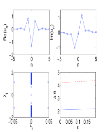
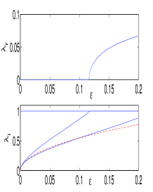
Figure 1: The figure shows a 3-site solution with a nontrivial phase distribution $(0,2\pi/3,4\pi/3)$ in the 1d case with equal nearest and next-nearest-neighbor interaction strengths of unity, i.e., $k_{n,n\pm 2}=k_{n,n\pm 1}=1$. The first two panels in the top row show the real and imaginary part of the solution for $\varepsilon=0.15$, while the bottom left shows the corresponding spectral plane $(\lambda_{r},\lambda_{i})$ of the linearization eigenvalues $\lambda=\lambda_{r}+i\lambda_{i}$. The second panel of the bottom row shows the relative phases $\Delta\theta=\theta_{2}-\theta_{1}$ (blue solid line) and $\theta_{3}-\theta_{1}$ (red dashed line), which does not change significantly from its anti-continuum limit as $\varepsilon$ is increased. Lastly, the top right and bottom rightmost panels show the maximal real eigenvalue (larger than zero -and hence giving rise to an instability- for $\varepsilon>0.116$) and lowest imaginary eigenvalues, respectively (blue solid lines). The theoretical prediction for the latter is given by the red dashed line.

To illustrate the generality of our analytical considerations in settings other than the special, degenerate case of Fig. 1, we considered another physically realizable (as per Cyprus ) case where $k_{n,n\pm 2}=0.7k_{n,n\pm 1}=0.7$ (while all other interactions are absent). Again, focusing on the 3-site interaction, we realize that the three persistence conditions can be explicitly solved, yielding two possible scenarios. Either $\sin(\theta_{n}-\theta_{m})=0$ for all combinations of $n,m\in\{1,2,3\}$ or $\theta_{1}-\theta_{2}=\theta_{2}-\theta_{3}$ and $\cos(\theta_{1}-\theta_{2})=-k_{n,n+1}/(2k_{n,n+2})$. Notice that this encompasses the discussion of equal strengths of NN and NNN interactions as a special case and additionally reveals the condition under which the nontrivial phase distributions discussed above can generally materialize, since it is necessary that $|k_{n,n+1}/(2k_{n,n+2})|<1$. In the case of Fig. 2, the analytical prediction yields a phase difference of $\theta_{1}-\theta_{2}=2.3664$ ($\theta_{1}-\theta_{3}$ is twice that) in excellent agreement with the numerical observations. Notice also that the relative phases appear to depend only weakly on $\varepsilon$ in the continuations over the latter parameter shown in Fig. 2. Additionally, our stability considerations allow us in this case to obtain the analytical predictions for the two (now split due to the asymmetry in the interactions) pairs of small eigenvalues $\lambda=\pm\sqrt{4.2858\varepsilon}i$ and $\lambda=\pm\sqrt{1.3714\varepsilon}i$. Good agreement is once again found with the full numerical linear stability results for small couplings $\varepsilon$, while this agreement deteriorates when increasing the coupling. The solution becomes unstable once again through the oscillatory instability arising upon collision (for $\varepsilon>0.109$) of the larger one among the above 2 pairs with the continuous spectrum.

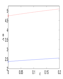
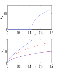
Figure 2: An example of weaker (than nearest-neighbor) next-nearest-neighbor interaction strength with $k_{n,n\pm 2}=0.7$ while $k_{n,n\pm 1}=1$: the phase distribution is shown on the left (and its anti-continuum limit, as theoretically predicted is depicted by squares), while the predictions of the linear stability analysis (red dashed lines) are compared with the full numerical results (blue solid lines) as a function of $\varepsilon$ on the right. The real part of the corresponding eigenvalues becomes nonzero for $\varepsilon>0.109$ (as shown in the top right panel).

However, the above features such as the nontrivial phase distribution are not a unique feature of cases with just NN and NNN interactions. As an alternative example that shares these features, we consider the case where $k_{nm}=\delta_{m,n\pm 1}+\delta_{m,n\pm 2}+\delta_{m,n\pm 3}$. Contrary to what might be naively expected, we do not find here the generalization of a vortex including 4-sites. While the lowest order persistence conditions are satisfied by such a solution, higher order ones are not. However, this does not preclude the existence of genuinely complex solutions with a complicated phase structure. An example of this kind involving $7$ sites is shown in Fig. 3. The phases of the 7 excited sites are found at the AC limit to be $\theta_{1}=0$ (since one of them can always be chosen arbitrarily), $\theta_{2}=3.2831$, $\theta_{3}=1.8780$, $\theta_{4}=4.0894$, $\theta_{5}=0.01766$ and $\theta_{7}=1.8957$. Then, the corresponding eigenvalue predictions from the reduced eigenvalue problem are: $\lambda=\pm\sqrt{7.0792\varepsilon}i$, $\lambda=\pm\sqrt{6.875\varepsilon}i$, $\lambda=\pm\sqrt{4.2006\varepsilon}i$, $\lambda=\pm\sqrt{3.4994\varepsilon}i$, $\lambda=\pm\sqrt{0.2248\varepsilon}i$, $\lambda=\pm\sqrt{0.1334\varepsilon}i$. These are compared to the full numerical eigenvalues of the problem (as are the existence results) in Fig. 3. Despite the complexity of the eigenvalue structure, the quality of the agreement between theory and numerics is clear from the eigenvalue inset and the phase comparisons (near the AC limit). Notice that the solution becomes unstable for $\varepsilon>0.062$ due to collision of the largest of the above pairs with the continuous spectrum and increasingly so due to additional collisions for $\varepsilon>0.088$, $\varepsilon>0.121$ and $\varepsilon>0.128$.

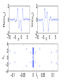
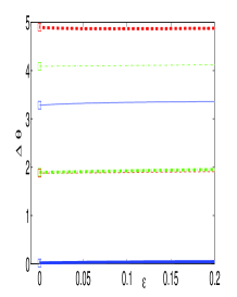
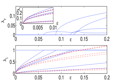
Figure 3: A more complicated 1d example of a 7-site wave with nontrivial phase distribution for $k_{n,n\pm 1}=k_{n,n\pm 2}=k_{n,n\pm 3}=1$. The top left panels show the real and imaginary parts of the solution and its spectral plane for $\varepsilon=0.2$; the top right shows the relative phases $\Delta\theta_{i}=\theta_{i}-\theta_{1}$ for $i=2,\dots,7$ ($i=2$: blue solid, $i=3$: red dashed, $i=4$: green dash-dotted, $i=5$ thick blue solid, $i=6$: thick red dashed, $i=7$: thick green dash-dotted); the theoretical anti-continuum limit is given by squares. Lastly, the bottom panels show the six relevant eigenvalues (blue solid lines) and the corresponding theoretical predictions (red dashed lines). The real (top) and imaginary (bottom) parts of the eigenvalues are given – it is clear that the solution becomes unstable for $\varepsilon>0.062$. This inset contains a blowup of the imaginary parts for small $\varepsilon$ to showcase the agreement between numerics and theory.

As our last example and in order to demonstrate a case where the non-nearest-neighbor interactions have a direct impact on stability, we consider a prototypical two-dimensional case of an unstable structure with vorticity, namely the vortex of topological charge $S=2$. It is well-known peli1d ; old that this structure is unstable and a considerable effort has been invested in stabilizing it either via defects pgk_djf or geometrically through a rhombic configuration joh2 . Here, we illustrate that NNN interactions can also play a stabilizing role for this coherent structure. In particular, we examined a special case (but verified that the result was also robust for other choices), where $k_{{\bf n},{\bf m}}=1$ for $|{\bf n}-{\bf m}|=1$, $k_{{\bf n},{\bf m}}=1$ for $|{\bf n}-{\bf m}|=2$, while $k_{{\bf n},{\bf m}}=2$ for $|{\bf n}-{\bf m}|=\sqrt{2}$ (where the last choice was made because of the two lattice paths connecting the relevant neighbors). In this case, (but also with other choices of the relative weights), it is straightforward to show that the square configuration with $\theta_{j}=j\pi/2$, where $j=1,\dots,8$ remains a solution and that the corresponding reduced eigenvalue problem has a single eigenvalue pair of $\lambda=\pm 4\sqrt{\varepsilon}i$, another single pair of $\lambda=\pm\sqrt{8\varepsilon}i$, and a quadruple pair of $\lambda=\pm 2\sqrt{\varepsilon}i$ (while one pair is exactly at 0 and one is 0 to leading order but also remains imaginary at higher orders). This stabilized variant of the $S=2$ vortex can be observed in Fig. 4, where again the analytical predictions are compared to the numerical results, yielding increasingly good agreement once again for smaller values of $\varepsilon$. Notice that the solution becomes destabilized for $\varepsilon>0.032$, while additional quartets arise for $\varepsilon>0.048$, $\varepsilon>0.074$ and $\varepsilon>0.087$.

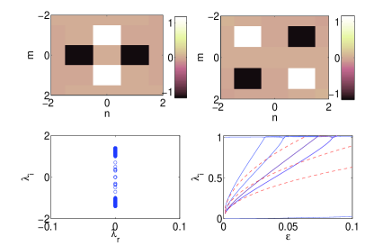
Figure 4: An example of the stabilized $S=2$ vortex for $\varepsilon=0.02$ (the real contour of the solutions is shown in the top left and the imaginary one in the top right). The spectral plane indicating the stability of the solution is shown in the bottom left while the corresponding numerically obtained (imaginary) eigenvalues are in the bottom right (blue solid, as compared with the red dashed theoretical prediction). The solution becomes unstable for $\varepsilon>0.032$.

IV Conclusions

In the present work, we have revisited the theme of non-nearest-neighbor interactions in settings of the discrete nonlinear Schrödinger type motivated by applications especially in optical (but also in other areas such as atomic) physics. We illustrated that an analytical approach enables a number of interesting conclusions and possibilities that did not seem to have been realized before, to the best of our knowledge, both as concerns the existence problem on the infinite lattice, and as concerns the stability properties in the context of localized solitary wave solutions.

In particular, we focused on the vicinity of the anti-continuum limit of vanishing coupling. There, we could obtain explicit conditions for the persistence of localized modes, as well as analytical predictions for the eigenvalues of linearization around such solutions. This analysis allows to conclude that the non-nearest-neighbor setting has a number of special properties. More specifically, even just next-nearest-neighbor interactions (but also more general ones) create the possibility for solutions with more complicated phase profiles than just phases of $0$ and $\pi$ as was the case for nearest-neighbor interactions peli1d . On the other hand, these longer range interactions can play a critical role in the stability of solutions that were found to be unstable in the nearest-neighbor setting. We presented a particular such example in the case of the topological charge $S=2$ discrete two-dimensional vortex.

Although our work lays the ground for understanding some of the main features of these non-nearest-neighbor settings, a number of interesting questions are still outstanding. In particular, it would be interesting if something could be said more generally about the type of solutions (and phase distributions) afforded by interactions of different range/decay properties. On the other hand, it would be interesting if a general classification of stability could also be made for different types of intereaction kernels, in higher or even in one dimension. These questions are presently under investigation and will be reported in future publications.

The warm hospitality of the Kirchoff Institute for Physics and of the Institute for Physics of the University of Heidelberg (at the last stage of this work), as well as the support of NSF-DMS-0349023, NSF-DMS-0806762 and of the Alexander von Humboldt Foundation are gratefully acknowledged.

References

- (1) C. Sulem and P.L. Sulem, The Nonlinear Schrödinger Equation, Springer-Verlag (New York, 1999).
- (2) M.J. Ablowitz, B. Prinari and A.D. Trubatch, Discrete and Continuous Nonlinear Schrödinger Systems, Cambridge University Press (Cambridge, 2004).
- (3) A. Hasegawa, Solitons in Optical Communications, Clarendon Press (Oxford, NY 1995).
- (4) B.A. Malomed, Progr. Opt. 43, 71 (2002).
- (5) V.E. Zakharov, Collapse and Self-focusing of Langmuir Waves, Handbook of Plasma Physics, (M.N. Rosenbluth and R.Z. Sagdeev eds.), vol. 2 (A.A. Galeev and R.N. Sudan eds.), 81-121, Elsevier (1984).
- (6) V.E. Zakharov, Sov. Phys. JETP 35, 908 (1972).
- (7) M. Onorato, A.R. Osborne, M. Serio, and S. Bertone Phys. Rev. Lett. 86, 5831 (2001)
- (8) P.G. Kevrekidis, K.Ø. Rasmussen and A.R. Bishop, Int. J. Mod. Phys. B 15, 2833 (2001).
- (9) J. C. Eilbeck and M. Johansson, in Localization and Energy Transfer in Nonlinear Systems, edited by L. Vázquez, R. S. MacKay, and M. P. Zorzano (World Scientific, Singapore, 2003), p. 44.
- (10) P.G. Kevrekidis, The Discrete Nonlinear Schrödinger Equation, Springer-Verlag (Heidelberg, 2009).
- (11) H.S. Eisenberg, Y. Silberberg, R. Morandotti, A.R. Boyd and J.S. Aitchison, Phys. Rev. Lett. 81, 3383 (1998).
- (12) R. Morandotti, U. Peschel, J.S. Aitchison, H.S. Eisenberg and Y. Silberberg, Phys. Rev. Lett. 83, 2726 (1999); H.S. Eisenberg, Y. Silberberg, R. Morandotti and J.S. Aitchison, Phys. Rev. Lett. 85, 1863 (2000).
- (13) D. Mandelik, R. Morandotti, J.S. Aitchison, and Y. Silberberg Phys. Rev. Lett. 92, 93904 (2004).
- (14) R. Morandotti, H.S. Eisenberg, and Y. Silberberg, M. Sorel and J. S. Aitchison, Phys. Rev. Lett. 86, 3296 (1999).
- (15) Y. Lahini, R. Pugatch, F. Pozzi, M. Sorel, R. Morandotti, N. Davidson and Y. Silberberg, Phys. Rev. Lett. 103, 013901 (2009).
- (16) Y. Lahini, A. Avidan, F. Pozzi, M. Sorel, R. Morandotti, D.N. Christodoulides and Y. Silberberg, Phys. Rev. Lett. 100, 013906 (2008).
- (17) D. N. Christodoulides, F. Lederer, and Y. Silberberg, Nature 424, 817 (2003); A. A. Sukhorukov, Y. S. Kivshar, H. S. Eisenberg, and Y. Silberberg, IEEE J. Quant. Elect. 39, 31 (2003).
- (18) S. Aubry, Physica 103D, 201 (1997); S. Flach and C. R. Willis, Phys. Rep. 295, 181 (1998); D. K. Campbell, S. Flach, and Y. S. Kivshar, Phys. Today, January 2004, p. 43; S. Flach and A.V. Gorbach, Phys. Rep. 467, 1 (2008).
- (19) S. Burger, F. S. Cataliotti, C. Fort, P. Maddaloni, F. Minardi and M. Inguscio, Europhys. Lett. 57, 1 (2002).
- (20) A. Smerzi, A. Trombettoni, P. G. Kevrekidis, and A. R. Bishop, Phys. Rev. Lett. 89, 170402 (2002); F.S. Cataliotti, L. Fallani, F. Ferlaino, C. Fort, P. Maddaloni and M. Inguscio, New J. Phys. 5, 71 (2003).
- (21) B. Eiermann, Th. Anker, M. Albiez, M. Taglieber, P. Treutlein, K.-P. Marzlin, and M.K. Oberthaler Phys. Rev. Lett. 92, 230401 (2004)
- (22) M. Jona-Lasinio, O. Morsch, M. Cristiani, N. Malossi, J. H. Müller, E. Courtade, M. Anderlini, and E. Arimondo Phys. Rev. Lett. 91, 230406 (2003)
- (23) B.P. Anderson and M.A. Kasevich, Science 282, 1686 (1998).
- (24) V. A. Brazhnyi and V. V. Konotop, Mod. Phys. Lett. B 18, 627 (2004); P. G. Kevrekidis and D. J. Frantzeskakis, Mod. Phys. Lett. B 18, 173 (2004).
- (25) O. Morsch and M. Oberthaler, Rev. Mod. Phys. 78, 179 (2006).
- (26) Y.B. Gaididei, S.F. Mingaleev, P.L. Christiansen, and K.Ø. Rasmussen, Phys. Rev. E 55, 6141 (1997); K.O. Rasmussen, P.L. Christiansen, M. Johansson, Y.B. Gaididei, and S.F. Mingaleev, Physica D 113, 134 (1998).
- (27) M. Johansson, Y.B. Gaididei, P.L. Christiansen, and K.Ø. Rasmussen, Phys. Rev. E 57, 2739 (1998).
- (28) S.F. Mingaleev, P.L. Christiansen, Y.B. Gaididei, M. Johansson, and K.O. Rasmussen, J. Biol. Phys. 25, 41 (1999).
- (29) D. Hennig, Europ. Phys. J. B 20, 419 (2001).
- (30) P.G. Kevrekidis, B.A. Malomed, A. Saxena, A.R. Bishop and D.J. Frantzeskakis, Physica D 183, 87 (2003).
- (31) P.G. Kevrekidis, Y.B. Gaididei, A.R. Bishop, and A. Saxena, Phys. Rev. E 64, 066606 (2001).
- (32) A.G. Choudhury and A.R. Chowdhury, Physica Scripta 53, 129 (1996).
- (33) D.N. Christodoulides and N. Efremidis, Phys. Rev. E 65, 056607 (2002).
- (34) T. Lahaye, C. Menotti, L. Santos, M. Lewenstein and T. Pfau, arXiv:0905.0386.
- (35) D.E. Pelinovsky, P.G. Kevrekidis and D.J. Frantzeskakis, Physica D 212, 1 (2005); D.E. Pelinovsky, P.G. Kevrekidis and D.J. Frantzeskakis, Physica D 212, 20 (2005); M. Lukas, D. Pelinovsky and P.G. Kevrekidis, Physica D 237, 339 (2008).
- (36) T. Kapitula, Physica D 156, 186 (2001).
- (37) T. Kapitula, P.G. Kevrekidis, and B. Sandstede, Physica D 195, 263 (2004).
- (38) K.J.H. Law, P.G. Kevrekidis, V. Koukouloyannis, I. Kourakis, D.J. Frantzeskakis, and A.R. Bishop, Phys. Rev. E 78, 066610 (2008).
- (39) J.C. Eilbeck, P.S. Lomdahl and A.C. Scott, Physica D 16, 318 (1985). We should note that this pioneering work considered a few configurations also studied herein such as the equal NN and NNN case, as well as that of equal NN, NNN and third neighbor interactions, but did so purely in the 3- and 4-site chain respectively, without considering the generalization to the infinite lattice.
- (40) V. Koukouloyannis, and R.S. MacKay, J. Phys. A: Math. Gen. 38, 1021 (2005).
- (41) V. Koukouloyannis, P.G. Kevrekidis, K.J.H. Law, I. Kourakis and D.J. Frantzeskakis, arXiv:0906.2726.
- (42) B.A. Malomed and P.G. Kevrekidis, Phys. Rev. E 64, 026601 (2001).
- (43) P.G. Kevrekidis and D.J. Frantzeskakis, Phys. Rev. E 72, 016606 (2005).
- (44) M. Öster and M. Johansson, Phys. Rev. E 73, 0666608 (2006).