Analytical Study of Adversarial Strategies in Cluster-based Overlays

Abstract

Scheideler has shown that peer-to-peer overlays networks can only survive Byzantine attacks if malicious nodes are not able to predict what is going to be the topology of the network for a given sequence of join and leave operations. In this paper we investigate adversarial strategies by following specific games. Our analysis demonstrates first that an adversary can very quickly subvert DHT-based overlays by simply never triggering leave operations. We then show that when all nodes (honest and malicious ones) are imposed on a limited lifetime, the system eventually reaches a stationary regime where the ratio of polluted clusters is bounded, independently from the initial amount of corruption in the system.

1 Introduction

The adoption of peer-to-peer overlay networks as a building block for architecting Internet scale systems has raised the attention of making these overlays resilient not only to benign crashes, but also to more malicious failure models for the peers [5, 12, 13, 14]. As a result, Byzantine-resilient overlay systems have been proposed (e.g., [6, 4, 1]). The key to achieve Byzantine resilience in a peer-to-peer overlay is to prevent malicious peers from isolating correct ones. This in turn, can only be achieved if malicious peers are not able to predict what will be the topology of the overlay for a given sequence of join and leave operations. Hence, a prerequisite for this condition to hold is to guarantee that malicious nodes are well-mixed with honest ones, that is nodes identifiers randomness is continuously preserved. Unfortunately, targeted join/leave attacks may quickly endanger the relevance of such assumption. Actually by holding a logarithmic number of IP addresses, an adversary can very easily and efficiently disconnect some target from the rest of the system. This can be achieved in a linear number of offline trials [2]. Awerbuch and Scheideler [3] have analysed several ways to make overlay networks provably robust against different forms of malicious attacks, and in particular targeted join/leave attacks, through competitive algorithms. All these solutions are based on the introduction of locally induced churn to prevent the adversary from thwarting randomness. The same authors have shown that despite the high level of randomness introduced in each of these strategies, most of them are either incorrect, or they involve tight synchronization among nodes which becomes unbearable in the context we address, namely targeted and frequent join/leave attacks. The other proposed approach based on globally induced churn, enforce limited lifetime for each node in the system. However, these solutions keep the system in an unnecessary hyper-activity, and thus need to impose strict restrictions on nodes joining rate which clearly limit their applicability to open systems.

In this paper we propose to leverage the power of clustering to design a practically usable solution that preserves randomness under an $\epsilon$-bounded adversary. Our solution relies on the clusterized version of peer-to-peer overlays combined with a mechanism that allows the enforcement of limited nodes lifetime. Clusterized versions of structured-based overlays are such that clusters of nodes substitute nodes at the vertices of the graph. Cluster-based overlays have revealed to be well adapted for efficiently reducing the impact of churn on the system and/ or in greatly reducing the damage caused by failures—assuming that failures assumptions hold anywhere and at any time in the system [1, 9, 6].

The contributions of the paper are two-fold. First we investigate adversarial strategies by following specific games. Our analysis demonstrates that an adversary can very quickly subvert cluster-based overlays by simply never triggering leave operations. We then show that when nodes are imposed on a limited lifetime and under the assumption that we are able to enforce the adversary to leave the system after expiration of its ID, the system eventually reaches a stationary regime where the ratio of polluted clusters is bounded. Second we propose a simple and generic mechanism to limit nodes lifetime in those systems.

The remainder of this paper is as follows: In Section 2 we briefly describe the main features of cluster-based overlays, and propose a mechanism that enables the enforcement of limited nodes lifetime. In Section 3, we model adversarial behaviours through the use of games. We study the outcome of these games by using a Markovian analysis. In this section, we consider a non restricted adversary. Section 4 is devoted to the same study in the case of a restricted adversary. Finally, we conclude with future works.

2 Cluster-based DHT Overlays in a Nutshell

In this section we first present the common features of cluster-based overlays and then present different join/leave strategies whose long term behaviors are analysed in Section 3.

Clusterized versions of structured-based overlays are such that clusters of nodes substitute nodes at the vertices of the graph. Nodes are uniquely identified with some $m$-bit string randomly chosen from an ID-space. Identifiers (IDs) are derived by using standard collision-resistant one-way hash functions (e.g., [10]). Each graph vertex is composed of a set of nodes self-organised within a cluster according to some distance metrics (e.g., logical or geographical). Clusters in the system are uniquely labelled. Size of each cluster is lower (resp. upper) bounded. The lower bound, named $S_{min}$ in the following, usually satisfies some constraint based on the assumed failure model. For instance $S_{min}\geq 4$ allows Byzantine tolerant agreement protocols to be run among these $S_{min}$ nodes [8]. The upper bound, that we call $S_{max}$, is typically in $\mathcal{O}(logN)$, where $N$ is the current number of nodes in the system, to meet scalability requirements. When a cluster size reaches these bounds, cluster-based overlays react by respectively splitting that cluster into two smallest clusters or by merging it with its closest cluster neighbours. Finally for most of the cluster-based overlays, operations (join, leave, merge, and split) are poly-logarithmic in the number of nodes in the system.

In the present work we assume that at cluster level nodes are organised as core and spare members. Members of the core set are primarily responsible for handling messages routing and clusters operations. Management of the core set is such that its size is maintained to constant $S_{min}$. Spare members are the complement number of nodes in the cluster. In contrast to core members, they are not involved in any of the overlay operations. Rationale of this classification is two-fold: first it allows to introduce the unpredictability required to deal with Byzantine attacks through a randomized core set generation algorithm. Second it limits the management overhead caused by the natural churn present in typical overlay networks through the spare set management.

Specifically we consider the following join and leave operations:

• join(p): when a peer joins a cluster, it joins it as a spare member.

• leave(p): When a peer $p$ leaves a cluster either $p$ belongs to the spare set or to the core set. In the former case, core members simply update their spare view to reflect $p$’s departure, while in the latter case, the core view maintenance procedure is triggered. Two different maintenance policies are implemented. The first one, referred in the following as policy 1, simply consists in replacing the left core member by one randomly chosen spare member. The second one, referred as policy 2, consists in refreshing the whole core set by choosing $S_{min}$ random peers within the cluster.

For space reasons we do not give any detail regarding the localization of a cluster nor its creation/split/merge process. None of these operations are necessary for the understanding of our work. The interested reader is invited to read their description in the original papers (e.g. [1, 9, 6]).

2.1 Implementing a limited nodes lifetime

To implement limited nodes lifetime, we propose to proceed as follows: Peers identifiers are generated based on certificates acquired at trustworthy Certification Authorities (CAs). Identifiers (denoted IDs) are generated as the result of applying a hash function to some of the fields of a X.509 [7] certificate. To enforce all peers, including malicious ones, leaving and rejoining the system from time to time, we add a incarnation number to the fields that appear in the peer’s certificate that will be hashed to generate the peer’s ID. The incarnation number limits the lifetime of IDs. The current incarnation $k$ of any peer is given by the following expression $k=\lceil(CT-IVT)\rceil/IL$, where $IVT$ is the initial validity time of the peer’s certificate, $CT$ is the current time, and $IL$ is the length of the lifetime of each peer’s incarnation. Thus, the $k^{th}$ incarnation of a peer $p$ expires when its local clock reads $IVT+k*IL$. At this time $p$ must rejoin the system using its $(k+1)^{th}$ incarnation. The $IVT$ is one of the fields in the peer’s certificate and since certificates are signed by the CA, it cannot be unnoticeably modified by a malicious peer. Moreover, a certificate commonly contains the public key of the certified entity. This way, messages exchanged by the peers can be signed using this key, preventing malicious peers from unnoticeably altering messages originated from other peers in the system. Messages must contain the certificate of their issuer, so as to allow recipients to validate them. Therefore, at any time, any peer can check the validity of the ID of any other peers in the system, by simply calculating the current incarnation of the other peer and generating the corresponding ID. If some peer detects that the ID of one of its neighbours is not valid then it cuts its connection with it. Note that because clocks are loosely synchronised, it is possible that a correct peer is still using its ID for incarnation $k$ when other correct peers would expect it to be in incarnation $k+1$. To mitigate this problem, we assume that any correct peer may have two subsequent valid incarnation numbers, for a fixed grace window $GW$ of time that encompasses the expiration time of an incarnation number ($GW$ is the maximum deviation of the clocks of any two correct peers). More precisely, at any time $t$, both incarnation $k$ and $k^{\prime}$ are valid, where: $k=\lceil(t-GW/2-IVT)\rceil/IL$, and $k^{\prime}=\lceil(t+GW/2-IVT)\rceil/IL$. Notice that this means that although at any time $t$ each peer $p$ has a single incarnation number that it uses to define its current ID, other peers calculate two possible incarnation numbers for $p$. These are frequently equal, but may differ when $p$’s local time is close to the expiration time of its current/last incarnation.

3 Modelling the adversarial strategy as a game

In this section, we investigate the previously described policies (policy 1 and 2). We model adversarial behavior by focusing on specific games. Both games intend to prevent the adversary from elaborating deterministic strategies to win. These games are played in the following context. There is a potentially infinite number of balls in a bag, with a proportion $\mu$ of red balls and a proportion $1-\mu$ of white balls, $\mu$ being a constant in $(0,1)$. White (resp. red) balls are indistinguishable. Red balls are owned by the adversary. In addition to the bag, there are two urns, named $\mathcal{C}$ and $\mathcal{S}$. Initially, $c+s$ balls are drawn from the bag such that $c$ of them are thrown into urn $\mathcal{C}$, and the other $s$ ones are thrown into urn $\mathcal{S}$. We denote by $C_{r}$ (resp. $S_{r}$) the number of red balls in $\mathcal{C}$ (resp. $\mathcal{S}$). It is easily checked that $C_{r}$ and $S_{r}$ are independent and have a binomial distribution, i.e. for $x=0,\ldots,c$ and $y=0,\ldots,s$, we have

$$\begin{array}[]{rcl}\mathbbm{P}\{C_{r}=x,S_{r}=y\}&=&\mathbbm{P}\{C_{r}=x\}\mathbbm{P}\{S_{r}=y\}\\ &=&{c\choose x}\mu^{x}(1-\mu)^{c-x}{s\choose y}\mu^{y}(1-\mu)^{s-y}.\end{array}$$ (1)

This joint distribution represents the initial distribution of the process detailed below. Each game is a succession of rounds $r_{1},r_{2},\ldots$ during which the game rule described in Figure 1 is applied. Rules are oblivious to the colour of the balls, that is, they cannot distinguish between the white and the red balls.

  /* First game */ /* stage 1 */ draw ball $b_{0}$ from $\mathcal{C}\cup\mathcal{S}$ /* stage 2 */ if $b_{0}$ was in $\mathcal{S}$ then throw $b_{0}$ into the bag draw ball $b_{2}$ from the bag throw it into $\mathcal{S}$ else throw $b_{0}$ into the bag draw ball $b_{1}$ from $\mathcal{S}$ throw it into $\mathcal{C}$ draw ball $b_{2}$ from the bag throw it into $\mathcal{S}$                        /* Second game */ /* stage 1 */ draw ball $b_{0}$ from $\mathcal{C}\cup\mathcal{S}$ /* stage 2 */ if $b_{0}$ was in $\mathcal{S}$ then throw $b_{0}$ into the bag draw ball $b_{2}$ from the bag throw it into $\mathcal{S}$ else throw $b_{0}$ into the bag draw $c$ balls from $\mathcal{S}\cup\mathcal{C}$ throw these $c$ balls into $\mathcal{C}$ draw one ball $b_{2}$ from the bag throw it in $\mathcal{S}$  

Figure 1: Rule of the first and second game.

The goal of the adversary is to get a quorum $Q$ of red balls in both urns $\mathcal{C}$ and $\mathcal{S}$ so that the number of red balls in $\mathcal{C}$ is bound to continuously exceed $\lfloor(c-1)/3\rfloor$. An intuition of why having more than $\lfloor(c-1)/3\rfloor$ red balls in urn $\mathcal{C}$ is necessary for polluting it is related to agreement problems in distributed systems in presence of Byzantine processes. The value of quorum $Q$ is derived in the sequel. The adversary may at any time inspect both urns and bag to elaborate adversarial strategies to win the game. In particular it may not follow the rule of the games by preventing its red balls from being extracted from both urns. Specifically, at stage 1 of both games, if the drawn ball $b_{0}$ is red then the adversary puts back the ball into the urn from which it has been drawn. Stage 2 is not applied, and a new round is triggered. Clearly this strategy ensures that the number of red balls in $\mathcal{C}\cup\mathcal{S}$ is monotonically non decreasing.

We model the effects of these rounds using a homogeneous Markov chain denoted by $X=\{X_{n},n\geq 0\}$ representing the evolution of the number of red balls in both urns $\mathcal{C}$ and $\mathcal{S}$. More formally, the state space $S$ of $X$ is defined by $S=\{(x,y)\mid 0\leq x\leq c,\;0\leq y\leq s\},$ and, for $n\geq 1$, the event $X_{n}=(x,y)$ means that, after the $n$-th transition or $n$-th round, the number of red balls in urn $\mathcal{C}$ is equal to $x$ and the number of red balls in urn $\mathcal{S}$ is equal to $y$. The transition probability matrix $P$ of $X$ depends on the rule of the given game and on the adversarial behaviours. This matrix is detailed in each of the following subsections. In all the cases, the initial state $X_{0}$ is given by $X_{0}=(C_{r},S_{r})$ and its probability distribution is denoted by the row vector $\alpha$ which is given by relation (1), i.e. $\alpha(x,y)=\mathbbm{P}\{X_{0}=(x,y)\}=\mathbbm{P}\{C_{r}=x,S_{r}=y\}.$

We define a state as polluted if in that state urn $\mathcal{C}$ contains more than $\lfloor(c-1)/3\rfloor$ balls. In the following, we denote by $c^{\prime}$ the value $\lfloor(c-1)/3\rfloor$. Conversely, a state that is not polluted is said safe. The subset of safe states, denoted by $A$, is defined as: $A=\{(x,y)\mid 0\leq x\leq c^{\prime},\;0\leq y\leq s\},$ while the set of polluted states, denoted by $B$, is the subset $S-A$, i.e. $B=\{(x,y)\mid c^{\prime}+1\leq x\leq c,\;0\leq y\leq s\}.$ We partition matrix $P$ in a manner conformant to the decomposition of $S=A\cup B$, by writing

$$P=\left(\begin{array}[]{cc}P_{A}&P_{AB}\\ P_{BA}&P_{B}\\ \end{array}\right),$$

where $P_{A}$ (resp. $P_{B}$) is the sub-matrix of dimension $|A|\times|A|$ (resp. $|B|\times|B|$), containing the transitions between states of $A$ (resp. $B$). In the same way, $P_{AB}$ (resp. $P_{BA}$) is the sub-matrix of dimension $|A|\times|B|$ (resp. $|B|\times|A|$), containing the transitions from states of $A$ (resp. $B$) to states of $B$ (resp. $A$). We also partition the initial probability distribution $\alpha$ according to the decomposition $S=A\cup B$, by writing $\alpha=(\alpha_{A}\;\;\alpha_{B}),$ where sub-vector $\alpha_{A}$ (resp. $\alpha_{B}$) contains the initial probabilities of states of $A$ (resp. $B$).

3.1 First game

Regarding the first game, computation of the probabilities of the transition matrix is illustrated in Figure 2. In this tree, each edge is labelled by a probability and its corresponding event following the rule of the game (see Figure 1). This figure can be interpreted as follows: At round $r$, $r\geq 1$, starting from state $(x;y)$ (root of the tree) the Markov chain can transit to four different states, namely $(x;y)$, $(x;y+1)$, $(x+1;y)$, and $(x+1;y+1)$ (leaves of the tree). The probability associated to each one of these transitions is obtained by summing the products of the probabilities discovered along each path starting from the root to the leaf corresponding to the target state.

Figure 2: Transition diagram for the computation of the transition probability matrix $P$ for the first game.

We can easily derive the transition probability matrix $P$ of the Markov chain $X$ chain associated to this game. For all $x\in\{0,\ldots,c\}$ and for all $y\in\{0,\ldots,s\}$, we have

$$p_{(x,y),(x,y)} = \left(\frac{c}{c+s}\right)\left(\frac{x}{c}+\left(\frac{c-x}{c}\right)\left(\frac{s-y}{s}\right)(1-\mu)\right)+\left(\frac{s}{s+c}\right)\left(\frac{y}{s}\mu+1-\mu\right)$$

$$p_{(x,y),(x,y+1)} = \left(\left(\frac{c}{c+s}\right)\left(\frac{c-x}{c}\right)+\left(\frac{s}{s+c}\right)\right)\left(\frac{s-y}{s}\right)\mu\;\;\;\mbox{ for }y\leq s-1$$

$$p_{(x,y),(x+1,y-1)} = \left(\frac{c}{c+s}\right)\left(\frac{c-x}{c}\right)\frac{y}{s}(1-\mu)\;\;\;\mbox{ for }x\leq c-1\mbox{ and }y\geq 1$$

$$p_{(x,y),(x+1,y)} = \left(\frac{c}{c+s}\right)\left(\frac{c-x}{c}\right)\frac{y}{s}\mu\;\;\;\mbox{ for }x\leq c-1.$$

In all other cases, transition probabilities are null.

Clearly, the adversary wins the game when the process $X$ reaches the subset of states $B$ from which it cannot exit. Thus quorum $Q=\{(x,y)\mid(x,y)\in B\}.$ with $B$ the set of polluted states. By the rule of the game, one can never escape from these states to switch to safe states since the number of red balls in $\mathcal{C}$ is non decreasing. Thus there is a finite random time $T$ after which the process $X$ is absorbed within $B$. Thus we have $P_{BA}=0$. The Markov chain $X$ is reducible and the states of $A$ are transient, which means that matrix $I-P_{A}$ is invertible, where $I$ is the identity matrix of the right dimension which is $|A|$ here. Specifically $T$, the time needed to reach subset $B$, is defined as $T=\inf\{n\geq 0\mid X_{n}\in B\}.$ The cumulative distribution function of $T$ is easily derived as

$$\mathbbm{P}\{T\leq k\}=1-\alpha_{A}(P_{A})^{k}\mathbbm{1},$$ (2)

where $\mathbbm{1}$ is the column vector of the right dimension with all components equal to $1$. The expectation of $T$ is given by

$$E(T)=\alpha_{A}(I-P_{A})^{-1}\mathbbm{1},$$ (3)

3.2 Second game

By proceeding similarly as above, we can derive the following transitions of process $X$ associated to the second game. Briefly, when the game starts in state $(x,y)$ at round $r$, it remains in state $(x,y)$ during the round if either ball $b_{0}$ is red or $b_{0}$ is white, and has been drawn from $\mathcal{S}$, and $b_{2}$ is white. It changes to state $(x,y+1)$ if $b_{0}$ is white, it has been drawn from $\mathcal{S}$, and $b_{2}$ is red. Finally the game switches to state $(k,x+y-k+\ell)$, where $k$ is an integer $k=0,\ldots,c^{\prime}$ and $\ell=0$ or $1$ if $b_{0}$ is white, it has been drawn from $\mathcal{C}$, and the renewal process leads to the choice of $k$ red balls. For all $x\in\{0,\ldots,c\}$ and $y\in\{0,\ldots,s\}$, we have

$$p_{(x,y),(x,y)} = \left(\frac{c}{c+s}\right)\left(\frac{x}{c}\mu q(x,x+y-1)+\frac{c-x}{c}(1-\mu)q(x,x+y)\right)+$$

$$\left(\frac{s}{c+s}\right)\left(\frac{s-y}{s}\left(1-\mu\right)+\frac{y}{s}\mu\right)$$

$$p_{(x,y),(x,y+1)} = \left(\frac{c}{c+s}\right)\frac{x}{c}\mu q(x,x+y)+\left(\frac{s}{c+s}\right)\left(\frac{s-x}{c}\mu\right)\mbox{ for }y\leq s-1$$

$$p_{(x,y),(x,y-1)} = \left(\frac{c}{c+s}\right)\frac{x}{c}(1-\mu)q(x,x+y-1)+\left(\frac{s}{c+s}\right)\left(\frac{s-x}{c}\mu\right)\mbox{ for }y\geq 1$$

$$p_{(x,y),(k,x+y-k)} = \left(\frac{c}{c+s}\right)\left(\frac{c-x}{c}\right)\left(1-\mu\right)q(k,x+y)$$

$$\mbox{ for }\max(0,x+y-s)\leq k\leq\min(c,x+y)\mbox{ and }k\neq x$$

$$p_{(x,y),(k,x+y-k+1)} = \left(\frac{c}{c+s}\right)\left(\frac{c-x}{c}\right)\mu q(k,x+y)$$

$$\mbox{ for }\max(0,x+y+1-s)\leq k\leq\min(c,x+y+1)\mbox{ and }k\neq x$$

where

$$q(x,x+y)=\frac{{\displaystyle{x+y\choose x}{c+s-1-(x+y)\choose c-x}}}{{\displaystyle{c+s-1\choose c}}}$$

is the probability of getting $x$ red balls when $c$ balls are drawn, without replacement, in an urn containing $x+y$ red balls and $c+s-1-(x+y)$ white balls, referred to as the hypergeometric distribution. In all other cases, transition probabilities are null.

In contrast to the first game, this game alternates between safe and polluted states. After a random number of these alternations the process ends by entering a set of closed polluted states. Indeed, by the rule of the game, one can escape finitely often from polluted state $(x;y)$ to switch back to a safe state as long as $(x;y)$ satisfies $c^{\prime}+1\leq x+y\leq s+c^{\prime}$ (there are still sufficiently many white balls in both $\mathcal{C}$ and $\mathcal{S}$ so as to successfully withdrawing $c$ balls such that $\mathcal{C}$ can be reverted to a safe state). However, there is a time $T_{D}$ when state $(x;y)$, with $x+y\geq s+c^{\prime}+1$, is entered. From $T_{D}$ onwards, going back to safe states is impossible. Thus at time $T_{D}$ the adversary wins the game. Hence an interesting metrics to be evaluated is the total time spent by the process in safe states before being definitely absorbed in polluted states.

Formally, we need to decompose the set $B$ of polluted states into two subsets $C$ and $D$ defined by $C=\{(x;y)\mid c^{\prime}+1\leq x+y\leq s+c^{\prime},\;c^{\prime}+1\leq x\leq c,\;0\leq y\leq s\},$ and $D=\{(x;y)\mid x+y\geq s+c^{\prime}+1,\;0\leq y\leq s\}.$ Subsets $A$ and $C$ are transient and subset $D$ is a closed subset. We partition matrix $P$ and initial probability vector $\alpha$ following the decomposition of $S=A\cup C\cup D$, by writing

$$P=\left(\begin{array}[]{ccc}P_{A}&P_{AC}&0\\ P_{CA}&P_{C}&P_{CD}\\ 0&0&P_{D}\\ \end{array}\right)\ \mbox{and}\ \alpha=(\alpha_{A}\;\;\alpha_{C}\;\;\alpha_{D}).$$

Figure 3 illustrates the states partition of the process $X$.

Figure 3: An aggregated view of the Markov chain associated to the second game. Safe states are represented by A, and polluted states by C and D.

We are interested in the random variable $T_{A}$ which counts the total time spent in subset $A$ before reaching subset $D$. Following the result obtained in [11], we have, for every $k\geq 0$,

$$\mathbbm{P}\{T_{A}\leq k\}=1-vG^{k}\mathbbm{1},$$ (4)

where $v=\alpha_{A}+\alpha_{C}(I-P_{C})^{-1}P_{CA}\mbox{ and }G=P_{A}+P_{AC}(I-P_{C})^{-1}P_{CA}.$ The expected total time spent in $A$ is given by

$$E(T_{A})=v(I-G)^{-1}\mathbbm{1}.$$ (5)

Figure 4 compares the expectation of the time spent in safe states for both games. In accordance with the intuition, increasing the size of the urns augments the expected time spent in safe states of both games, i.e., $E(T)$ and $E(T_{A})$, independently of the ratio of red balls in the bag. Similarly, for a given cluster size, increasing the ratio of red balls in the bag drastically decreases both $E(T)$ and $E(T_{A})$. However surprisingly enough, increasing the level of randomness (game 2 vs. game 1) does not increase the resilience to the adversary behavior since the first game always overpasses the second one in expectation. It is even more true when $\mathcal{S}$ size is large with respect to $\mathcal{C}$ one. The intuition behind this fact is as follows: when $\mathcal{S}$ size is equal to 1, both games are equivalent as illustrated in Figure 4 for $s=1$. Now, consider the case where the size of $\mathcal{S}$ is large with respect to $\mathcal{C}$ one. First of all, note that the probability to draw a ball from $\mathcal{S}$ tends to $1$, and because the adversary never withdraw its red balls from any urns, the ratio of red balls within $\mathcal{S}$ is monotonically non decreasing. Hence, the ratio of red balls in $\mathcal{S}$ tends also to 1. With small probability, a ball from $\mathcal{C}$ is drawn. In the first game it is replaced with high probability by a red ball drawn from $\mathcal{S}$. Hence to reach a polluted state, at least $c^{\prime}$ white balls have to be replaced by red ones. While in the second game with high probability, the renewal of $\mathcal{C}$ reaches a polluted state in a single step. From this crude reasoning we can derive that the ratio of $E(T)$ over $E(T_{A})$ tends to $c^{\prime}$.

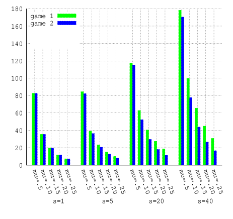
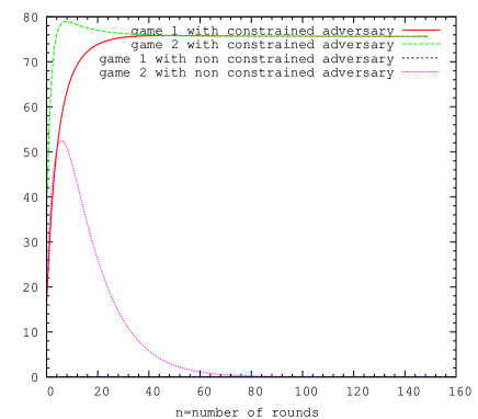
Figure 4: (a) Expectation of the number of rounds spent in safe states for games 1 and 2 function of $\mathcal{S}$ size and the ratio of malicious nodes $\mu$ as resp. given by relations (LABEL:eq:et) and (LABEL:eq:eta). (b) Mean number of safe clusters $E(N_{n})$ (relation (LABEL:eq:enn)) in function of the rounds number $n$ for both games and both kind of adversaries. There are l=100 clusters, and the ratio of red balls in the bag is equal to .25 and $c=7$. Note that the initial number of safe clusters is equal to 16.

4 Constraining the adversary

Our next step is to evaluate the benefit of constraining the adversary by limiting the sojourn time of its balls in both urns, so that randomness among red and white balls is continuously preserved. In the model we propose, we assume that the adversary cannot prevent red balls from being withdrawn for both urns.

By proceeding as in Sections 3.1 and 3.2, we can derive the transition probability matrix $P$ for both games. For all $x\in\{0,\ldots,c\}$ and $y\in\{0,\ldots,s\}$, the entries of $P$ are given, for the first game, by

$$p_{(x,y),(x,y)} = \frac{xy+(c(s-y)-xs)(1-\mu)}{(c+s)s})+\frac{y\mu+(s-y)(1-\mu)}{c+s}$$

$$p_{(x,y),(x,y-1)} = \frac{(x+s)y}{(c+s)s}(1-\mu)\mbox{ for }y\geq 1$$

$$p_{(x,y),(x,y+1)} = \left(\frac{c-x+s}{c+s}\right)\left(\frac{s-y}{s}\right)\mu\mbox{ for }y\leq s-1$$

$$p_{(x,y),(x+1,y-1)} = \frac{(c-x)y}{(c+s)s}(1-\mu)\mbox{ for }x\leq c-1\mbox{ and }y\geq 1$$ (6)

$$p_{(x,y),(x+1,y)} = \frac{(c-x)y}{(c+s)s}\mu\mbox{ for }x\leq c-1$$

$$p_{(x,y),(x-1,y)} = \frac{x(s-y)}{(c+s)s}(1-\mu)\mbox{ for }x\geq 1$$

$$p_{(x,y),(x-1,y+1)} = \frac{x(s-y)}{(c+s)s}\mu\mbox{ for }x\geq 1\mbox{ and }y\leq s-1.$$

In all other cases, transition probabilities are null. Similarly for second game , for all $x\in\{0,\ldots,c\}$ and $y\in\{0,\ldots,s\}$, we have

$$p_{(x,y),(x,y)} = \frac{xq(x,x+y-1)\mu+(c-x)q(x,x+y)(1-\mu)}{c+s}+\frac{y\mu+(s-y)(1-\mu)}{c+s}$$

$$p_{(x,y),(x,y-1)} = \frac{x}{c+s}q(x,x+y-1)(1-\mu)+\frac{y}{c+s}(1-\mu)\mbox{ for }y\geq 1$$

$$p_{(x,y),(x,y+1)} = \frac{c-x}{c+s}q(x,x+y)\mu+\frac{s-y}{c+s}\mu\mbox{ for }y\leq s-1$$

$$p_{(x,y),(k,x+y-k-1)} = \frac{x}{c+s}q(k,x+y-1)(1-\mu)$$

$$\mbox{ for }\max(0,x+y-1-s)\leq k\leq\min(c,x+y-1)\mbox{ and }k\neq x$$

$$p_{(x,y),(k,x+y-k)} = \frac{x}{c+s}q(k,x+y-1)\mu+\frac{c-x}{c+s}q{(k,x+y)}(1-\mu)$$

$$\mbox{ for }\max(0,x+y-s)\leq k\leq\min(c,x+y-1)\mbox{ and }k\neq x$$

$$p_{(x,y),(k,x+y-k+1)} = \frac{c-x}{c+s}q{(k,x+y)}\mu$$

$$\mbox{ for }\max(0,x+y+1-s)\leq k\leq\min(c,x+y)\mbox{ and }k\neq x,$$

where we set $q(u,v)=0$ when $u>v$. In all other cases, transition probabilities are null.

It is not difficult to see that none of the games exhibit an absorbing class of states (i.e., both games never ends). We have $P_{BA}\neq 0$ and the process $X$ is irreducible and aperiodic since at least one state has a transition to itself. The distribution of the time $T$ needed to reach subset $B$ is given, for every $k\geq 0$, by

$$\mathbbm{P}\{T\leq k\}=1-\alpha_{A}(P_{A})^{k}\mathbbm{1}.$$ (8)

We denote by $\pi$ the stationary distribution of the Markov chain $X$. The row vector $\pi$ is thus the solution to the linear system

$$\pi=\pi P\mbox{ and }\pi\mathbbm{1}=1.$$

As we did for row vector $\alpha$, we partition $\pi$ according to the decomposition $S=A\cup B$, by writing $\pi=(\pi_{A}\;\;\pi_{B}),$ where sub-vector $\pi_{A}$ (resp. $\pi_{B}$) contains the stationary probabilities of states of $A$ (resp. $B$).

Theorem 1

For both games 1 and 2, the stationary distribution $\pi$ is equal to $\alpha$, i.e. for all $x=0,\ldots,c$ and $y=0,\ldots,s$, we have

$$\lim_{n\longrightarrow\infty}\mathbbm{P}\{X_{n}=(x,y)\}=\alpha(x,y),$$

which is given by relation (1).

Proof. For space reasons, we omit the proof of the theorem. The interested reader is invited to read it in the Appendix.   

Theorem 1 is interesting in two aspects. First it shows that the stationary distribution $\pi$ is exactly the same for both games, and second, that this distribution is equal to the initial distribution $\alpha$. At a first glance, we could guess that this phenomenon is due to the fact that the Markov chain $X$ is the tensor product of two independent Markov chains, representing respectively the evolution of the red balls in $\mathcal{C}$ and $\mathcal{S}$. Although this is clearly not the case as the behavior of red balls in $\mathcal{C}$ depends on the behavior of red balls in $\mathcal{S}$. This holds for both games.

The stationary availability of the system defined by the long run probability to be in safe states is denoted by $P_{{\rm safe}}$ and is given by

$$P_{{\rm safe}}=\pi_{A}\mathbbm{1}=\sum_{x=0}^{c^{\prime}}{c\choose x}\mu^{x}(1-\mu)^{c-x}.$$

This probability can also be interpreted as the long run proportion of time spent in safe states. Note that the stationary distribution does not depend on the size of $\mathcal{S}$.

Now let us consider that we have $\ell$ identical and independent Markov chains $X^{(1)},\ldots,X^{(\ell)}$ on the same state space $S=A\cup\{S\setminus A\}$, with initial probability distribution $\beta$ and transition probability matrix $P$. The probability distribution $\beta$ represents the state $(0;0)$, i.e., the safest state. Each Markov chain models a particular cluster of nodes and, for $n\geq 0$, $N_{n}$ represents the number of safe clusters after the $n$-th round, i.e. the number of Markov chains being in subset $A$ after the $n$-th transition has been triggered, defined by

$$N_{n}=\sum_{j=1}^{\ell}1_{\{X_{n}^{(j)}\in A\}}.$$

The $\ell$ Markov chains being identical and independent, $N_{n}$ has a binomial distribution, that is, for $k=0,\ldots,\ell$, we have

$$\mathbbm{P}\{N_{n}=k\} = {\ell\choose k}\left(\mathbbm{P}\{X_{n}^{(1)}\in A\}\right)^{k}\left(1-\mathbbm{P}\{X_{n}^{(1)}\in A\}\right)^{\ell-k}$$

$$= {\ell\choose k}\left(\beta P^{n}\mathbbm{1}_{A}\right)^{k}\left(1-\beta P^{n}\mathbbm{1}_{A}\right)^{\ell-k}$$

and

$$E(N_{n})=\ell\beta P^{n}\mathbbm{1}_{A},$$

where $\mathbbm{1}_{A}$ is the column vector with the $i$-th entry equal to $1$ if $i\in A$ and equal to $0$ otherwise. If $N$ denotes the stationary number of safe clusters, we have, for $k=0,\ldots,\ell$,

$$\begin{array}[]{rcll}\mathbbm{P}\{N=k\}&=&{\ell\choose k}\left(\pi_{A}\mathbbm{1}\right)^{k}\left(1-\pi_{A}\mathbbm{1}\right)^{\ell-k}&\mbox{ for a constrained adversary }\\ &=&0&\mbox{ for a non constrained adversary}\end{array}$$

and

$$\begin{array}[]{rcll}E(N)&=&\ell\pi_{A}\mathbbm{1}&\mbox{ for a constrained adversary }\\ &=&0&\mbox{ for a non constrained adversary}\end{array}$$

These results are illustrated in Figure 4. We can observe that with a constrained adversary, the ratio of safe clusters tends to the same limit for both games, whatever the amount of initially safe clusters (less than a 1/4), while with a non constrained adversary eventually all the clusters get polluted.

5 Conclusion

In this paper, we have proposed a mechanism that enables the enforcement of limited nodes lifetime compliant with DHT-based overlays specificities. We have investigated several adversarial strategies. Our analysis has demonstrated that an adversary can easily subvert a cluster-based overlay by simply never triggering leave operations. We have then shown that when nodes have to regularly leave the system, eventually this one reaches a stationary regime where the ratio of malicious nodes is bounded.

For future work, we plan to implement this limited node lifetime mechanism in PeerCube to study its impact on the induced churn and its management overhead. We are convinced that this additional churn will be efficiently amortised thanks to the organisation of nodes in core and spare sets.

Appendix

• For both games 1 and 2, the stationary distribution $\pi$ is equal to $\alpha$, i.e. for all $x=0,\ldots,c$ and $y=0,\ldots,s$, we have

  $$\lim_{n\longrightarrow\infty}\mathbbm{P}\{X_{n}=(x,y)\}=\alpha(x,y),$$

  which is given by relation (1).

Proof. For both games, the Markov chain $X$ is finite, irreducible and aperiodic so the stationary distribution exists and is unique. It thus suffices to show that for both games we have $\alpha=\alpha P$, i.e. for all $i\in\{0,\ldots,c\}$ and $j\in\{0,\ldots,s\}$, we have

$$(\alpha P)(i,j)=\sum_{u=0}^{c}\sum_{v=0}^{s}\alpha(u,v)p_{(u,v),(i,j)}=\alpha(i,j).$$

First of all, note that, from relation (1), we have

$$\begin{array}[]{lcll}\alpha(i,j+1)&=&\alpha(i,j)\frac{(s-j)\mu}{(j+1)(1-\mu)}&\mbox{ for }j\leq s-1,\\ \\ \alpha(i,j-1)&=&\alpha(i,j)\frac{j(1-\mu)}{(s-j+1)\mu}&\mbox{ for }j\geq 1,\\ \\ \alpha(i-1,j+1)&=&\alpha(i,j)\frac{i(s-j)}{(c-i+1)(j+1)}&\mbox{ for }i\geq 1\mbox{ and }j\leq s-1,\\ \\ \alpha(i-1,j)&=&\alpha(i,j)\frac{i(1-\mu)}{(c-i+1)\mu}&\mbox{ for }i\geq 1,\\ \\ \alpha(i+1,j)&=&\alpha(i,j)\frac{(c-i)\mu}{(i+1)(1-\mu)}&\mbox{ for }i\leq c-1,\\ \\ \alpha(i+1,j-1)&=&\alpha(i,j)\frac{(c-i)j}{(i+1)(s-j+1)}&\mbox{ for }i\leq c-1\mbox{ and }j\geq 1.\end{array}$$

For first game , the transition probability matrix $P$ is given by relations (6). Using these relations and relations above, we obtain for $i=1,\ldots,c-1$ and $j=1,\ldots,s-1$,

$$(\alpha P)(i,j) = \alpha(i,j)p_{(i,j),(i,j)}+\alpha(i,j+1)p_{(i,j+1),(i,j)}+\alpha(i,j-1)p_{(i,j-1),(i,j)}$$

$$+\;\alpha(i-1,j+1)p_{(i-1,j+1),(i,j)}+\alpha(i-1,j)p_{(i-1,j),(i,j)}$$

$$+\;\alpha(i+1,j)p_{(i+1,j),(i,j)}+\alpha(i+1,j-1)p_{(i,j),(i,j)}$$

$$= \alpha(i,j)\left(\frac{ij\mu+(c-i)(s-j)(1-\mu)}{(c+s)s}+\frac{j\mu+(s-j)(1-\mu)}{c+s}\right.$$

$$+\;\frac{\mu(s-j)i}{(c+s)s}+\frac{\mu(s-j)}{c+s}+\frac{(1-\mu)j(c-i)}{(c+s)s}+\frac{(1-\mu)j}{c+s}$$

$$\left.+\;\frac{i(1-\mu)}{c+s}+\frac{(c-i)\mu}{c+s}\right)$$

$$= \alpha(i,j).$$

When $i=0$ or $i=c$ and $j=0$ or $j=s$ we obtain the same result more easily.

For second game , the transition probability matrix $P$ is given by relations (4). For $i=1,\ldots,c-1$ and $j=1,\ldots,s-1$, we have

$$(\alpha P)(i,j) = \alpha(i,j)\frac{j\mu+(s-j)(1-\mu)}{c+s}+\alpha(i,j+1)\frac{(j+1)(1-\mu)}{c+s}$$

$$+\;\alpha(i,j-1)\frac{(s-j+1)\mu}{c+s}+\sum_{(u,v)\in S_{i+j+1}}\alpha(u,v)\frac{u(1-\mu)}{c+s}q(i,i+j)$$

$$+\sum_{(u,v)\in S_{i+j}}\alpha(u,v)\left(\frac{u\mu}{c+s}q(i,i+j-1)+\frac{(c-u)(1-\mu)}{c+s}q(i,i+j)\right)$$

$$+\sum_{(u,v)\in S_{i+j-1}}\alpha(u,v)\frac{(c-u)\mu}{c+s}q(i,i+j-1),$$

where $S_{\ell}$ is the set defined by $S_{\ell}=\{(u,v)\mid 0\leq u\leq c,\;0\leq v\leq c\mbox{ and }u+v=\ell\}.$ Using the recurrence relations above on $\alpha$ and two variables changes $u:=u+1$ and $u:=u-1$, we obtain

$$(\alpha P)(i,j) = \alpha(i,j)\frac{s}{c+s}+\sum_{(u,v)\in S_{i+j}}\alpha(u,v)\frac{(c-u)\mu}{c+s}q(i,i+j)$$

$$+\sum_{(u,v)\in S_{i+j}}\alpha(u,v)\left(\frac{u\mu}{c+s}q(i,i+j-1)+\frac{(c-u)(1-\mu)}{c+s}q(i,i+j)\right)$$

$$+\sum_{(u,v)\in S_{i+j}}\alpha(u,v)\frac{u(1-\mu)}{c+s}q(i,i+j-1),$$

which leads to

$$(\alpha P)(i,j)=\frac{\alpha(i,j)s}{c+s}+\sum_{(u,v)\in S_{i+j}}\alpha(u,v)\left(\frac{c-u}{c+s}q(i,i+j)+\frac{u}{c+s}q(i,i+j-1)\right).$$

By definition of $q(i,i+j)$, we have

$$q(i,i+j-1)=q(i,i+j)\frac{j(c+s-(i+j))}{(i+j)(s-j)}$$

and by definition of $\alpha(u,v)$, we have

$$\sum_{(u,v)\in S_{i+j}}u\alpha(u,v)={c+s\choose i+j}\mu^{i+j}(1-\mu)^{c+s-(i+j)}\frac{(i+j)c}{c+s},$$

and thus

$$\sum_{(u,v)\in S_{i+j}}(c-u)\alpha(u,v)={c+s\choose i+j}\mu^{i+j}(1-\mu)^{c+s-(i+j)}\frac{c(c+s-(i+j))}{c+s}.$$

This leads to

$$(\alpha P)(i,j)=\frac{\alpha(i,j)s}{c+s}+\frac{{\displaystyle{c+s\choose i+j}\mu^{i+j}(1-\mu)^{c+s-(i+j)}q(i,i+j)cs(c+s-(i+j))}}{(c+s)^{2}(s-j)}.$$

Again, by definition of $q(i,i+j)$, we have

$${c+s\choose i+j}\mu^{i+j}(1-\mu)^{c+s-(i+j)}q(i,i+j)=\alpha(i,j)\frac{(c+s)(s-j)}{s(c+s-(i+j))},$$

which gives $(\alpha P)(i,j)=\frac{\alpha(i,j)s}{c+s}+\frac{\alpha(i,j)c}{c+s}=\alpha(i,j).$ As for game 1, the result for frontier states is easier to derive.

References

- [1] E. Anceaume, F. Brasileiro, R. Ludinard, and A. Ravoaja. Peercube: an hypercube-based p2p overlay robust against collusion and churn. In Procs of the IEEE Int’l Conference on Self-Adaptive and Self-Organizing Systems, 2008.
- [2] B. Awerbuch and C. Scheideler. Group spreading: A protocol for provably secure distributed name service. In Procs of the Int’l Colloquium on Automata, Languages and Programming, 2004.
- [3] B. Awerbuch and C. Scheideler. Towards scalable and robust overay networks. In Proceedings of the Int’l Workshop on Peer-to-Peer Systems, 2007.
- [4] I. Baumgart and S. Mies. S/kademlia: A practicable approach towards secure key-based routing. In Procs of the Int’l Conference on Parallel and Distributed Systems’, 2007.
- [5] M. Castro, P. Druschel, A. Ganesh, A. Rowstron, and D. S. Wallach. Secure routing for structured peer-to-peer overlay networks. In Proceedings of the Symposium on Operating Systems Design and Implementation, 2002.
- [6] A. Fiat, J. Saia, and M. Young. Making chord robust to byzantine attacks. In Proceedings of the Annual European Symposium on Algorithms, 2005.
- [7] R. Housley, W. Ford, W. Polk, and D. Solo. Internet x.509 public key infrastructure certificate and crl profile. 1999.
- [8] L. Lamport, R. Shostak, and M. Pease. The byzantine generals problem. ACM Transactions on Programming Languages and Systems, 4, 1982.
- [9] T. Locher, S. Schmid, and R. Wattenhofer. equus: A provably robust and locality-aware peer-to-peer system. In Proceedings of the Int’l Conference on Peer-to-Peer Computing, 2006.
- [10] R. Rivest. Rfc1321: The md5 message-digest algorithm. Internet Activities Board, 1992.
- [11] B. Sericola. Closed form solution for the distribution of the total time spent in a subset of states of a Markov process during a finite observation period. Journal of Applied Probability, 27, 1990.
- [12] A. Singh, T. Ngan, P. Drushel, and D. Wallach. Eclipse attacks on overlay networks: Threats and defenses. In Proceedings of the Conference on Computer Communications, 2006.
- [13] E. Sit and R. Morris. Security considerations for peer-to-peer distributed hash tables. In Proceedings of the Int’l Workshop on Peer-to-Peer Systems, 2002.
- [14] M. Srivatsa and L. Liu. Vulnerabilities and security threats in structured peer-to-peer systems: A quantitiative analysis. In Procs of the 20th Annual Computer Security Applications Conference (ACSAC), 2004.