Dipolar Evolution in a Coronal Hole Region

Abstract

Using observations from the SOHO, STEREO and Hinode, we investigate magnetic field evolution in an equatorial coronal hole region. Two dipoles emerge one by one. The negative element of the first dipole disappears due to the interaction with the positive element of the second dipole. During this process, a jet and a plasma eruption are observed. The opposite polarities of the second dipole separate at first, and then cancel with each other, which is first reported in a coronal hole. With the reduction of unsigned magnetic flux of the second dipole from 9.8$\times$10²⁰ Mx to 3.0$\times$10²⁰ Mx in two days, 171 Å brightness decreases by 75% and coronal loops shrink obviously. At the cancellation sites, the transverse fields are strong and point directly from the positive elements to the negative ones, meanwhile Doppler red-shifts with an average velocity of 0.9 km s^-1 are observed, comparable to the horizontal velocity (1.0 km s^-1) derived from the cancelling island motion. Several days later, the northeastern part of the coronal hole, where the dipoles are located, appears as a quiet region. These observations support the idea that the interaction between the two dipoles is caused by flux reconnection, while the cancellation between the opposite polarities of the second dipole is due to the submergence of original loops. These results will help us to understand coronal hole evolution.

1 Introduction

Coronal holes (CHs) are dark and void areas on the Sun if observed with X-ray (Underwood & Muney 1967) and EUV lines (Reeves & Parkinson 1970). They are low density and temperature regions compared with the quiet Sun (QS) (Munro & Withbroe 1972; Harvey 1996; Chiuderi Drago et al. 1999). In CHs, magnetic fields are dominated by one polarity and open magnetic lines are concentrated (Bohlin 1977). These open magnetic lines extend to the interplanetary space along which plasma escapes, giving rise to fast solar wind (Krieger et al. 1973; Zirker 1977; Wang et al. 1996; Harvey & Recely 2002; Tu et al. 2005). However, magnetic fields are not exclusively unipolar in CHs and there also exist closed coronal loops besides the open flux (eg. Levine 1977; Zhang et al. 2006). Wiegelmann & Solanki (2004) computed some properties of coronal loops in CHs and the QS. They found that high and long closed loops in CHs are extremely rare, whereas short and low-lying loops are almost as abundant as in the QS. Fisk (2005) predicted that a CH is a region with a local minimum in the rate of emerging dipoles. This prediction was supported by Zhang et al. (2006), whose results reveal that the dipole emergence rate in the QS is 4.3 times as large as that in the CH. According to Fisk & Schwadron (2001) and Fisk (2005), dipoles can transport open flux on the solar surface through magnetic flux reconnection and result in the CH evolution by affecting magnetic field distribution and characters.

Magnetic flux cancellation is an observational phenomenon of magnetic flux disappearance in the encounter of two magnetic elements of opposite polarities (Martin et al. 1985; Livi et al. 1985; Zhang et al. 2001). Zwaan (1978, 1987) illustrated three modes for removal of magnetic flux with different polarities from the photosphere: (1) If two poles are still connected by coronal loops, then the disappearance of the magnetic flux can be caused by retraction of flux loops to below the photosphere; (2) When two poles with no initial connection encounter, magnetic reconnection, creating both $\Omega$$-$shaped and U$-$shaped loops, is required to remove the magnetic flux from the photosphere. If reconnection occurs below the photosphere, the newly formed U$-$shaped loop is pulled out of the photosphere; (3) If reconnection takes place above the photosphere, the $\Omega$$-$shaped loop submerges (retracts) below the photosphere. Magnetic reconnection may not be necessary for forming the emerging U$-$shaped loop if two poles connect below the photosphere (Parker 1984; Lites et al. 1995).

Generally, dipoles appear to rise from below the solar surface, separate and dissipate (Wallenhorst & Topka 1982; Liggett & Zirin 1983). However, some dipoles do not decouple from subsurface fields (Zirin 1985). An excellent example exhibiting the submergence of part of an active region was reported by Rabin et al. (1984). Another example displaying the submergence of entire region is the disappearance of a sunspot group, studied by Zirin (1985) with videomagnetograms and H$\alpha$ observations.

When collision occurs between opposite polarities, transverse fields and Doppler velocities at the cancellation sites have been studied by many authors. Zhang et al. (2009) found that transverse fields connecting cancelling magnetic elements are formed. Harvey et al. (1999) estimated vertical velocity of magnetic flux descent ranging from about 0.3 to 1.0 km s^-1, and Yurchyshyn & Wang (2001) observed an upflow of about 0.6 km s^-1 at a cancellation site. The first direct observational evidence of flux retraction in cancelling magnetic features was presented by Chae et al. (2004). They found that the magnetic fields were nearly horizontal at the place where two opposite polarities cancelled each other. In addition, they observed significant magnetic flux submergence of about 1.0 km s^-1 near the polarity inversion line. Recently, magnetic filed properties at the cancellation sites were investigated by Kubo & Shimizu (2007) based on more collision events.

Due to the restriction of observations, not all the properties of CHs are well known, such as CH formation and decay. These CH properties are related to magnetic field structures and evolution, the key characters to understand most solar phenomena, so it is still important for us to investigate magnetic fields in CHs with high spatial and temporal resolution data, especially the vector fields and other plentiful information from the Hinode (Kosugi et al. 2007). In this work, we study the evolution process of two dipoles in an equatorial CH, using observations from the Solar and Heliospheric Observatory (SOHO; Domingo et al. 1995), the Solar Terrestrial Relations Observatory (STEREO; Howard et al. 2008; Kaiser et al. 2008) and the Hinode. We describe the observations in Sect. 2 and data analysis in Sect. 3. The two parts of Sect. 4 show respectively the interaction between the two dipoles and the cancellation between the opposite polarities of the second dipole. The conclusions and discussion are presented in Sect. 5.

2 Observations

The CH shown in Fig. 1 was observed with the Michelson Doppler Imager (MDI; Scherrer et al. 1995) and the Extreme-ultraviolet Imaging Telescope (EIT; Delaboudinière et al. 1995) on SOHO, the Extreme Ultra Violet Imager (EUVI; Howard et al. 2008), part of the Sun-Earth Connection Coronal and Heliospheric Investigation (SECCHI; Howard et al. 2008) aboard STEREO, combined with the Spectro-Polarimeter (SP; Lites et al. 2001) and the Narrowband Filter Imager (NFI; Kosugi et al. 2007), two components of the Solar Optical Telescope (SOT; Ichimoto et al. 2008; Shimizu et al. 2008; Suematsu et al. 2008; Tsuneta et al. 2008) on board Hinode.

We adopt the MDI, EIT and EUVI full-Sun observations between 08:00 UT 02 March and 12:00 UT 07 March 2008. The data sets used in this study are summarized in Table 1. MDI provides full-disk longitudinal magnetograms with pixel sampling of 1″.97. The cadence of MDI magnetograms was 1 minute during the periods of 11:35 UT – 14:36 UT 02 March and 00:57 UT 03 March – 12:00 UT 07 March, and 96 minutes during the other periods. EIT observed the CH with a pixel size of 2″.63 and a cadence of 12 minutes in Fe XII 195 Å. STEREO A and B simultaneously observed full-Sun with a 1″.59 pixel resolution and a 2.5-min cadence in Fe IX 171 Å. On the early of 05 March 2008, when the CH was located at disk center viewed from the Earth, the STEREO A and B were 44$\arcdeg$ ahead and 48$\arcdeg$ behind the Earth. In order to maintain the CH close to disk center in each image, we employ STEREO B observations before 00:00 UT 05 March, and STEREO A observations after that.

Hinode SP and NFI observed only part of the CH, but covered majority of our target during 03 March and 05 March, 2008. The SP, which provides full Stokes profiles (I, Q, U and V) of Fe 6301.5 Å ($g_{eff}=1.67$) and 6302.5 Å ($g_{eff}=2.5$) lines, scanned the target along East$-$West direction in the fast map mode with a step of 0″.295, and the pixel size along the slit is 0″.32. The NFI obtained the Stokes I and V images at an offset wavelength of $-$172 mÅ from the center of the Na 5896 Å line with a cadence of 3 minutes and a pixel resolution of 0″.16.

3 Data analysis

At first, all the images from the EIT, EUVI and NFI are prepared by applying the standard processing routines, including flat field correction, dark current and pedestal subtraction, cosmic ray removal, et al.. Then we rotate the target in the MDI, EIT and EUVI images to the central meridian. After that we re-scale and uniform their pixel sizes. In order to remove the drift due to the correlation tracker motion (Shimizu et al. 2008), NFI V/I (i.e. Stokes V signals divided by Stokes I signals obtained at the same time) images are coaligned with each other by using the image cross-correlation method. Then the MDI magnetograms were aligned to the NFI V/I images by cross-correlating specific features after being re-scaled. The same coalignment method is also applied to match the EIT and EUVI images. Since the MDI and the closest EIT images are from the same satellite and can be coalined easily, we think the MDI, EIT, EUVI and NFI images are coaligned well now. Due to the high conductivity, the coronal plasma is frozen into the magnetic field. Consequently, the emitting plasma structures outline the magnetic field lines (Wiegelmann & Solanki 2004). So in order to identify loop connections well (see Kano & Tsuneta 1995; Kubo & Shimizu 2007), the EUVI structures are contrast enhanced by using an unsharp mask filter (refer to Feng et al. 2007).

The spectropolarimetric data from Hinode/SP are processed with the routine sp_-prep.pro available in the Solar Software (SSW) package. This routine performs standard calibrations such as flat-fielding, dark current correction, polarimetric and instrumental calibration (Ichimoto et al. 2008; Kubo et al. 2008). The calibrated Stokes profiles are analyzed using the VFISV inversion code (Borrero et al. 2009). This code uses the Milne$-$Eddington solution for the radiative transfer equation to produce synthetic Stokes profiles that are then compared with the observed ones. The free parameters of the model are: magnetic field strength $B$, inclination ($\gamma$) and azimuth ($\phi$) of the magnetic field vector in the observer’s reference frame, line-of-sight (LOS) velocity $V_{los}$, continuum to core absorption coefficient $\eta_{0}$, Doppler width $\Delta\lambda_{D}$, source function and source function gradient $S_{0}$ and $S_{1}$, and finally the filling factor of the magnetic component $\alpha_{mag}$. We do not consider the damping parameter and macroturbulent velocities as free parameters since their effect can be mimicked by the other thermodynamic parameters and they do not affect the determination of the important quantities such as the magnetic field vector and velocity. With this, we have a total number of 9 free parameters, which are iteratively modified (using the Levenberg$-$Marquardt non-linear least squares fitting technique) in other to achieve a better match between synthetic and observed profiles.

The non-magnetic component is obtained by averaging the pixels of the map that possess a polarization signal below the noise level (1.2$\times$10^-3I_c, where I_c is the continuum intensity). The same non-magnetic component is used in the inversion of all pixels in the map. Our approach is therefore slightly different from that of Orozco Suárez et al. (2007), who employed a local (average around each inverted pixel) non-magnetic component. We have also repeated our inversions following that approach, but our results did not change. Given the small amount of scattered light known to exist within the SP instrument on-board Hinode (Danilovic et al. 2008), the amount of non-magnetic component $(1-\alpha_{mag})$ can be either interpreted as true non-magnetic unresolved component inside the SP resolution element or as a degradation of the polarization signal due to diffraction (Orozco Suárez et al. 2007).

The zero LOS velocity $V_{los}$ has been obtained by calculating the convective blue-shift in the Fe I 6302.5 Å  line using the Fourier Transform Spectrometer atlas at disk center (FTS; Brault & Neckel 1987) and also by subtracting the solar gravitational red-shift. Since the observed region was located close to disk center no further corrections due to solar rotation were necessary.

In the vector field measurements based on the Zeeman effect, there exists a 180° ambiguity in determining the field azimuth, $\phi$. However, it is not unresolvable. Potential field approximation is one of the fairly acceptable methods to resolve the ambiguity (Lites et al. 1995). We construct the photospheric vector magnetic fields by computing the potential fields using the SP longitudinal megnetogram, and the azimuth angles with 180° ambiguity are disambiguated by being selected and determined to be close to that we have constructed. Finally, the SP maps are coaligned with the NFI images by using the SP longitudinal magnetogram.

By using the similar method introduced in Chae et al. (2007), we convert the Na V/I signals to the LOS magnetic fields according to the temporally closest SP data. A linear relation, $B_{los}$=$\beta$$\times$V/I, between the circular polarization, V/I, and the line-of-sight field strength, $B_{los}$, is applied. We determine the calibration coefficient, $\beta$, for each interval partitioned by V/I=$-$0.07, $-$0.06, …, 0.09. The 18 values of $\beta$ range from 4.0 kG to 12.3 kG and the mean calibration coefficient is 6.8 kG.

The CH boundary (see Fig. 1) is determined with the brightness gradient method which was developed by Shen et al. (2006; see also Luo et al. 2008). In an EUVI 284 Å image, the pixel value, b, varies in a range. For any value of b, we can plot a contour and calculate the area, A, enclosed by it. The CH boundary is at the place where f=$\delta$b$/$$\delta$A=f_max.

4 Results

The CH in this study is dominated by the positive polarity (see the bottom left panel in Fig. 1). Within a 90″$\times$90″ region (outlined by white squares in Fig. 1), two dipoles emerge one by one. We focus on the interaction between the two dipoles and the disappearance of the second dipole from 02 March to 07 March, 2008.

4.1 Interaction between the two dipoles

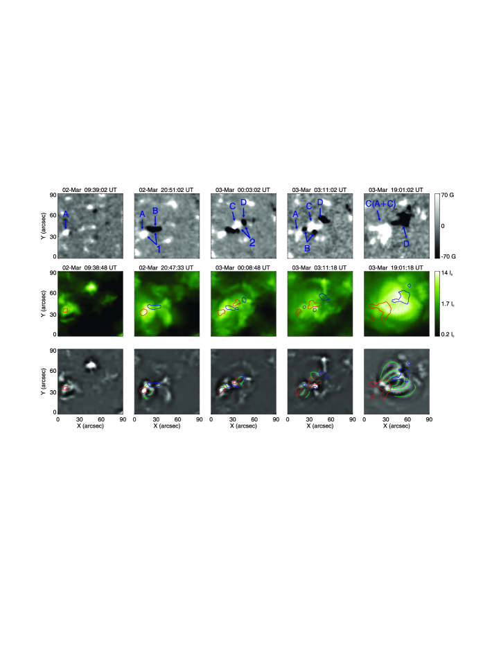
Figure 2: Interaction between two dipoles. From top to bottom: MDI magnetograms, EUVI 171 Å images and corresponding contrast enhanced images. Red and blue curves are contours of the positive ($+$70 G) and negative ($-$70 G) magnetic fields, while green curves emphasize and figure out loop connections. Arrows “1” and “2” denote two dipoles emerging one after the other. We denote the positive and negative elements of dipole “1” (“2”) with arrows “A” and “B” (“C” and “D”), respectively.

Figure 2 presents the interaction process between the two dipoles. Top panels are time sequence of MDI magnetograms, which show the emergence and interaction of the two dipoles. The middle panels exhibit the coronal response in EUVI 171 Å line. Loop connections can be seen much more clearly in the contrast enhanced 171 Å images (bottom panels). The positive element “A” of the first dipole (denoted by arrows “1”) appeared obvious at 09:39 UT 02 March and then grew larger, and brightening point appeared simultaneously at the corresponding location as shown in the leftmost column. Then the negative element “B” began to emerge and the dipole “1” reached its maximum size with total unsigned LOS flux of 2.0$\times 10$²⁰ Mx at 20:51 UT 02 March. At this time, the loop connections between elements “A” and “B” are emphasized with green curves in the contrast enhanced image at 20:47 UT 02 March. The second dipole (indicated by arrows “2”) started to appear in the magnetogram from 20:51 UT 02 March with slightly distinguishable features and became quite obvious at 22:27 UT 02 march. The magnetogram acquired at 00:03 UT on 03 March shows that its positive element “C” was located in contact with element “B”. Element “B” split into two segments during its disappearance process, as shown in the magnetogram at 03:11 UT 03 March. Both two segments of “B” disappeared completely at 08:22 UT 03 March. Element “A” moved toward “C” and merged with “C” into “A$+$C”, still called element “C” by us considering the small size of “A” compared to that of “C”. Dipole “2” continued emerging and reached its maximum with total unsigned LOS flux of 9.8$\times 10$²⁰ Mx at 19:01 UT 03 March (top right panel).

During the interaction process between the two dipoles, a jet and a plasma eruption have been observed, as shown in Fig. 3. At the early emerging stage of the dipole “2”, there was a small bright point (denoted by arrow “1”) at the adjacent area of elements “B” and “C” (top left panel). Two and a half minutes later, a jet (indicated by arrows “2”) rooting at the bright point was observed. The lifetime of the jet is only 5 minutes. The second dipole continued to emerge and another obvious brightening point (indicated by arrow “3”) appeared at the contacted region of “B” and “C” (bottom left panel). At 23:46 UT, a cloud of plasma was disturbed (denoted by arrow “a”) and erupted five minutes later (arrow “b”). After the eruption, a dimming area appeared (arrow “c”).

4.2 Magnetic flux cancellation of the second dipole

Two elements of dipole “2” separated as flux continually emerged until 19:01 UT 03 March. Then they began to cancel with each other, as shown in Fig. 4. Top five panels display the evolution of dipole “2” in five days. When the dipole well developed, the flux of each polarity was almost concentrated. As the cancellation began, each pole broke into several fragments. Then these fragments with opposite polarities moved together and cancelled gradually. Accompanying the cancellation process, the corresponding coronal region in 171 Å images became darker (middle panels), while the general loop connections were not changed much (bottom panels). However, the loop systems became fewer and fuzzier, and the length of loops became shorter. At 20:47 UT 03 March, the amount of identifiable loops was 7 while there was no more than 4 at 06:23 UT 05 March. At 19:01 UT 03 March, when the dipole well developed, the length of the longest loop was about 30 Mm. Two days later, most of the long coronal loops were about 15 Mm. At 06:24 07 March, only small dispersed elements of dipole “2” remained (bottom right panel in Fig. 1). The northeastern part of the CH, where the dipoles were located, appeared as a quiet region and the underlying magnetic fields evolved to mixed polarities (see the rectangle region in Fig. 1).

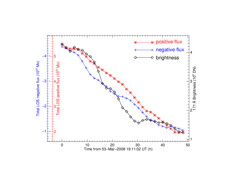
Figure 5: Temporal variations of negative and positive magnetic flux in MDI magentograms and brightness in 171 Å images derived from the ellipse region in Fig. 4.

Figure 5 shows the temporal variations of negative and positive magnetic flux in MDI magnetograms and brightness in 171 Å images obtained from the ellipse region in Fig. 4. In two days, both the negative and positive flux reduced smoothly by 3.4$\times$10²⁰ Mx at a steady cancellation rate of 0.7$\times$10¹⁹ Mx h^-1. During this period, the brightness in 171 Å images decreased by about 75%.

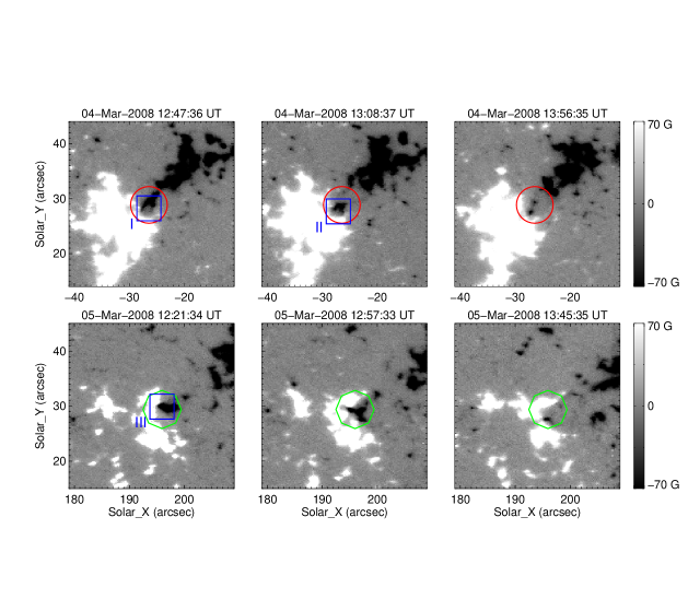
Figure 6: Time sequence of Hinode$/$NFI Na V/I magnetograms displaying magnetic flux cancellation. Circles and octagons show two cancellation events on two days, respectively. Rectangles “I” “II” and “III” outline the locations of SP maps from top to bottom in Fig. 8.

The Na V/I high spatial resolution magnetograms are used to study the cancellation between two polarities of dipole “2” in details. Two obvious cancellation processes are displayed in Fig. 6. In the circle region (top panels), a negative flux island moved straightly toward the positive flux, cancelled with it and disappeared totally at 14:29 UT 04 March. In the octagon area (bottom panels), another flux island observed on 05 March also cancelled with the positive flux. We measure the cancellation rates between the opposite polarities of the second dipole in the calibrated Na V/I magnetograms (within the rectangle area outlined in Fig. 4). It indicates that both the positive and negative polarities decreased at an average rate of 0.8$\times$10¹⁹ Mx h^-1 during the period of 11:20–16:17 on 04 March and of 0.7$\times$10¹⁹ Mx h^-1 from 11:39 to 15:27 on 05 March. We also measure the disappearing rate of the two small negative islands shown in Fig. 6. At the pre-cancellation stage, the flux of the two islands is $-$0.4$\times$10¹⁹ Mx (outlined with circles in the top panels) and $-$0.5$\times$10¹⁹ Mx (outlined with octagons in the bottom panels), respectively. Both the two islands disappeared at a mean rate of 0.3$\times$10¹⁹ Mx h^-1.

The negative island shown in the circle region in Fig. 6 moved toward the positive island during its cancellation course. Its distance from the initial site and apparent horizontal velocity at different time are presented in Fig. 7. The average horizontal velocity is 1.0 km s^-1. Although the V/I magnetograms have been coaligned with the cross-correlation method, there still exists an uncertainty in determining the magnetic island position. A position error (one pixel) introduces an error of the velocity of (one pixel)/(time interval). In order to reduce the velocity error, we measure the island position every 6 minutes. As the size of one pixel is 0″.16 and the time interval is 6 minutes, the error becomes 0.3 km s^-1.

Hinode$/$SP also observed the cancellation regions. The vector magnetic fields and Doppler velocities derived from the SP data help us to investigate the physical essence of magnetic field evolution at the cancellation sites. Figure 8 shows the appearance of three cancellation stages in small sub-regions observed with SP. From left to right: longitudinal fields ($\alpha_{mag}Bcos\gamma$), transverse fields ($(\alpha_{mag})^{1/2}Bsin\gamma$), inclinations ($\gamma$) and Doppler velocities ($V_{los}$). Top panels show the properties of four parameters at the cancellation area at 11:24 UT 04 March. In the longitudinal magnetogram (top left panel), the cancellation takes place at the area between the positive and negative elements (outlined by the parallelogram), and the transverse fields are strong and point directly from the positive island to the negative one (second panel). The third panel shows magnetic field inclinations where the black areas (inclination of 90$\arcdeg$) indicate horizontal orientations and white areas (0$\arcdeg$ and 180$\arcdeg$) vertical ones. At the polarity inversion line (dotted curve), the magnetic fields are nearly horizontal. Within the parallelogram region in the Dopplergram (top right panel), larger Doppler red-shifts with a mean downward velocity of 1.15 km s^-1 are observed. The second and third rows exhibit other two cancellation stages similar to the first one, and the average Doppler velocities within the parallelogram regions are 0.84 km s^-1 and 0.70 km s^-1, respectively.

5 Conclusions and discussion

Using coordinated SOHO, STEREO and Hinode observations, we investigate the evolution of two dipoles in a CH region. The negative element of the first dipole disappears due to its interaction with the positive element of the second dipole. During this process, a jet and a plasma eruption are observed. Two opposite poles of the second dipole constantly emerge and separate at first, and then cancel with each other. With the decrease of magnetic flux caused by cancellation, the brightness in 171 Å images decreases and coronal loops shrink obviously. At the cancellation sites of the second dipole, the transverse fields are strong and point directly from the positive elements to the negative ones. Larger Doppler red-shifts are also observed between the cancelling elements. At last, the northeastern part of the CH, where the dipoles are located, appears as a quiet region.

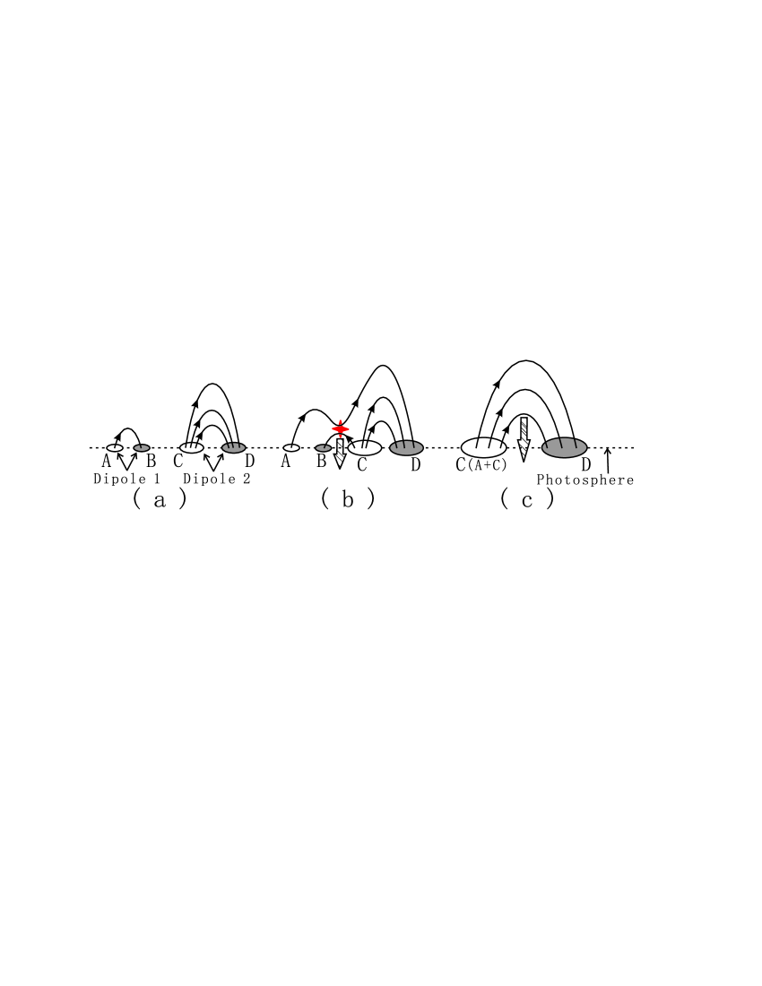
Figure 9: Cartoons illustrating evolution process of the two dipoles. (a) Pre-interaction state of the dipoles. (b) Flux disappearance due to reconnection accompanied with energy release. (c) Flux cancellation caused by submergence of original loops connecting the dipolar elements. “A” and “B” (“C” and “D”) represent the positive and negative elements of dipole “1” (“2”), respectively. Asterisk marks magnetic flux reconnection and cross hatched arrows indicate flux submergence.

Based on the observational results in this study, we consider that the interaction between the two dipoles is caused by flux reconnection, while that between the opposite polarities of the second dipole is due to the submergence of original loops. This phenomenon is first reported in a CH. To illustrate the evolution process of the two dipoles, a series of cartoons are sketched out (see Fig. 9). Dipole “1” appears first and dipole “2” emerges later at the adjacent area of dipole “1” (Fig. 9a). We mark the positive and negative elements of dipole “1” (“2”) with “A” and “B” (“C” and “D”), respectively. Magnetic flux reconnection occurs between two groups of loops connecting the opposite polarities. Magnetic loops are restructured to a configuration of lower potential energy accompanied with energy release. Meanwhile, small loops form and submerge, leading to an observational phenomenon, magnetic flux cancellation. Element “B” totally disappears due to the cancellation with part of element “C”. Two poles “C” and “D”, which are originally connected by flux loops, draw back and cancel with each other due to flux submergence (Fig. 9c).

Observational evidences, e.g. the jet and the plasma eruption exhibited in Fig. 3 indicate that the interaction between elements “B” and “C” represents a flux reconnection process. When magnetic reconnection occurs, magnetic energy is converted into thermal energy and kinetic energy. Then plasma jet forms and ejects along the field line (Yokoyama & Shibata 1995). Accompanying the reconnection, plasma eruption may also be formed due to the change of magnetic configuration. However, we can not absolutely rule out the possibility that the disappearance of element “B” is caused by the emergence of U$-$shaped magnetic loops connecting “B” and “C” from below the photosphere (Parker 1984; Lites et al. 1995), for we lack more relevant observational information.

Flux loops are always affected by magnetic buoyancy and tension of subsurface field lines. When the tension gains the upper hand, the flux loops are pulled back down by magnetic tension and submerge (Zirin 1985). The movies of 1-min cadence MDI magnetograms and 3-min cadence Na V/I magnetograms and the results revealed in Figs. 4$-$8 let us believe that the cancellation between “C” and “D” is caused by the submergence of original loops. From Fig. 7, we obtain an average horizontal velocity of 1.0 km s^-1. When we assume flux loops connecting the cancelling elements are approximately semicircular, the vertical velocity of submergence is 1.0 km s^-1. At the cancellation sites in this study, we observe a mean downward velocity of 0.9 km s^-1 (averaging the values of 1.15 km s^-1, 0.84 km s^-1 and 0.70 km s^-1 in the three stages), much higher than that of the surrounding areas (Fig. 8), comparable to the velocity obtained from the cancelling flux motion in Fig. 7 (1.0 km s^-1) and consistent with the velocities reported by Harvey et al. (1999) (0.3$-$1.0 km s^-1) and Chae et al. (2004) (1.0 km s^-1).

Evolution of CHs refers to several aspects, such as CH formation and decay, and the temporal variation of CH boundary. The key quantity for understanding these aspects is magnetic field. Magnetic flux emergence, cancellation, mergence and dispersion are the main forms of magnetic field evolution. They are all found in the dipolar evolution process in the CH in this study. An interesting cancelling form, i.e. submergence of initial loops after emergence, is also observed for the first time in the CH. At the late stage of the dipolar evolution, the area where the dipoles are located becomes mixed polarities instead of unipolar fields, resulting in the change of the overlying corona from a CH area to a quiet region (see the rectangle region in Fig. 1). This confirms the result of Zhang et al. (2007) that one of the signatures of decay of a CH is the disappearance of the magnetic flux imbalance. These results enlighten us that, in order to understand the CH evolution, it is important to study magnetic field evolution in CHs. In particular, to investigate the evolution of dipoles may be an efficient approach to understand CH decay and disappearance.

Table 1: Data sets used in this study.

Observation	Period	Cadence	Pixel Size	Field of View
	(UT)	(minutes)	(arcsec)	(arcsec2)
SOHO$/$MDI	02 08:03 – 07 12:47	96	1.97	full disk
	02 11:35 – 02 14:36	1	1.97	full disk
	03 00:57 – 07 12:00	1	1.97	full disk
SOHO$/$EIT(195Å)	02 08:00 – 07 12:00	12	2.63	full disk
STEREO-B$/$EUVI(171Å)	02 08:00 – 05 00:00	2.5	1.59	full disk
STEREO-A$/$EUVI(171Å)	05 00:00 – 07 12:00	2.5	1.59	full disk
Hinode$/$SP(Fe full Stokes)	03 12:00 – 14:42	50	0.32	59.04${\times}$162.30
	04 11:20 – 15:55	50	0.32	59.04${\times}$162.30
	05 11:40 – 15:15	45	0.32	59.04${\times}$162.30
Hinode$/$NFI(Na Stokes I, V)	03 10:53 – 15:27	3	0.16	163.84${\times}$163.84
	04 11:20 – 16:17	3	0.16	64.00${\times}$163.84
	05 11:39 – 15:27	3	0.16	64.00${\times}$163.84

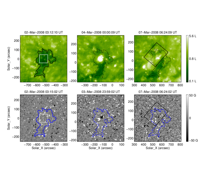
Figure 1: EIT 195 Å images (top panels) and MDI magnetograms (bottom panels) showing the evolution of the CH. Black and blue curves delineate the CH boundary derived from the EUVI 284 Å image obtained at 03:06:30 UT 02 March 2008. The squares outline the field-of-view of Figs. 2$-$4 and rectangles enclose a QS region.

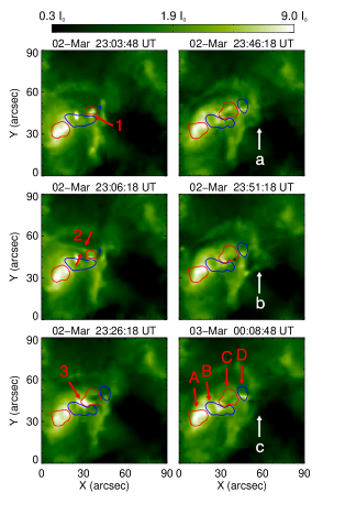
Figure 3: EUVI images displaying a jet and a plasma eruption. “A”–“D” are contours of two dipoles at $\pm$30 G levels from MDI magnetogram at 22:27 UT 02 March (first two panels) and at 00:03 UT 03 March (other panels). Arrows “1” and “3” denote two brightening points, while arrows “2” indicate an EUV jet. Arrows “a”–“c” show the different stages of a plasma eruption.

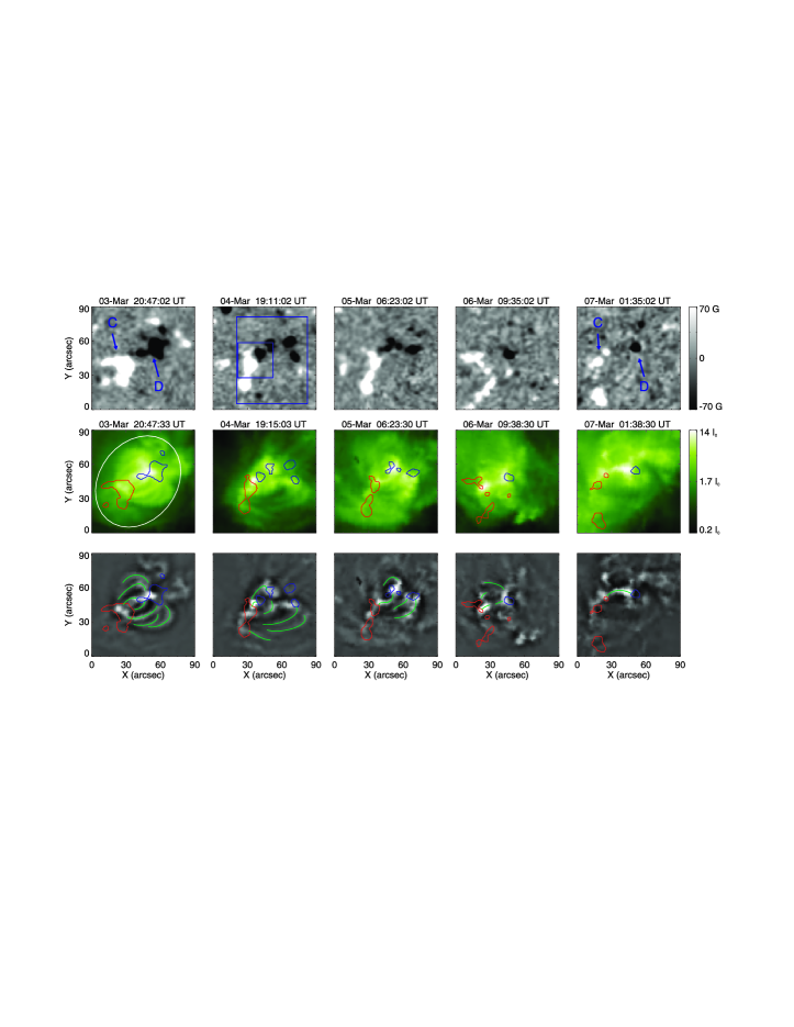
Figure 4: Similar to Fig. 2 but for magnetic flux cancellation between two polarities of dipole “2”. Small square on the second MDI magnetogram outlines the field-of-view of Fig. 6 and larger rectangle the area where the positive and negative flux of the second dipole are measured in the Na V/I magnetograms. Ellipse outlines the region where magnetic flux in MDI magnetograms and brightness in 171 Å images are measured.

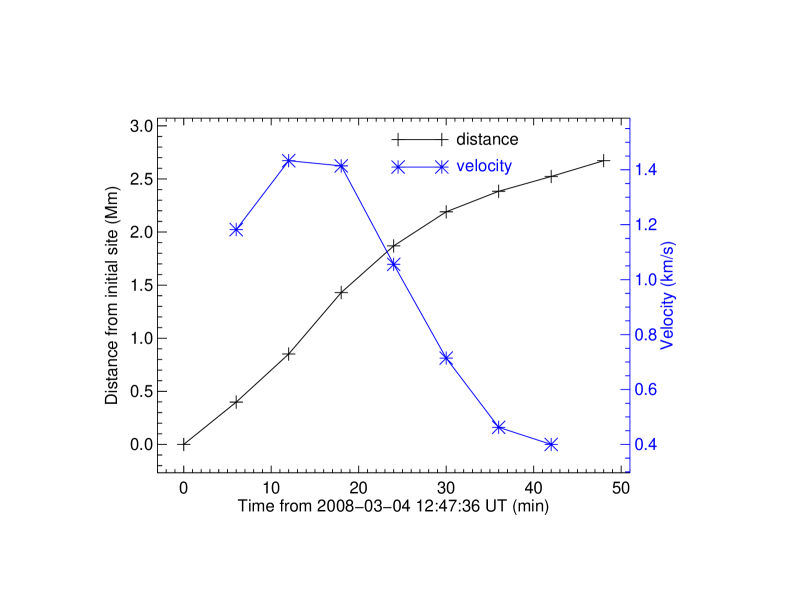
Figure 7: Temporal variations of distance and apparent horizontal velocity of the negative island in the circle region shown in Fig. 6.

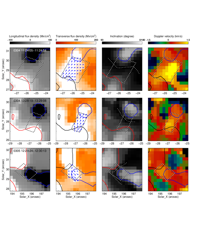
Figure 8: Appearance of cancellation regions observed by Hinode$/$SP. From left to right: longitudinal fields, transverse fields, inclinations and Doppler velocities. Inclinations of 90$\arcdeg$ correspond to magnetic fields with horizontal orientations, and positive Doppler velocities to red-shifts. Blue curves are contours of negative elements ($-$100 G) and other solid curves outline the positive ones (+100 G). Dotted curves represent the polarity inversion lines. Arrows denote the transverse fields and parallelograms outline the areas where cancellations take place.

References

- (1) Bohlin, J. D. 1977, Sol. Phys., 51, 377
- (2) Borrero, J. M., Tomczyk, S., Kubo, M., et al. accepted for publication in Sol. Phys., eprint arXiv: 0901.2702
- (3) Brault, J., & Neckel, H. 1987, Spectral atlas of the solar absolute disk-averaged and disk center intensity from 3290 Å to 12510 Å available at ftp.hs.uni-hamburg.de/pub/outgoing/FTS-atlas
- (4) Chae, J., Moon, Y., Park, Y., et al. 2007, PASJ, 59, S619
- (5) Chae, J., Moon, Y., & Pevtsov, A. A. 2004, ApJ, 602, L65
- (6) Chiuderi Drago, F., Landi, E., Fludra, A., & Kerdraon, A. 1999, A&A, 348, 261
- (7) Danilovic, S., Gandorfer, A., Lagg, A., et al. 2008, A&A, 484, L17
- (8) Delaboudinière, J. P., Artzner, G. E., Brunaud, J., et al. 1995, Sol. Phys., 162, 291
- (9) Domingo, V., Fleck, B., & Poland, A. I. 1995, Sol. Phys., 162, 1
- (10) Feng, L., Inhester, B., Solanki, S. K., et al. 2007, ApJ, 671, L205
- (11) Fisk, L. A. 2005, ApJ, 626, 563
- (12) Fisk, L. A., & Schwadron, N. A. 2001, ApJ, 560, 425
- (13) Harvey, K. L. 1996, in AIP Conf. Ser. 382, Proc. Eighth International Solar Wind Conference, ed. D. Winterhalter et al. (New York: AIP), 9
- (14) Harvey, K. L., Jones, H. P., Schrijver, C. J., & Penn, M. J. 1999, Sol. Phys., 190, 35
- (15) Harvey, K. L., & Recely, F. 2002, Sol. Phys., 211, 31
- (16) Howard, R. A., Moses, J. D., Vourlidas, A., et al. 2008, Space Sci. Rev., 136, 67
- (17) Ichimoto, K., Lites, B., Elmore, D., et al. 2008, Sol. Phys., 249, 233
- (18) Kaiser, M. L., Kucera, T. A., Davila, J. M., et al. 2008, Space Sci. Rev., 136, 5
- (19) Kano, R., & Tsuneta, S. 1995, ApJ, 454, 934
- (20) Kosugi, T., Matsuzaki, K., Sakao, T., et al. 2007, Sol. Phys., 243, 3
- (21) Krieger, A. S., Timothy, A. F., & Roelof, E. C. 1973, Sol. Phys., 29, 505
- (22) Kubo, M., Lites, B. W., Ichinoto, K., Shimizu, T., et al. 2008, ApJ, 681, 1677
- (23) Kubo, M., & Shimizu, T. 2007, ApJ, 671, 990
- (24) Levine, R. H. 1977, ApJ, 218, 291
- (25) Liggett, M. & Zirin, H. 1983, Sol. Phys., 84, 3
- (26) Lites, B. W., Elmore, D. F., & Streander, K. V. 2001, in ASP Conf. Ser. 236, Advanced Solar Polarimetry-Theory, Observation, and Instrumentation, ed. M. Sigwarth (San Francisco: ASP), 33
- (27) Lites, B. W., Low, B. C., Martinez Pillet, V., et al. 1995, ApJ, 446, 877
- (28) Livi, S. H. B., Wang, J., & Martin, S. F. 1985, Australian J. Phys., 38, 855
- (29) Luo, B. X., Zhong, Q. Z., Liu, S. Q., & Gong, J. C. 2008, Sol. Phys., 250, 159
- (30) Martin, S. F., Livi, S. H. B., & Wang, J. 1985, Australian J. Phys., 38, 929
- (31) Munro, R. H., & Withbroe, G. L. 1972, ApJ, 176, 511
- (32) Orozco Suárez, D., Bellot Rubio, L. R., Del Toro Iniesta, J. C., et al. 2007, ApJ, 670, L61
- (33) Parker, E. N. 1984, ApJ, 280, 423
- (34) Rabin, D., Moore, R., & Hagyard, M. J. 1984, ApJ, 287, 404
- (35) Reeves, E. M., & Parkinson, W. H. 1970, ApJS, 21, 1
- (36) Scherrer, P. H., Bogart, R. S., Bush, R. I., et al. 1995, Sol. Phys., 162, 129
- (37) Shen, C. L., Wang, Y. M., Ye, P. Z., & Wang, S. 2006, ApJ, 639, 510
- (38) Shimizu, T., Nagata, S., Tsuneta, S., et al. 2008, Sol. Phys., 249, 221
- (39) Suematsu, Y., Tsuneta, S., Ichimoto, K., et al. 2008, Sol. Phys., 249, 197
- (40) Tsuneta, S., Ichimoto, K., Katsukawa, Y., et al. 2008, Sol. Phys., 249, 167
- (41) Tu, C. Y., Zhou, C., Marsch, E., et al. 2005, Science, 308, 519
- (42) Underwood, J. H., & Muney, W. S. 1967, Sol. Phys., 1, 129
- (43) Wallenhorst, S. G., & Topka, K. P. 1982, Sol. Phys., 81, 33
- (44) Wang, Y. M., Hawley, S. H., & Sheeley, N. R. 1996, Science, 271, 464
- (45) Wiegelmann, T., & Solanki, S. K. 2004, Sol. Phys., 225, 227
- (46) Yokoyama, T., & Shibata, K. 1995, Nature, 375, 42
- (47) Yurchyshyn, V. B., & Wang, H. 2001, Sol. Phys., 202, 309
- (48) Zhang, J., Ma, J., & Wang, H. M. 2006, ApJ, 649, 464
- (49) Zhang, J., Wang, J., Deng, Y., & Wu, D. 2001, ApJ, 548, L99
- (50) Zhang, J., Yang, S. H., & Jin, C. L. 2009, eprint arXiv: 0905.1553
- (51) Zhang, J., Zhou, G. P., Wang, J. X., & Wang, H. M. 2007, ApJ, 655, L113
- (52) Zirin, H. 1985, ApJ, 291, 858
- (53) Zirker, J. B., ed. 1977, Coronal Holes and High-Speed Wind Streams (Boulder: Colorado Associated Univ. Press)
- (54) Zwaan, C. 1978, Sol. Phys., 60, 213
- (55) Zwaan, C. 1987, ARA&A, 25, 83