Geometric scaling in the spectrum of an electron
captured by a stationary finite dipole

Abstract

We examine the energy spectrum of a charged particle in the presence of a non-rotating finite electric dipole. For any value of the dipole moment $p$ above a certain critical value $p_{\mathrm{c}}$ an infinite series of bound states arises of which the energy eigenvalues obey an Efimov-like geometric scaling law with an accumulation point at zero energy. These properties are largely destroyed in a realistic situation when rotations are included. Nevertheless, our analysis of the idealised case is of interest because it may possibly be realised using quantum dots as artificial atoms.

1 Introduction

The problem of a charged particle in the field of a physical electric dipole serves as the starting point for the description of a variety of important physical processes, ranging from e.g., the passage of muons through a substance [1], the determination of carrier mobilities and charge trapping states in various condensed matter systems [2, 3], to the chemical bonding of two atoms [4, 5]. Despite the vast amount of literature on the quantum mechanics of this system, there have been remarkably few detailed, numerically exact studies [6, 7]. Past efforts have focused on the narrow region near criticality where scattering states from the continuum are brought down into the discrete spectrum [8, 9, 10, 11]. The primary impetus for these studies is rooted in chemistry where the determination of the critical dipole moment(s), along with the binding energy of the charged particle, are very important. It is well established that a non-rotating, rigid dipole can only bind a charged particle if the dipole moment exceeds the critical $p_{\mathrm{c}}\approx 1.6249$ Debye.

While part of the reason for the heretofore limited numerical results can be attributed to the computationally intensive nature of the calculations, the more significant issue has likely been the absence of additional physical motivation to warrant further studies. It is now known that the inclusion of rotation drastically alters the idealised spectrum[12, 13] of the stationary dipole. With the advent of quantum dots as artificial atoms, however, there is a possibility that the rotational degrees of freedom are irrelevant. In that case the idealised model of this paper may be of interest to the ultra-cold atoms community, who look for such a spectrum at Efimov resonance [14, 15].

In this Letter, we present a detailed, numerically exact investigation for the bound-state energy spectrum of a charged particle in the field of a stationary finite dipole. This model occurred in the physics literature as early as 1947 [1]. It was firmly established and later “rediscovered” [16] that a finite stationary dipole can capture an electron if the dipole moment, $p$, is larger than a critical value $p_{c}$. Furthermore, for supercritical values of $p$ not only one but infinitely many bound state appears in the spectrum, with an accumulation point at $E=0$.

We focus our attention on the same system: a rigid, stationary dipole, hence we exclude the effect of rotation of the dipole from our calculation. Nevertheless we have to note that rotation may play an important role in influencing the spectrum of the electron, especially if the moment of inertia, $I$, of the dipole is small. Garrett [12, 13] showed that the critical dipole moment, $p_{c}$, is larger compared to that of a stationary dipole and depends on $I$. Additionally, for $p>p_{c}$ the number of bound states is reduced to a finite value and the infinitude of the number of bound states is only recovered if $I\rightarrow\infty$.

Until now the striking similarity between the detailed spectrum of our system and the three-body Efimov levels [17, 18] has not been emphasised. Despite the different origins of these two effects [19], our numerical and analytical results of the bound electronic spectrum for $p>p_{c}$ yield two features that resemble an Efimov-spectrum:

• a geometric scaling law of consecutive binding energies, $E_{n+1}/E_{n}={\mathrm{constant}}$, and

• an accumulation of the bound states as $E\rightarrow 0^{-}$.

Figure 1: Schematic representation of the model. The line joining the center of the dipole to $q_{e}$ is of length $r$, and makes an angle $\theta$ with the $z$-axis.

2 The model

Our physical model consists of three charged particles as schematically illustrated in figure 1. We keep the position of two particles fixed (i.e., $Q_{1}$ and $Q_{2}$) and look for the bound state(s), if such exists, of the third particle. Specifically, for the stationary rigid dipole, we choose $Q_{1}=-Q_{2}=Q$, and the third particle is taken to be an electron. Therefore the Hamiltonian, $\mathbf{H}$, for our system reads

$$\mathbf{H}=-\frac{\hbar^{2}}{2m_{e}}\nabla^{2}+\frac{Qq_{e}}{4\pi\epsilon_{0}}\left(\frac{1}{\left|{\mathbf{r}}_{1}\right|}-\frac{1}{\left|{\mathbf{r}}_{2}\right|}\right)~{}.$$ (1)

It is convenient to introduce the dimensionless dipole moment, $\lambda$, with the definition

$$\lambda=\frac{2m_{\mathrm{e}}}{\hbar^{2}}\ \frac{pq_{\mathrm{e}}}{4\pi\epsilon_{0}}~{},$$ (2)

where $p$ denotes the electric dipole moment, $p=Qd$, and $d$ is the size of the physical dipole. Finally, scaling all lengths as ${\mathbf{r}}_{i}\rightarrow{\mathbf{r}}_{i}/d$, reduces eq. (1) to

$$\mathbf{H}=-\nabla^{2}+{\lambda}\left(\frac{1}{\left|{\mathbf{r}}_{1}\right|}-\frac{1}{\left|{\mathbf{r}}_{2}\right|}\right)~{}.$$ (3)

In our simplified picture, $\lambda$ characterises the strength of the interaction between the originally unbound electron and the physical dipole. If $\lambda$ does not exceed the threshold value $\lambda_{c}\approx 1.27863$, the third particle cannot be bound. The minimum $\lambda$ then represents the critical strength at which the first zero-energy bound state appears. Note, from eq.  (3), that for $r\gg d$, the potential goes like $\cos{\!(\theta)}/r^{2}$ in spherical polar co-ordinates, where $r$ and $\theta$ are defined in figure 1. For $r\ll d$, however, the potential has no singularity, and goes to zero as $r\rightarrow 0$. At threshold, the spatial extent of the wavefunction for the third particle becomes much greater than the size of the dipole [20], and the short-distance length scale, $d$, set by the size of the dipole may be ignored. As a result, the same critical value $\lambda_{c}$ is obtained for both the finite and for the point dipole [21, 22, 23, 24]. For $p>p_{c}$, however, the point dipole potential $\cos{\!(\theta)}/r^{2}$ has no lower bound in energy because of the $r^{-2}$ singularity at the origin [23], and is unphysical. By contrast, our finite-sized dipole potential is well-behaved for all r, thereby yielding a meaningful bound state spectrum for $p>p_{c}$. Moreover, it is the inverse-square nature of this potential for large distances that gives rise to the Efimov-like features of the spectrum [25].

Numerical implementation — The bound state energies, $E<0$, and wavefunction, $\Psi$, for the electron are obtained from the reduced Schrödinger equation,

$$\mathbf{H}\Psi=-\kappa^{2}\Psi,$$ (4)

where $\kappa^{2}=-2m_{e}Ed^{2}/\hbar^{2}\geq 0$ is the dimensionless energy. Equation (4) is separable in prolate spheroidal coordinates [26], resulting in the following equations ($\varphi\in[0,2\pi[$, $\xi\in[1,\infty[$ and $\eta\in[-1,1]$)

$$\frac{dF}{d\varphi}+m^{2}F=0$$ (5a)

$$\frac{d}{d\xi}\!\left[(\xi^{2}-1)\frac{dS}{d\xi}\right]+\!\left[-A+\kappa^{2}\xi^{2}-\frac{m^{2}}{\xi^{2}-1}\right]S=0$$ (5b)

$$\frac{d}{d\eta}\!\left[(1-\eta^{2})\frac{dT}{d\eta}\right]+\!\left[A-\lambda\eta-\kappa^{2}\eta^{2}-\frac{m^{2}}{1-\eta^{2}}\right]T=0$$ (5c)

where the wavefunction has been factorised as $\Psi=S(\xi)T(\eta)F(\varphi)$. The reduction of the three-dimensional Schrödinger equation to a set of three one-dimensional ordinary differential equations (ODEs) requires the appearance of two separation constants, $A$ and $m$. Separability, as the manifestation of a symmetry, also means here that these constants are the eigenvalues of conserved quantities [27, 28]. If there is no electric dipole, i.e. $\lambda=0$, the electron is free and the solution of the original physical problem is known. In this case the two conserved quantities are $\mathbf{L}^{2}$ and $\mathbf{L}_{z}$ with eigenvalues $\ell(\ell+1)$ and $m$, where $\ell$=0,1,…and $m=$0, $\pm$1, …$\pm\ell$. Since our potential does not possess spherical symmetry for $\lambda>0$, the ($2\ell+1$) degeneracy of $m$ is absent, although the azimuthal symmetry of the finite dipole still guarantees the conservation of $\mathbf{L}_{z}$. Notice that the same is not true for $\mathbf{L}^{2}$, therefore $\ell$ is no longer a good quantum number. In what follows, we adopt the notation established previously in the literature [6, 29, 7] and label the energy eigenvalues of $\mathbf{H}$ by a set of three numbers ($n_{\xi}$, $n_{\eta}$, $m$) where $n_{\xi}$ counts the zeros of $S(\xi)$, while $n_{\eta}$ does so for $T(\eta)$.

Although the general solution of the above equations can be analytically given in terms of double-confluent Heun functions [30], this approach does not offer a feasible way for deriving the energy eigenvalues explicitly. Consequently, we fall back to numerical methods [31, 32] for finding normalisable solutions to these equations for a given value of $\lambda$ and $\kappa^{2}$.

In the first instance, we assume that the separation constant $A$ can be different in the two equations. In this way we obtain two sets of curves, viz. $\kappa^{2}$ vs. $A_{\mathrm{rad}}$ and $A_{\mathrm{ang}}$, for the radial (5b) and for the angular equation (5c), respectively. Only the latter curve, $A_{\mathrm{ang}}$, depends on the dimensionless dipole moment $\lambda$, since $\lambda$ is present in (5c), but absent in (5b). The crossing(s) of these two sets of curves represents the desired solution to the system of ODEs since the separation constant $A=A_{\mathrm{rad}}=A_{\mathrm{ang}}$ and $\kappa^{2}$ become common for the two equations.

Figure 2 shows the two sets of curves, $A_{\mathrm{rad}}$ and $A_{\mathrm{ang}}$ for $\lambda\equiv 0$, which case represents a free electron, therefore $\mathbf{L}^{2}$ is conserved and $\ell$ is a good quantum number to label the curves with. The fan structure of $A_{\mathrm{ang}}$ is apparent in the figure and remains intact for non-vanishing dipole moments. For $0<\lambda<\lambda_{\mathrm{c}}$, there is no common point for the two sets of curves in the $\kappa^{2}>0$ domain, thus no bound state exists. On one hand, it can also be proven, that $\lim_{\kappa^{2}=0^{+}}{\left(A_{\mathrm{rad}}\right)}=-1/4$, i.e. all $A_{\mathrm{rad}}$ curves approach the value ($-1/4$). On the other hand as we increase the dipole moment the $A_{\mathrm{ang}}$ curves shift towards left (see fig. 3). Therefore there must be a critical value of the dimensionless dipole moment $\lambda$ at which the first $A_{\mathrm{ang}}$ curve, labelled by ($n_{\eta}=0,m=0$), also crosses the abscissa at ($-1/4$). However, above this critical value of $\lambda$, $A_{\mathrm{ang}}$(0,0) crosses infinitely many curves of $A_{\mathrm{rad}}$; this is the mathematical origin of the infinite “tower” of bound states if $\lambda\geq\lambda_{\mathrm{c}}$. Figure 3 depicts $A_{\mathrm{ang}}(n_{\eta},m)$ only for $(n_{\eta}=0,m=0)$. Increasing $\lambda$ further, more and more branches of the “fan” are shifted to the left and cross the value ($-1/4$), hence one can deduce a critical value of $\lambda$ for each “tower” labelled by $(n_{\eta},m)$. The value of the five lowest $\lambda_{c}(n_{\eta},m)$ are reported in table 1. As $\lambda$ exceeds a given $\lambda_{c}(n_{\eta},m)$ a new “tower” of infinitely many bound states opens, e.g. for $\lambda=16$ there will be three sets, ($n_{\eta},m$) = (0,0), (0,1) and (1,0) each containing infinitely many bound states labelled by $n_{\xi}=$0, 1, 2, …

The values of $A_{\mathrm{ang}}$ and $A_{\mathrm{rad}}$ are calculated as eigenvalues of matrices or from three-term recursions [31, 32]. Numerically, it is demanding to obtain precise values for the crossings, particularly for the rapidly decaying $A_{\mathrm{rad}}$ curves near the critical region $\lambda\rightarrow\lambda_{\mathrm{c}}^{+}$.

Figure 2: The angular (thin lines) and radial (thick lines) separation constants (5b-c) are plotted versus the dimensionless energy eigenvalue $\kappa^{2}$ for $\lambda=0$. Each curve of $A_{\mathrm{ang}}$, except the ones for $m=0$, is doubly degenerate, therefore each branch originating from $\ell(\ell+1)$ has ($2\ell+1$) curves altogether. The curves of the radial separation constant are labelled by ($n_{\xi}$, $m=0$). If $\lambda<\lambda_{\mathrm{c}}$ there is no crossing at positive $\kappa$, and there is no bound state.

Figure 3: The angular (thin line) and radial (thick line) separation constants are plotted versus the dimensionless energy eigenvalue $\kappa^{2}$. The curves of the radial separation constant are labelled by ($n_{\xi}$, $m=0$). Their rapid decrease as energy approaches zero is apparent. Moreover, figure shows only ($n_{\eta}=0$, $m=0$) angular separation constant for four different $\lambda$ values: two below the critical value, one at the critical value ($\approx$ 1.2786) and one much larger than the critical value. The small vertical arrow at $A_{\mathrm{rad}}=A_{\mathrm{ang}}=-1/4$ captures the position where the zero-energy bound states first appear.

3 Results

For a given set of $(n_{\eta},m)$, if $\lambda\geq\lambda_{\mathrm{c}}(n_{\eta},m)$ there are an infinite tower of bound states, irrespective of the value of $\lambda$. This result is in marked contrast to what is found in the Efimov effect, where the infinite tower of bound states for the three-body system occurs only at criticality. We note that the lowest critical dipole moment $\lambda_{\mathrm{c}}\approx 1.2786$ corresponds to an electron with quantum numbers (0,0,0), that gives a zero-energy bound state. For $n_{\eta}>0$, it is well-known in the literature that higher values of $\lambda_{c}$ are needed. Our exact numerical results (see Table 1) confirm these super-critical values [24] with high accuracy.

Table 1: The five lowest values of $\lambda_{\mathrm{c}}(n_{\eta},m)$ are given. If $\lambda>\lambda_{\mathrm{c}}(n_{\eta},m)$ a new set of infinite set of bound states is created.

$n_{\eta}$	$m$	$\lambda_{\mathrm{c}}$		$p_{\mathrm{c}}$ (Debye)
0	0	1.2786298		1.625
0	1	7.5839359		9.638
1	0	15.0939114		19.182
0	2	19.0580547		24.220
1	1	28.2242292		35.869

Figure 4 summarises the central results of this paper. Focusing first on the curves with symbols, the main figure shows the ratio of consecutive bound state energies for a variety of dimensionless dipole moments. It is evident that at criticality, $\lambda=\lambda_{\mathrm{c}}$, the ratio diverges, which is expected given that this is the dipole moment for which the zero energy state appears. In addition, we see that above criticality, the ratio $\gamma$, decays exponentially. Similar curves are also found for other values of $\lambda_{\mathrm{c}}(n_{\eta},m)$, and when examined in detail, these numerical findings suggest a universal form for $\gamma$ near criticality. Indeed, following the earlier work of Abramov [29], one can deduce a simple, universal expression for the ratio of successive eigenvalues valid near the critical region ($n_{\xi}\geq 0$, $n_{\eta}$ and $m$ are fixed)

$$\gamma\cong\frac{E(n_{\xi}+1,n_{\eta},m)}{E(n_{\xi},n_{\eta},m)}=\exp{\!\left(\frac{\Gamma^{2}\!\left(\frac{1}{4}\right)}{\sqrt{2(\lambda-\lambda_{\mathrm{c}}(n_{\eta},m))}}\right)}$$ (6)

The $\gamma$ values obtained from eq. (6) are also shown in the main panel of figure 4. Note that very near criticality, the analytical and numerical ratios are indistinguishable. However, as we leave the critical region, the two curves begin to deviate appreciably, with the result that the analytical prediction overestimates $\gamma$. The linear relationship between the $\kappa^{2}$ and $n_{\xi}$ in the inset to fig. 4 clearly establishes the Efimov-like scaling for the bound state energies.

Figure 4: The ratios of consecutive energy eigenvalues, $\gamma$, are plotted for $m=0$ and $m=1$ in a semi-logarithmic graph. The solid thin and dash-dotted lines represent the analytical approximation (6) while the calculated data are represented by $+$ ($m=0$) and by $\times$ ($m=1$). The dotted vertical lines depict the $\lambda_{\mathrm{c}}$ values (see table 1). Inset: dimensionless energy eigenvalue $\kappa^{2}$ as a function of $n_{\xi}$ for different values of $\lambda$ in a semi-logarithmic graph. Curves are labelled with increasing values of $\lambda$ from left-to-right. Lines are a guide to the eye.

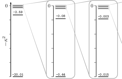
Figure 5: Dimensionless energy eigenvalues $\kappa^{2}$ of the (0,0) band are shown for $\lambda=20$. Accumulation of energy levels as $(-\kappa^{2})\rightarrow 0^{-}$ is obvious and also demonstrated by magnifying the spectrum around the zero energy. The scales on each axis are different.

In fig. 5, we display the dimensionless energy spectrum of the electron in the field of the finite electric dipole for $\lambda=20$, for which $\gamma\approx 5.38$. The accumulation of bound states as $E\rightarrow 0^{-}$ is emphasized by magnifying the spectrum around zero energy, and continues indefinitely.

4 Outlook

We propose an experimentally feasible scenario to observe this geometrical scaling. Our suggestion involves positively and negatively charged quantum dots [33]. By assembling two such dots (representing our fixed charges) onto an insulator matrix one could design a near ideal representation of our model system. This realisation lacks the full rotational symmetry around the axis of the dipole, contrary to our model analysed above, however it only restricts the possible values of the $m$ quantum number to even integers and should not alter the infinite number of bound states and their scaling property. The loosely bound states could be detected by standard photo-detachment spectroscopy [34]. The additional advantage of this scenario would be the possibility of tailoring the dipole moment to a favourable value.

5 Conclusion

We have investigated the energy spectrum of a charged particle’s bound states in the field of a fixed, finite dipole. Using an exact numerical approach, we have confirmed the numerical values of previously known critical dipole moments required to bind the charged particle in different symmetry states. The new result is that for each set of fixed quantum numbers ($n_{\eta}$, $m$) there are an infinite number of bound states, labelled by $n_{\xi}$, for which the consecutive energy eigenvalues are ordered in geometrical scaling. We refer to this scaling as Efimov-like because geometric scaling of the bound state energy levels is a signature of the Efimov effect. We also find an accumulation of states near zero energy, as in the Efimov states. However, our system is not equivalent to Efimov’s original scenario. In the classic Efimov effect, three identical (neutral) bosons interact pair-wise via a short-range potential, with the result that an infinite series of excited three-body energy levels appear only when at least two of the two-body subsystems are at threshold. In our model, we have a long-ranged electrostatic dipolar interaction, and the three particles are distinguishable. Furthermore, the geometric scaling and accumulation of energies, $E\rightarrow 0^{-}$, in our system occurs for any $\lambda\geq\lambda(n_{\eta},m)$. Nevertheless, the common origin for the geometric scaling in both cases is the presence of an inverse square potential in the description of the bound state energy spectrum of the system. We have also suggested a possible experimental scenario in which the results of this paper could be investigated.

- [1] \NameFermi E. Teller E. \REVIEWPhys. Rev.721947399.
- [2] \NameKlahn T. Krebs P. \REVIEWJ. Chem. Phys.1091998531.
- [3] \NameFry P. W., Itskevich I. E., Mowbray D. J., Skolnick M. S., Finley J. J., Barker J. A., O’Reilly E. P., Wilson L. R., Larkin I. A., Maksym P. A., Hopkinson M., Al-Khafaji M., David J. P. R., Cullis A. G., Hill G. Clark J. C. \REVIEWPhys. Rev. Lett.842000733.
- [4] \NameMorse P. M. Stueckelberg E. C. G. \REVIEWPhys. Rev.331929932.
- [5] \NameDesfrançois C., Bouteiller Y., Schermann J. P., Radisic D., Stokes S. T., Bowen K. H., Hammer N. I. Compton R. N. \REVIEWPhys. Rev. Lett.922004083003.
- [6] \NameWallis R. F., Herman R. Milnes H. W. \REVIEWJ. Mol. Spect.4196051.
- [7] \NamePower J. D. \REVIEWPhil. Trans. Roy. Soc. London. A, Math. Phys. Sci.2741973663.
- [8] \NameCrawford O. H. \REVIEWProceedings of the Physical Society911967279.
- [9] \NameTurner J. E., Anderson V. E. Fox K. \REVIEWPhys. Rev.174196881.
- [10] \NameMezei J. Zs. Papp Z. \REVIEWPhys. Rev. A732006030701(R).
- [11] \NamePapp Z., Darai J., Mezei J. Zs., Hlousek Z. T. Hu C-. Y. \REVIEWPhys. Rev. Lett942005143201.
- [12] \NameGarrett W. R. \REVIEWPhys. Rev. A.31971961.
- [13] \NameGarrett W. R. \REVIEWPhys. Rev. A.2219801769.
- [14] \NameKnoop S., Ferlaino F., Mark M., Berninger M., Schobel H., Nägerl H.-C. Grimm R. \REVIEWNat. Phys.52009227.
- [15] \NameFerlaino F., Knoop S., Berninger M., Harm W., D’Incao J. P., Nägerl H.-C. Grimm R. \REVIEWPhys. Rev. Lett.1022009140401.
- [16] \NameTurner J. E. \REVIEWAm. J. Phys.451977758.
- [17] \NameEfimov V. \REVIEWPhys. Lett. B.331970563.
- [18] \NameBraaten E. Hammer H. \REVIEWAnn. Phys.3222007120.
- [19] \NameAmado R. D. Noble J. V. \REVIEWPhys. Lett.35B197125
- [20] \NameChatterjee A. \BookBinding of a charged particle in presence of an electric dipole and a magnetic field Master’s thesis School of Graduate Studies (2008).
- [21] \NameTurner J. Fox K. \REVIEWPhys. Lett.231966547.
- [22] \NameBrown W. B. Roberts R. E. \REVIEWJ. Chem. Phys.4619672006.
- [23] \NameConnolly K. Griffiths D. J. \REVIEWAm. J. Phys.752007524.
- [24] \NameAlhaidari A. D. Bahlouli H. \REVIEWPhys. Rev. Lett.1002008110401.
- [25] \NameEfimov V. \REVIEWNucl. Phys. A.362198145.
- [26] \NameJudd B. R. \BookAngular momentum theory for diatomic molecules (Academic Press Inc., 111 Fifth Avenue, New York 10003) 1975.
- [27] \NameErikson H. A. Hill E. L. \REVIEWPhys. Rev.75194929.
- [28] \NameCoulson C. A. Joseph A. \REVIEWInt. J. Quant. Chem.11967337.
- [29] \NameAbramov D. I. Komarov I. V. \REVIEWTheor. Math. Phys.1319721090.
- [30] \NameRonveaux A. (Editor) \BookHeun’s Differential Equations Oxford Science Publications (Oxford University Press, USA) 1995.
- [31] \NameBates D. R., Ledsham K. Stewart A. L. \REVIEWPhil. Trans. Roy. Soc. London. A, Math. Phys. Sci.2461953215.
- [32] \NameMakarewicz J. \REVIEWJ. Phys. A: Math. Gen.2219894089.
- [33] \NameFindeis F., Baier M., Zrenner A., Bichler M., Abstreiter G., Hohenester U. Molinari E. \REVIEWPhys. Rev. B.632001121309.
- [34] \NameMead R. D., Lykke, K. R., Lineberger, W. C., Marks, J. Brauman, J. I. \REVIEWJ. Chem. Phys.8119844883.