Scheduling Heterogeneous Real-Time Traffic over Fading Wireless Channels

Abstract

We develop a general approach for designing scheduling policies for real-time traffic over wireless channels. We extend prior work, which characterizes a real-time flow by its traffic pattern, delay bound, timely-throughput requirement, and channel reliability, to allow time-varying channels, allow clients to have different deadlines, and allow for the optional employment of rate adaptation. Thus, our model allow the treatment of more realistic fading channels as well as scenarios with mobile nodes, and the usage of more general transmission strategies.

We derive a sufficient condition for a scheduling policy to be feasibility optimal, and thereby establish a class of feasibility optimal policies. We demonstrate the utility of the identified class by deriving a feasibility optimal policy for the scenario with rate adaptation, time-varying channels, and heterogeneous delay bounds. When rate adaptation is not available, we also derive a feasibility optimal policy for time-varying channels. For the scenario where rate adaptation is not available but clients have different delay bounds, we describe a heuristic. Simulation results are also presented which indicate the usefulness of the scheduling policies for more realistic and complex scenarios.

I Introduction

With the wide deployment of Wireless Local Area Networks (WLANs) and advances in multimedia technology, wireless networks are increasingly being used to carry real-time traffic, such as VoIP and video streaming. These applications usually specify throughput requirement while meeting specified delay bounds. We study the problem of designing scheduling policies for such applications.

While there has been much research on scheduling real-time traffic over wireline networks, the results are not directly applicable to wireless networks where channels are unreliable, with qualities that may be time-varying either due to fading or node mobility. Also, individual clients may impose differing delay requirements. These features present new challenges to the scheduling problems.

We consider the scenario where an Access Point (AP) is required to serve real-time traffic for a set of clients. A previous work [10] solves the scheduling problem in a restrictive environment and proposes two feasibility optimal policies. In particular, it assumes a fixed transmission rate, a static channel model, and that all clients in the system require the same delay bound. We extend this model so that it can capture the traffic patterns, delay bounds, timely-throughput bounds, and delivery ratio bounds of clients, for time-varying wireless channels. We address scenarios with and without rate adaptation. We establish a sufficient condition for a scheduling policy to be feasibility optimal. Based on this we describe a class of policies and prove that they are all feasibility optimal.

To demonstrate the utility of the class of policies, we study three particular scenarios of interest. The first scenario employs rate adaptation and treats time-varying channels, as well as allowing different delay bounds for different clients. The other two scenarios treat the case where rate adaptation is not available. One scenario considers time-varying channels, while the other considers the scenario where clients require different delay bounds. For the former two scenarios, we derive computationally tractable scheduling policies and prove that they are feasibility optimal. We also obtain a heuristic for the third scenario.

We have also tested the derived policies using the IEEE 802.11 standard in a simulation environment. The results suggest that the three policies outperform others, including the policies in [10], and a server-centric policy that schedules packets randomly. In particular, since the policies introduced in the previous work fail to provide satisfactory performance in the environments studied here, this suggests that neglecting the facts that the system can apply rate adaptation, that wireless channels are time-varying, and the possibility that clients may require different delay bounds, can result in malperformance of the derived policies.

Section II reviews some of the related work. Section III describes the extension of the model in [10]. Section IV discusses some useful observations for scheduling and reviews policies proposed in [10]. In Section V, we study an extension for time-varying channels. In Section VI, we derive a general class of policies that are feasibility optimal. Based on this class, we obtain scheduling policies in Sections VII and VIII, and a heuristic in Section IX, for different scenarios. In Section X, we discuss implementation issues and simulation results. Section XI concludes the paper.

II Related Work

The problem of providing QoS over unreliable wireless channels has received growing interest in recent years. Tassiulas and Ephremides [18] have considered the problem in a single-hop network by assuming ON/OFF channels and derived a throughput-optimal policy. Though the policy is unaware of packet delay, Neely [15] has shown that average packet delay is constant regardless of the network size. Andrews et al [1] have proposed another policy that aims to improve packet delay. They have proved that their policy is also throughput optimal but offer no theoretical bound on packet delays. Liu, Wang, and Giannakis [14] have used a cross-layer approach to provide differentiated service for a variety of classes of clients. Grilo, Macedo, and Nunes [8] have proposed a resource-allocation algorithm based on the expected transmission time of each packet. Since the expected transmission time may not be an accurate indication of the actual transmission time, their work cannot provide provable delay guarantees. Raghunathan et al [16] and Shakkottai and Srikant [17] have both approached this problem by analytically demonstrating algorithms to minimize the total number of expired packets in the system. Their results, however, cannot provide differentiated service to different clients. Hou, Borkar, and Kumar [9] have studied the problem of providing QoS based on delay bounds and delivery ratio requirements, and proposed two optimal policies under some restrictive assumptions. Their work has been further extended to deal with variable-bit-rate traffic [10]. In this paper, we extend this work to more realistic scenarios, including rate adaptation, time-varying channels and heterogeneous delay bounds among clients. Fattah and Leung [6] and Cao and Li [3] have surveyed other existing scheduling policies for providing QoS.

III System Model

We begin by extending the model proposed in [10], which only considers a static channel condition and fixed delay bounds for all clients, to account for network behavior and application requirements for providing QoS in wireless systems.

Consider a wireless system with $N$ clients, $\{1,2,\dots,N\}$, and one access point (AP). Packets for clients arrive at the AP. Time is slotted with slots $t\in\{0,1,2,\dots\}$. Time slots are further grouped into periods $[kT,(k+1)T)$ with period length $T$. Packets arrive at the AP at the beginning of each period, at time slots $\{0,T,2T,\dots\}$, probabilistically, with no more than one packet per client. We model the packet arrivals as a stationary, irreducible Markov process with finite state. The average probability that packets arrive for subset $S$ of clients is $R(S)$. Packet arrivals can be dependent between clients, and packet arrivals in a period can depend on other periods.

Each client $n$ specifies a delay requirement $\tau_{n}$, with $\tau_{n}\leq T$. If the packet for client $n$ is not delivered by the ${\tau_{n}}^{th}$ time slot of the period, the packet expires and is discarded. This scheme applies naturally to a wide range of server-centric wireless communication technologies, such as IEEE 802.11 Point Coordination Function (PCF), WiMax, and Bluetooth.

We consider an unreliable, heterogeneous, and time-varying channel model. We model the channel condition as a stationary, irreducible Markov process with a finite set of channel states $\mathcal{C}$. The average probability that channel state $c$ occurs is $f_{c}$ and the channel state remains constant within each period. We consider the system both with rate adaptation and without. When rate adaptation is not available, that is, when all packets are transmitted at a fixed rate, the AP can make exactly one transmission in each time slot. Under channel state $c$, the link reliability between the AP and client $n$ is $p_{c,n}$, so that a packet transmitted by the AP for client $n$ is delivered with probability $p_{c,n}$. On the other hand, when the system uses rate adaptation, the channel states describe the maximal rates that can be supported between the AP and clients, which in turn decide the service times for transmissions. Under channel state $c$, it takes $s_{c,n}$ time slots to make an error free transmission to client $n$.

The channel state and the packet arrivals in a period are assumed to be independent of each other. We also assume that the AP has knowledge of channel state, as well as whether a transmission is successful, for example, through ACKs, in which case $p_{c,n}$ is the probability that the AP receives an ACK after making a transmission.

Each client $n$ requires a timely-throughput of at least $q_{n}$ packets per period. Since, on average, there are $\sum_{S:n\in S}R(S)$ packets for client $n$ per period, this timely-throughput bound can also be interpreted as a delivery ratio requirement of $\frac{q_{n}}{\sum_{S:n\in S}R(S)}$.

Definition 1

A set of clients, $\{1,2,\dots,N\}$ is fulfilled under a scheduling policy $\eta$, if for every $\epsilon>0$,

$$Prob\{\frac{d_{n}(t)}{t/T}>q_{n}-\epsilon\mbox{, for every $n$}\}\rightarrow 1\mbox{, as }t\rightarrow\infty,$$

where $d_{n}(t)$ is the number of packets delivered to client $n$ up to time $t$.

IV Scheduling Policies

Since the overall system can be viewed as a controlled Markov chain, we have:

Lemma 1

For any set of clients that can be fulfilled, there exists a stationary randomized policy that fulfills the clients, which uses a probability distribution based only on the channel state, the set of undelivered packets, and the number of time slots remaining in the system (and not any events depending on past periods), according to which it randomly chooses an undelivered packet to transmit, or stays idle.

Since the computational overhead for some complex policies may be too high for real-time applications, we consider the limited set of priority-based policies, which require computation only at the beginning of each period:

Definition 2

A priority-based policy is a scheduling policy which assigns priorities to some of the clients, based on past history and current state of the system, at the beginning of each period. During the period, a packet for a client is transmitted only after all packets for clients with higher priorities have been delivered. Packets for clients which do not receive a priority are never transmitted. A stationary randomized priority-based policy is one which chooses the priority order randomly according to a probability distribution that depends only on the channel state and packet arrivals at the beginning of each period. We denote by $\mathbb{P}$ and $\mathbb{P}_{rand}$ the sets of priority-based policies and stationary randomized priority-based policies.

Definition 3

A set of clients is feasible in the set $\mathbb{P}$ (or $\mathbb{P}_{rand}$) if there exists some scheduling policy in $\mathbb{P}$ (or $\mathbb{P}_{rand}$) that fulfills it.

Similar to Lemma 1, if $[q_{n}]$ is feasible in the set $\mathbb{P}$, it is also feasible in the set $\mathbb{P}_{rand}$.

Definition 4

We call the region in the $N$-space formed by vectors $[q_{n}]$ for which the clients are feasible in $\mathbb{P}$ (or all policies), as the feasible region under $\mathbb{P}$ (or all policies).

Lemma 2

The feasible region under the class of all policies, or $\mathbb{P}$, are both convex sets.

Proof:

Let $[q_{n}]$ and $[q^{\prime}_{n}]$ be two vectors in the feasible region under $\mathbb{P}$, and thus also feasible in $\mathbb{P}_{rand}$. Let $\eta$ and $\eta^{\prime}$ be policies in $\mathbb{P}_{rand}$ that fulfill the two vectors, respectively. Then, the policy in $\mathbb{P}$ that randomly picks one of the two policies, with $\eta$ being chosen with probability $\alpha$, at the beginning of each period, fulfills the vector $[\alpha q_{n}+(1-\alpha)q^{\prime}_{n}]$. Further, since $q_{n}$ and $q^{\prime}_{n}$ are both larger than 0 for each $n$, $\alpha q_{n}+(1-\alpha)q^{\prime}_{n}>0$ for all $n$. Thus, the vector $[\alpha q_{n}+(1-\alpha)q^{\prime}_{n}]$ also falls in the feasible region under $\mathbb{P}$. A similar proof holds for the class of all policies. ∎

Note that if $[q_{n}]$ is feasible in $\mathbb{P}$, then so is $[q^{\prime}_{n}]$, where $0<q_{n}^{\prime}\leq q_{n}$.

Definition 5

$[q_{n}]$ is strictly feasible in $\mathbb{P}$ (or the class of all policies) if there exists some $\alpha\in(0,1)$ such that $[q_{n}/\alpha]$ is feasible in $\mathbb{P}$ (or the class of all policies).

Definition 6

A scheduling policy $\eta$ is feasibility optimal among $\mathbb{P}$ (or the class of all policies) if it fulfills every set of clients that is strictly feasible in $\mathbb{P}$ (or the class of all policies).

In the rest of the paper, unless otherwise specified, the default is the set of all policies.

IV-A The Static Channel Case

In previous work [10], the problem of admission control and feasibility optimal scheduling has been addressed for the case where the channel state is static, and all clients require the same delay bounds, i.e. $|\mathcal{C}|=1$ and $\tau_{n}\equiv\tau$. In the special case, we will use $p_{n}$ instead of $p_{c,n}$ since the channel state is static, and $\tau$ instead of $\tau_{n}$.

Two largest debt first scheduling polices were proved to be feasibility optimal, where the AP, based on the past history, calculates a debt for each client. In each period, the AP sorts all clients according to their debts, and schedules a packet for client $n$ only after all packets for clients with larger debts have been delivered. The first policy, the largest time-based debt first policy, uses the time-based debt for client $n$ at time slot $t$, defined as $\frac{t}{T}w_{n}$ minus the number of time slots that the AP has spent on transmitting packets for client $n$ up to time slot $t$. The other policy, the largest weighted-delivery debt first policy, uses the weighted-delivery debt for client $n$ at time slot $t$, defined as $\frac{\frac{t}{T}q_{n}-d_{n}(t)}{p_{n}}$, where $d_{n}(t)$ is the number of delivered packets for client $n$ up to time slot $t$.

As for admission control, the following lemma was proved in [10]:

Lemma 3

A set of clients is fulfilled if and only if the long-term average number of time slots that the AP spends on transmitting packets for client $n$ per period is at least $w_{n}=\frac{q_{n}}{p_{n}}$ for each $n$.

Further, since expired packets are dropped, the number of packets in the system is bounded. Thus, there may be some time slots where the AP may have delivered all packets in the system, and is therefore forced to stay idle. For any subset $S$ of $\{1,2,\dots,N\}$, define $I_{S}$ to be the minimum number of time slots that the AP is idle in a period for any scheduling policy, given that the AP can only transmit packets for the subset $S$ of clients. A necessary and sufficient condition for strict feasibility is proved:

Theorem 1

A set of clients is strictly feasible if and only if $\sum_{n\in S}w_{n}<T-E[I_{S}]$, for all $S\subseteq\{1,2\dots,N\}$.

V Time-Varying Channels

We now discuss how to extend the aforementioned policies to provide QoS for time-varying channels. One intuitive approach is to decouple the channel states. The AP assigns a timely-throughput requirement $q_{c,n}$ for each channel state $c$ and client $n$, with $\sum_{c\in\mathcal{C}}f_{c}q_{c,n}\geq q_{n}$. Also, for each channel state $c$, the assigned throughput requirements must be strictly feasible under that channel state, that is, $\sum_{n\in S}\frac{q_{c,n}}{p_{c,n}}<T-E[I_{c,S}]$ for all $S\subseteq\{1,2,\dots,N\}$ , where $I_{c,S}$ is the minimal number of time slots that the AP is forced to stay idle in a period under channel state $c$ for any scheduling policy, given that the AP only transmits packets for the subset $S$ of clients. More formally, we therefore seek a matrix $Q=[q_{c,n}]$ that solves the following linear programming problem:

$$\mbox{Max }\mbox{$\sum_{n=1}^{N}\sum_{c\in\mathcal{C}}$}f_{c}q_{c,n}$$

s.t. $$\mbox{$\sum_{c\in\mathcal{C}}$}f_{c}q_{c,n}\geq q_{n},\forall n$$

$$\mbox{$\sum_{n\in S}$}\frac{q_{c,n}}{p_{c,n}}<T-E[I_{c,S}],\forall c,\forall S\subseteq\{1,2,\cdots,N\}.$$

After obtaining the matrix $Q$, we can modify the two largest debt first policies to deal with time-varying channel conditions. Let $s_{c}(t)$ be the number of time slots up to time slot $t$ that the channel state has been $c$, and assume that the channel state at time slot $t$ is $c$. In the largest time-based debt first policy, we define the time-based debt for client $n$ under channel state $c$ as $\frac{s_{c}(t)}{T}\frac{q_{c,n}}{p_{c,n}}$ minus the number of time slots that the AP has spent on transmitting packets for client $n$ under channel state $c$ up to time slot $t$. In the largest weighted-delivery debt first policy, we define the weighted-delivery debt for client $n$ under channel state $c$ as $\frac{\frac{s_{c}(t)}{T}q_{c,n}-d_{c,n}(t)}{p_{c,n}}$, where $d_{c,n}(t)$ is the number of delivered packets for client $n$ under channel state $c$. Obviously, these two modified largest debt first policies are feasibility optimal.

While this extension offers feasibility optimality, the above linear program involves exponentially many constraints. Further, it also requires the knowledge of the distribution $[p_{c,n}]$ of channel states. In many scenarios, such as those with mobile nodes, this knowledge may not be available. This motivates us, in the following sections, to describe a more general class of feasibility optimality policies, and derive an on-line scheduling policy that is feasibility optimal for the time-varying channel conditions.

VI A Sufficient Condition for Feasibility Optimality

We now describe a more general class of policies that is feasibility optimal. We start by extending the concept of “debt”.

Definition 7

A variable $r_{n}(k)$, whose value is determined by the past history of the client $n$ up to the $k^{th}$ period, or time slot $kT$, is called a pseudo-debt if:

1. $r_{n}(0)=0$, for all $n$.

2. At the beginning of each period, $r_{n}(k)$ increases by a constant strictly positive number $z_{n}=z_{n}(q_{n})$, which is an increasing linear function of $q_{n}$.

3. $r_{n}(k+1)=r_{n}(k)+z_{n}(q_{n})-\mu_{n}(k)$, where $\mu_{n}(k)$ is a non-negative and bounded random variable whose value is determined by the behavior of client $n$. Further, $\mu_{n}(k)=0$ if the AP does not transmit any packet for client $n$.

4. The set of clients is fulfilled if and only if $Prob\{\frac{r_{n}(k)}{k}<\varepsilon\}\rightarrow 1$, as $k\rightarrow\infty$, for all $n$ and all $\varepsilon>0$.

In the following example, we illustrate that both the time-based debt and the weighted-delivery debt are pseudo-debts under a static channel model.

Example 1

At the beginning of each period, the time-based debt $r^{(1)}_{n}(k)$ increases by $w_{n}=\frac{q_{n}}{p_{n}}$, and decreases by the number of time slots that the AP has transmitted packets for client $n$ during the period. Lemma 3 shows that condition (4) is satisfied.

Similarly, $r^{(2)}_{n}(k)$, the weighted-delivery debt is also a special case. It increases by $\frac{q_{n}}{p_{n}}$ at the beginning of each period, and decreases by $\frac{1}{p_{n}}$ if a packet is delivered for client $n$ during that period, and 0 otherwise. It satisfies condition (4) by definition. $\Box$

We can also define the feasible region for debt in $\mathbb{P}$ (or in the set of all policies) as the set of $[z_{n}]$ such that the corresponding $[q_{n}]$ is feasible in $\mathbb{P}$ (or in the set of all policies). Since $z_{n}$ is a linear function of $q_{n}$ and the feasible region for $[q_{n}]$ is a convex set (Lemma 2), the feasible region for $[z_{n}]$ is also a convex set.

Using the concept of pseudo-debt, we prove a sufficient condition for feasibility optimality. The proof resembles one used by Neely [15], though in a different context, and is based on:

Theorem 2 (Lyapunov Drift Theorem)

Let $L(t)$ be a non-negative Lyapunov function. Suppose there exists some constant $B>0$ and non-negative function $f(t)$ adapted to the past history of the system such that:

$$E\{L(t+1)-L(t)|\mbox{history up to time $t$}\}\leq B-\epsilon f(t),$$

for all $t$, then: $\limsup_{t\rightarrow\infty}\frac{1}{t}\sum_{i=0}^{t}E\{f(i)\}\leq B/\epsilon.$ $\Box$

Theorem 3

Let $r_{n}(k)$ be a pseudo-debt.

1. A policy that maximizes the payoff function

   $$\sum_{n=1}^{N}E\{r_{n}(k)^{+}\mu_{n}(k)|c_{k},S_{k},[r_{m}(k)]\}$$ (1)

   at the beginning of each period is feasibility optimal, where $c_{k}$ denotes the channel state in the $k^{th}$ period, and $S_{k}$ is the subset of clients whose packets arrive at the AP at the beginning of the $k^{th}$ period.

2. A priority-based policy that maximizes (1) over all policies in $\mathbb{P}$ is feasibility optimal in $\mathbb{P}$.

Proof:

We present the proof for $\mathbb{P}$ only. A similar proof works for the class of all policies too. Define $L(k)=\frac{1}{2}\sum_{n=1}^{N}r_{n}(k)^{2}.$ Since $r_{n}(k+1)=r_{n}(k)+z_{n}-\mu_{n}(k)$,

$$\Delta(L(k)):=E\{L(k+1)-L(k)|[r_{m}(k)]\}$$

$$= E\{\frac{1}{2}\sum_{n=1}^{N}r_{n}(k+1)^{2}-\frac{1}{2}\sum_{n=1}^{N}r_{n}(k)^{2}|[r_{m}(k)]\}$$

$$= E\{\sum_{n=1}^{N}r_{n}(k)[z_{n}-\mu_{n}(k)]+\frac{1}{2}\sum_{n=1}^{N}[z_{n}-\mu_{n}(k)]^{2}|[r_{m}(k)]\}.$$

Define $B(k):=E\{\frac{1}{2}\sum_{n=1}^{N}[z_{n}-\mu_{n}(k)]^{2}|[r_{m}(k)]\}$. Then $B(k)\leq B$, for all $k$, for some $B$. Hence for any policy in $\mathbb{P}$:

$$\Delta(L(k))\leq E\{\sum_{n=1}^{N}r_{n}(k)[z_{n}-\mu_{n}(k)]|[r_{m}(k)]\}+B.$$ (2)

Suppose $[q_{n}]$ is strictly feasible in $\mathbb{P}$. The vector $[z_{n}]$ is thus an interior point of the feasible region (for debt) under $\mathbb{P}$, and there therefore exists some $\alpha\in(0,1)$ such that $[z_{n}/\alpha]$ is also in the feasible region under $\mathbb{P}$. Let $z_{min}=\min\{z_{1},z_{2},\dots,z_{N}\}$. The $N$-dimensional vector $[z_{min}]$ whose elements are all $z_{min}$, falls in the feasible region under $\mathbb{P}$. Since the feasible region under $\mathbb{P}$ is a convex set, the vector $\alpha[z_{n}/\alpha]+(1-\alpha)[z_{min}]=[z_{n}+(1-\alpha)z_{min}]$ is also in the feasible region under $\mathbb{P}$.

By Lemma 1, there exists a stationary randomized policy $\eta^{\prime}$ in $\mathbb{P}$ that fulfills the set of clients with timely-throughput bounds for the vector $[z_{n}+(1-\alpha)z_{min}]$. Let $\mu^{\prime}_{n}(k)$ be the decrease in the pseudo-debt for client $n$ under $\eta^{\prime}$ during the period. Then, we have:

$$E\{\mu^{\prime}_{n}(k)|[r_{m}(k)]\} =E\{E\{\mu^{\prime}_{n}(k)|c_{k},S_{k},[r_{m}(k)]\}\}$$

$$\geq z_{n}+(1-\alpha)z_{min}.$$

Above, the outer expectation in the RHS is taken over channel states and the vectors of packet arrivals.

Let $\eta$ be a policy that maximizes the payoff function (1), for all $k$, among all policies in $\mathbb{P}$. Then defining $\mu_{n}(k)$ and $r_{n}(k)$ as the decrease resulting from policy $\eta$ and the pseudo-debt, we have:

$$\mbox{$\sum_{n=1}^{N}$}E\{r_{n}(k)^{+}\mu_{n}(k)|c_{k},S_{k},[r_{m}(k)]\}$$

$$\geq \mbox{$\sum_{n=1}^{N}$}E\{r_{n}(k)^{+}\mu^{\prime}_{n}(k)|c_{k},S_{k},[r_{m}(k)]\}.$$

We can assume without loss of generality that the policy does not work on any client $n$ with $r_{n}(k)\leq 0$, that is, $\mu_{n}(k)=0$ if $r_{n}(k)\leq 0$. From (2), we obtain:

$$\Delta(L(k)) \leq E\{\mbox{$\sum_{n=1}^{N}$}r_{n}(k)^{+}[z_{n}-\mu_{n}(k)]|[r_{m}(k)]\}+B$$

$$\leq E\{\mbox{$\sum_{n=1}^{N}$}r_{n}(k)^{+}[z_{n}-\mu^{\prime}_{n}(k)]|[r_{m}(k)]\}+B$$

$$\leq-\mbox{$\sum_{n=1}^{N}$}r_{n}(k)^{+}(1-\alpha)z_{min}+B.$$

Let $\epsilon:=(1-\alpha)z_{min}$. By Theorem 2,

$$\mbox{$\limsup_{k\rightarrow\infty}\frac{1}{k}\sum_{i=0}^{k}E\{\sum_{n=1}^{N}r_{n}(k)^{+}\}\leq B/\epsilon$}.$$ (3)

Finally, since $z_{n}$ is a constant and $\mu_{n}(k)$ is a bounded function, $|r_{n}(k+1)-r_{n}(k)|$ is bounded, which implies that $|\sum_{n=1}^{N}r_{n}(k+1)^{+}-\sum_{n=1}^{N}r_{n}(k)^{+}|$ is also bounded for all $k$. Thus, (3) implies that $\frac{1}{k}E\{\sum_{n=1}^{N}r_{n}(k)^{+}\}\rightarrow 0$ as $k\rightarrow\infty$, as shown in Lemma 4 below. This shows that $\frac{{r_{n}(k)}^{+}}{k}$ converges to 0 in probability for all $n$. Hence, $\eta$ is feasibility optimal in $\mathbb{P}$. ∎

Lemma 4

Let $f(t)$ be a non-negative function such that $|f(t+1)-f(t)|\leq M$, for some $M>0$, for all $t$. If $\limsup_{t\rightarrow\infty}\frac{1}{t}\sum_{i=0}^{t}f(i)\leq B/\epsilon,$ then $\lim_{t\rightarrow\infty}\frac{1}{t}f(t)=0.$

Proof:

We prove by contradiction. Suppose $\limsup_{t\rightarrow\infty}\frac{1}{t}f(t)>\delta$, for some $\delta>0$. Thus, $f(t)>t\delta$ infinitely often. Suppose $f(t)>t\delta$ for some $t$. Since $|f(t)-f(t-1)|<M$, we have $f(t-1)>t\delta-M$. Similarly, $f(t-2)>t\delta-2M,$ $f(t-3)>t\delta-3M,\dots,f(t-\lfloor t\delta/M\rfloor)>t\delta-\lfloor t\delta/M\rfloor M\geq 0$. Summing over these terms gives: $\sum_{i=t-\lfloor t\delta/M\rfloor}^{t}f(i)>\frac{t\delta\lfloor t\delta/M\rfloor}{2},$ and thus, $\sum_{i=0}^{t}\frac{1}{t}f(i)>\frac{\delta\lfloor t\delta/M\rfloor}{2}.$ Since $f(t)>t\delta$ infinitely often, $\limsup_{t\rightarrow\infty}\sum_{i=0}^{t}\frac{1}{t}f(i)=\infty,$ which is a contradiction. ∎

Theorem 3 suggests a more general procedure to design feasibility optimal scheduling policies. To design a scheduling policy in a particular scenario, we need to choose an appropriate pseudo-debt and obtain a policy to maximize the payoff function. Maximizing the payoff function is, however, in general, difficult. Nevertheless, in some special cases, evaluating the payoff function gives us simple feasibility optimal policies, or, at least, some insights into designing a reasonable heuristic, as long as we choose the correct pseudo-debt. In the following sections, we demonstrate the utility of this approach.

VII Scheduling Policy with Rate Adaptation

We now propose a feasibility optimal scheduling policy when rate adaptation is employed. Channel qualities can be time-varying and clients may have different deadlines.

To derive the scheduling policy, we define the delivery debt $r_{n}^{(3)}(k):=q_{n}k-d_{n}(kT),$ where $d_{n}(t)$ is the number of delivered packets for client $n$ up to time slot $t$. Thus, $z_{n}:=q_{n}$, while $\mu_{n}(k)=1$ if a packet for client $n$ is delivered in the period, and $\mu_{n}(k)=0$ otherwise.

Suppose at the beginning of period $k$, the delivery debt vector is $[r_{n}^{(3)}(k)]$, the channel state is $c$, and the set of arrived packets is $S$. The transmission time for client $n$ is $s_{c,n}$ time slots, and client $n$ stipulates a delay bound of $\tau_{n}$. Since transmissions are assumed to be error-free when rate adaptation is applied, the scheduling policy consists of finding an ordered subset $S^{\prime}=\{m_{1},m_{2},\dots,m_{N^{\prime}}\}$ of $S$ such that $\sum_{n=1}^{l}s_{c,n}\leq\tau_{l}$, for all $1\leq l\leq m_{N^{\prime}}$. That is, when clients are scheduled according to the ordering, no packets for clients in $S^{\prime}$ would miss their respective delay bounds. By Theorem 3, a policy using an ordered set $S^{\prime}$ that maximizes $\sum_{n\in S^{\prime}}r_{n}^{(3)}(k)$ with the above constraint is feasibility optimal. This is a variation of the knapsack problem. When $S^{\prime}$ is selected, reordering clients in $S^{\prime}$ in an earliest-deadline-first fashion also allows all packets to meet their respective delay bounds. Based on this observation, we derive the feasibility optimal scheduling algorithm, the Modified Knapsack Algorithm. Let $M[n,t]$ be the maximum debt a policy can collect if only clients $1$ through $n$ can be scheduled and all transmissions need to complete before time slot $t$. Thus, $\max_{S^{\prime}}\sum_{n\in S^{\prime}}r_{n}^{(3)}(k)=M[N,T]$. Also, iteratively:

$$M[n,t]=\left\{\begin{array}[]{lr}M[n,t-1]&\mbox{if }t>\tau_{n},\\ \max\{M[n-1,t],\\ r_{n}^{(3)}(k)+M[n-1,t-s_{c,n}]\}&\mbox{otherwise,}\end{array}\right.$$

where $M[n-1,t]$ is the maximum debt can be collected when client $n$ is not scheduled, and $r_{n}^{(3)}(k)+M[n-1,t-s_{c,n}]$ is that when client $n$ is scheduled. The complexity of this algorithm is $O(N\tau)$, and it is thus reasonably efficient.

Algorithm 1 Modified Knapsack Policy

1:  for $n=1$ to $N$ do

2:     $r_{n}^{(3)}(k)=q_{n}k-d_{n}(kT)$

3:  Sort clients such that $\tau_{1}\leq\tau_{2}\leq\dots\leq\tau_{N}$

4:  $S^{\prime}[0,0]=\phi$

5:  $M[0,0]=0$

6:  for $n=1$ to $N$ do

7:     for $t=1$ to $T$ do

8:        if $t>\tau_{n}$ then

9:           $M[n,t]=M[n,t-1]$

10:           $S^{\prime}[n,t]=S^{\prime}[n,t-1]$

11:        else if client $n$ has a packet AND$r_{n}^{(3)}(k)+M[n-1,t-s_{c,n}]>M[n-1,t]$ then

12:           $M[n,t]=r_{n}^{(3)}(k)+M[n-1,t-s_{c,n}]$

13:           $S^{\prime}[n,t]=S^{\prime}[n-1,t-s_{c,n}]+\{n\}$

14:        else

15:           $M[n,t]=M[n-1,t]$

16:           $S^{\prime}[n,t]=S^{\prime}[n-1,t]$

17:  schedule according to $S^{\prime}[N,T]$

VIII Computationally Tractable Scheduling for Time-Varying Channels

We now consider the case when rate adaptation is not available, and propose a scheduling policy for time-varying channels and homogeneous delay bounds. We show that the policy is feasibility optimal among all priority-based policies. We use the delivery debt, $r_{n}^{(3)}(k)$, of Section VII.

Suppose at the beginning of a period, the delivery debt vector is $[r_{n}^{(3)}(k)]$, the channel state is $c$, and the set of arrived packets is $S$. We wish to find the priority ordering that maximizes the payoff function $\mu_{tot}(k)=\sum_{n=1}^{N}r_{n}^{(3)}(k)^{+}E\{\mu_{n}(k)\}$, where in the expectation we suppose that the channel state $c$ and the set of arrival packets $S$ are both fixed. Obviously, transmitting a packet from a client $n$ with $r_{n}^{(3)}(k)\leq 0$ will not increase the value of $\mu_{tot}(k)$. Thus, we do not give priorities to clients with non-positive delivery debts. For ease of the remaining discussion, we further assume $r_{n}^{(3)}(k)>0$ for all $n$.

Consider two orderings, $A$ and $B$: In $A$, the priority order is $\{1,2,\dots,N\}$, while, in $B$, the priority order is $\{1,2,\dots,m-1,m+1,m,m+2,m+3,\dots,N\}$. Let the values of the payoff functions be $\mu_{tot}^{A}$ and $\mu_{tot}^{B}$. Since clients $1$ through $m-1$ have the same priorities in both orderings and their priorities are higher than the remaining clients, the values of $E\{\mu_{n}(k)\},$ $1\leq n\leq m-1$ are the same for both orderings. On the other hand, clients $m+2$ through $N$ also have the same priorities in both orderings and they can be scheduled only after the packets for clients $1$ through $m+1$ are delivered. The probabilities of packet deliveries for these clients are the same under the two orderings. Thus, to compare the two orderings, one only needs to evaluate the probabilities of packet delivery for client $m$ and $m+1$. We further notice that the probabilities that packets for both clients $m$ and $m+1$ are delivered are also the same for both orderings. With $e_{n}$ the event that the packet for client $n$ is delivered,

$$\mu_{tot}^{A}-\mu_{tot}^{B}= r_{m}^{(3)}(k)Prob\{e_{m}\backslash e_{m+1}|\mbox{ordering A}\}$$

$$-r_{m+1}^{(3)}(k)Prob\{e_{m+1}\backslash e_{m}|\mbox{ordering B}\}.$$

Suppose that there are $\tau^{\prime}$ time slots left when all packets from client $1$ through $m-1$ have been delivered. The probability distribution of $\tau^{\prime}$ is the same under both orderings. Since the channel reliability is $p_{c,n}$,

$$\mu_{tot}^{A}-\mu_{tot}^{B}$$

$$= r_{m}^{(3)}(k)E\{\sum_{t=1}^{\tau^{\prime}}p_{c,m}(1-p_{c,m})^{t-1}(1-p_{c,m+1})^{\tau^{\prime}-t}\}$$

$$-r_{m+1}^{(3)}(k)E\{\sum_{t=1}^{\tau^{\prime}}p_{c,m+1}(1-p_{c,m+1})^{t-1}(1-p_{c,m})^{\tau^{\prime}-t}\}$$

$$= [r_{m}^{(3)}(k)p_{c,m}-r_{m+1}^{(3)}(k)p_{c,m+1}]$$

$$\times\mbox{$E\{\sum_{t=0}^{\tau^{\prime}-1}(1-p_{c,m})^{t}(1-p_{c,m+1})^{\tau^{\prime}-t-1}\}.$}$$

Thus, $\mu_{tot}^{A}\geq\mu_{tot}^{B}$ if $r_{m}^{(3)}(k)p_{c,m}\geq r_{m+1}^{(3)}(k)p_{c,m+1}$. This leads us to obtain the Joint Debt-Channel Policy. The computation time is only $O(N\log N)$.

Algorithm 2 Joint Debt-Channel Policy

1:  for $n=1$ to $N$ do

2:     $r_{n}^{(3)}(k)=q_{n}k-d_{n}(kT)$, for all $n$

3:  Sort clients with a packet arrival such that $r_{1}^{(3)}(k)p_{c,1}\geq r_{2}^{(3)}(k)p_{c,2}\geq\dots\geq r_{N_{0}}^{(3)}(k)p_{c,N_{0}}>0\geq r_{N_{0}+1}^{(3)}(k)p_{c,N_{0}+1}\geq\dots$

4:  Transmit packets for clients $1$ through $N_{0}$ by the ordering

Theorem 4

The joint debt-channel policy is feasibility optimal among all priority-based policies.

Proof:

Let $\eta$ be the joint debt-channel policy and $\eta^{\prime}$ any priority-based policy. Suppose the priorities assigned by the policies are $\eta_{1},\eta_{2},\dots,\eta_{m}$, and $\eta^{\prime}_{1},\eta^{\prime}_{2},\dots,\eta^{\prime}_{m^{\prime}}$. We modify $\eta^{\prime}$ as follows:

1. Delete any element in $\eta^{\prime}_{1}\sim\eta^{\prime}_{m^{\prime}}$ with $r^{(3)}_{\eta^{\prime}_{n}}(k)\leq 0$.

2. For any client $n$ with $r^{(3)}_{n}(k)>0$ that is not in $\eta^{\prime}_{1}\sim\eta^{\prime}_{m^{\prime}}$, append it at the end of the ordering.

3. If $\eta^{\prime}_{1}\sim\eta^{\prime}_{m^{\prime}}$ is still different from $\eta_{1}\sim\eta_{m}$, there exists some $n$ such that $r_{\eta^{\prime}_{n}}^{(3)}(k)p_{c,{\eta^{\prime}_{n}}}<r_{\eta^{\prime}_{n+1}}^{(3)}(k)p_{c,{\eta^{\prime}_{n+1}}}$. Swap $\eta^{\prime}_{n}$ and $\eta^{\prime}_{n+1}$.

4. Repeat Step 3 until the two orderings are the same.

Steps 1 and 2 will not decrease the value of the payoff function. As derived above, Step 3 does not decrease the value of the payoff function, either. Thus, $\eta$ maximizes the payoff function and is feasibility optimal in $\mathbb{P}$. ∎

IX A Heuristic for Heterogeneous Delay Bounds

We now describe a heuristic for packet scheduling, for the case where each channel state is static and transmission rate is fixed, but clients require different delay bounds. We use $p_{n}$ to represent channel reliability.

We will use the time-based debt, $r_{n}^{(1)}(k)$, as discussed in Example 1. The payoff function is $E\{\sum_{n=1}^{N}r^{(1)}_{n}(k)^{+}\mu_{n}(k)\}$.

Suppose, without loss of generality, that at the beginning of a period, packets for clients $\{1,2,\dots,N_{0}\}$ arrive. We further assume that $\tau_{1}\leq\tau_{2}\leq\dots\leq\tau_{N_{0}}$. Let $\gamma_{n}$ be the number of transmissions the AP needs to make for client $n$ for success. While $\gamma_{n}$ is a random variable that cannot be foretold, we examine how to maximize $\sum_{n=1}^{N_{0}}r_{n}^{(1)}(k)^{+}\mu_{n}(k)$ if we knew $\gamma_{n}$.

We solve this by proceeding backwards in time. During time slots $[\tau_{N_{0}-1}+1,\tau_{N_{0}}]$, all packets except the one for client $N_{0}$ have expired, and we can only make transmissions for client $N_{0}$ during these time slots. Thus, it does not make sense to schedule client $N_{0}$ for more than $\gamma^{N_{0}-1}_{N_{0}}:=\gamma_{N_{0}}-(\tau_{N_{0}}-\tau_{N_{0}-1})$ transmissions before time slot $\tau_{N_{0}-1}$. Next, in the time slots between $[\tau_{N_{0}-2}+1,\tau_{N_{0}-1}]$, only clients $N_{0}-1$ and $N_{0}$ can be scheduled. An obvious choice is to schedule the client with larger debt first, with the restriction that it is not scheduled for more than $\gamma^{N_{0}-1}_{n}$ time slots, and to then schedule the other client. (For simplicity, we let $\gamma^{N_{0}-1}_{N_{0}-1}:=\gamma_{N_{0}-1}$.) We can further obtain the remaining transmissions allowed for client $n$ before time slot $\tau_{N_{0}-2}$, which we call $\gamma^{N_{0}-2}_{n}$, as $\gamma^{N_{0}-1}_{n}$ minus the number of transmissions scheduled for client $n$ during time slots $[\tau_{N_{0}-2}+1,\tau_{N_{0}-1}]$. Transmissions of the remaining time slots are scheduled similarly.

While it is impossible to know the exact value of $\gamma_{n}$ in advance, we can estimate it. One estimate is its expected value, $\frac{1}{p_{n}}$. However, this estimate does not consider the timely-throughput requirements. If a client has significantly larger debt than others, a reasonably good policy would allocate enough time slots so that the probability of packet delivery for the client in this period is at least its delivery ratio bound, $\frac{q_{n}}{\sum_{n\in S}R(S)}$, given that a packet for client $n$ arrived. So we estimate $\gamma_{n}$ by the number of transmissions that we need to allocate for client $n$ so that it can achieve its delivery ratio bound. Since the channel reliability for client $n$ is $p_{n}$, this estimate $\gamma_{n}$ is $\lceil\log_{1-p_{n}}(1-\frac{q_{n}}{\sum_{n\in S}R(S)})\rceil$. We thus derive the Adaptive-Allocation Policy shown in Algorithm 3.

As a final remark, note that in all the three policies discussed in this paper, we do not schedule transmissions for clients with non-positive debts. This restriction improves the performance for clients with non-real time traffic. In practice, it is possible that clients with real-time traffic and clients with non-real time traffic coexist. Thus, it is important not to allocate too much of the resource to real-time clients and starve those with non-real time traffic.

Algorithm 3 Adaptive-Allocation Policy

1:  for $n=1$ to $N$ do

2:     $r_{n}^{(1)}(k)=$ time-based debt

3:     $\gamma_{n}=\lceil\log_{1-p_{n}}(1-\frac{q_{n}}{\sum_{n\in S}R(S)})\rceil$

4:  Sort clients so that packets for clients $1\sim N_{0}$ arrive and $r_{1}^{(1)}(k)\geq r_{2}^{(1)}(k)\geq\dots\geq r_{N_{0}}^{(1)}(k)$

5:  $alloc\leftarrow n\times 1-$vector

6:  for $t=T$ to $1$ do

7:     $n\leftarrow 1$

8:     while ($\tau_{n}>t$ or $\gamma_{n}\leq 0$) and $n\leq N_{0}$ do

9:        $n\leftarrow n+1$

10:     if $r_{n}^{(1)}(k)>0$ then

11:        $alloc[t]\leftarrow n$

12:     else

13:        $alloc[t]\leftarrow N_{0}+1$

14:     if $n\leq N_{0}$ then

15:        $\gamma_{n}\leftarrow\gamma_{n}-1$

16:  for each time slot $t$ do

17:     if $alloc[t]\leq N_{0}$ and the packet for client $alloc[t]$ has not been delivered then

18:        transmit the packet for client $alloc[t]$

19:     else

20:        transmit the packet with the largest positive time-based debt

X Simulation Results

We have implemented the scheduling policies discussed in previous sections by using the IEEE 802.11 PCF standard in the ns-2 simulator. We present the simulation results for the scenario with time-varying channels, and with clients requiring different delay bounds. In each scenario, we compare our policies against the two largest debt first policies of [10], and a policy that assigns priorities to clients randomly, random. IEEE 802.11e, an enhancement to 802.11 for QoS, allows clients with real-time traffic to use smaller contention window and inter frame space to obtain priorities over clients with non-real time traffic. However, clients with real-time traffic have to compete with each other in a random access manner with equal channel access probabilities, without any QoS based preference or discrimination. Further, the inter frame space and contention window size are smaller in PCF than in 802.11e. Thus, the random policy can be viewed as an improved version of 802.11e. Similar to the previous work, we conduct two sets of simulations for each scenario, one with clients carrying VoIP traffic, and one with clients carrying video streaming traffic. The major difference between the two settings lies in their traffic patterns. Many VoIP codecs generate packets periodically. Thus, future packet arrivals can be easily predicted and may be dependent among different clients. For example, if two clients generate packets at the same rate, then either all or none of their packets arrive simultaneously. On the other hand, video streaming technology, such as MPEG, may generate traffic with variable-bit-rate (VBR). Thus, packets arrive at the AP probabilistically, with probability depending on the context of the current frame, and arrivals are independent among different clients.

For the VoIP traffic, we follow the standards of the ITU-T G.729.1 [12] and G.711 [11] codecs. Both codecs generate traffic periodically. G.729.1 generates traffic with bit rates 8 – 32 kbits/s, while G.711 generates traffic at a higher rate of 64 kbits/s. We assume the period length, $T$, is 20 ms, and the payload size of a packet is 160 Bytes. The codecs generate one packet every several periods; with the duration between packet arrivals depending on the bit rate used.

We use MPEG for the video streaming setting. MPEG VBR traffic is usually modeled as a Markov chain consisting of three activity states [13][5]. Each state generates traffic probabilistically at different mean rates, with the state being determined by the current frame of the video. The statistical mean rates in each state are those obtained in an experimental study [5]. We use them in setting the traffic patterns of MPEG traffic. We assume the period length to be 6 ms and the payload size of a packet to be 1500 Bytes. Table I shows the statistical results of the experimental study [5], where we also present them in terms of the packet arrival probability of our setting. In Table I, “Data rate” is measured in bits/GoP, where 1 GoP= 240 ms.

TABLE I: MPEG Traffic Pattern

Activity	Great	High	Regular
Data rate	501597	392237	366587
Arrival probability	1	0.8	0.75

We simulate 20 runs for each setting, each run lasting one minute in simulated time. All results shown are averaged over the 20 runs. A natural performance metric for a client is the delivery debt, $r_{n}^{(3)}(k)$. The performance of the system is measured by the sum of the positive delivery debts of the clients, that is, $\sum_{n=1}^{N}r_{n}^{(3)}(k)^{+}$, the total delivery debt. In addition to evaluating how well the tested policies serve clients with real-time traffic, we also wish to know whether the policies starve those with non-real time traffic. Hence we add a client with saturated non-real time traffic in all simulations. Packets for the non-real time client are scheduled in all time slots that are left idle otherwise. We measure the throughput of the client with non-real time traffic by the average number of packets delivered.

X-A Rate Adaptation

We present the simulation results under the scenario where rate adaptation is applied, channels are time-varying, and clients may require different delay bounds.

We first show the results for VoIP traffic. We use IEEE 802.11b as the MAC protocol, which can provide a maximum data rate of 11 Mb/s. We assume that the channel capacity of each client alternates between 11 Mb/s and 5.5 Mb/s. Simulation results suggest that the times needed for a transmission, including all MAC overheads such as the time for waiting an ACK, are around 480 $\mu$s and 610 $\mu$s for the two transmission rates, respectively. Ideally, the length of a time slot should be a common divisor of the transmission times needed under the two used data rates. We approximate this value by 160 $\mu$s. Thus, transmitting a packet requires 3 time slots when using 11 Mb/s and 4 time slots when using 5.5 Mb/s. Further, a period consists of 125 time slots.

There are two groups of clients, $A$ and $B$. Clients in group $A$ generate one packet every three periods, or at rate 21.3 kbits/s, and require 90$\%$ of each of the clients’ packets to be delivered, or a timely-throughput requirement of 19.2 kbits/s. Clients in group $B$ generate one packet every two periods at rate 32 kbits/s, and require 70$\%$ of each of the clients’ packets to be delivered, corresponding to a timely-throughput requirement of 22.4 kbits/s. The two groups can be further divided into subgroups, $A_{1}$, $A_{2}$, $A_{3}$, $B_{1}$, and $B_{2}$, each with 22 clients. Clients in subgroup $A_{i}$ generate packets at periods $[i,i+3,i+6,\dots]$, and clients in subgroup $B_{i}$ generate packets at periods $[i,i+2,i+4,\dots]$. Finally, clients in group $A$ require a delay bound equal to the period length, or 125 time slots, while clients in group $B$ require a delay bound equal to two-third of the period length, or 83 time slots.

Simulation results are shown in Figure 1. The modified knapsack policy incurs the least total delivery debt among all evaluated policies. This is because all the other three policies neglect the time-varying channels with different data rates and the heterogeneous delay bounds. Further, by only scheduling those clients with positive delivery debts, the modified knapsack policy achieves higher throughput for the non-real time client than both the policies proposed in [10]. The random policy results in the highest throughput for the non-real time client. However, this is because it sacrifices the real-time clients. In fact, its total delivery debt is more than 300 times larger than the total delivery debt of the modified backpack policy. This huge difference suggests that the random policy, and therefore also 802.11e, are not adequate for providing QoS when multiple clients with real-time traffic are present.

(a)

(b)

Figure 1: Performance for VoIP traffic with rate adaptation.

Next we consider the scenario with MPEG traffic. Since video streaming requires much higher bandwidth than VoIP, we use 802.11a as the underlying MAC, which can support up to 54 Mb/s. We assume that channel capacity for each client alternates between 54 Mb/s and 24 Mb/s. The transmission times for a data-ACK handshake require 660 $\mu$s with 54 Mb/s data rate, and 940 $\mu$s with 24 Mb/s. The length of a time slot is 60 $\mu$s. Thus, the transmission times for the two data rates are 11 time slots and 16 time slots, respectively. Further, a period consists of 100 time slots.

We again assume there are two groups of clients. Clients in group $A$ generate packets according to Table I, and clients in group $B$ are assumed to offer only lower quality video by generating packets only 80$\%$ as often as those in group $A$, in each of the three states. We assume clients in group $A$ require 90$\%$ delivery ratios, and clients in group $B$ require 60$\%$ delivery ratios. Since the length of a period for MPEG is very small, it is less meaningful to discuss heterogeneous delay bounds. Thus, we assume all clients require a delay bound equal to the length of a period. We further assume that there are 6 clients in both groups.

Simulation results are shown in Figure 2. As in the case of VoIP traffic, the modified knapsack policy achieves the smallest total delivery debt among all the four policies. Also, by not scheduling clients with non-positive debts, the modified backpack policy also achieves the highest throughput for the non-real time client.

(a)

(b)

Figure 2: Performance for MPEG traffic with rate adaptation.

X-B Time-varying Channels

We now consider the scenario with time-varying channels, with all clients requiring delay bounds equal to period length. We model the wireless channel by the widely used Gilbert-Elliot model [4][7][19], with the wireless channel considered as a two-state Markov chain, with “good” state and “bad” states. A simulation study by Bhagwat et al [2] shows that the link reliability can be modeled as 100$\%$ when the channel is in the good state, and 20$\%$ when the channel is in the bad state. The duration that the channel stays in one state is exponentially distributed with mean 1 – 10 sec for the good state, and 50 – 500 msec for the bad state.

While modifying the two largest debt first policies as suggested in Section V will yield feasibility optimality, such modification requires solving the linear programming problem and is intractable. Rather, we consider some easier modifications for the two policies. For the largest time-based debt first policy, we modify it so that it treats the channel as a static one, with link reliability equal to the time-averaged link reliability. For the largest weighted-delivery debt first policy, the weighted-delivery debt for client $n$ at time slot $t$ is defined as $\frac{t}{T}q_{n}-d_{n}(t)$ divided by the current link reliability.

For the case of VoIP traffic, we use 802.11b as the underlying MAC and use a fixed transmission rate of 11 Mb/s. We consider the same two groups of clients as in the previous section. We assume that the mean duration of the bad state is 500 msec for all clients, and the mean duration of the good state is $1+0.5n$ sec for the $n^{th}$ client in each subgroup. The time-average link reliability of the $n^{th}$ client in each subgroup can be computed as $\frac{2.2+n}{3+n}$. There are 19 clients in each of the subgroups.

Simulations results are shown in Figure 3. The joint debt-channel policy incurs near zero total delivery debt, while all the other policies have much larger total delivery debts. The fact that the largest time-based debt first policy fails to fulfill the set of clients suggests that only considering the average channel reliability, without taking channel dynamics into account, is not satisfactory. A somewhat surprising result is that the total delivery debt for the largest weighted-delivery debt first policy is even larger than that for the random policy. This is because the policy favors those clients with poor channels. When the channel state is time-varying, it may make more sense to postpone the transmissions for a client with a poor channel until its channel condition turns better. Thus, using weighted-delivery debt for time-varying channels is not only inaccurate, but even harmful in some settings. It can also be shown that the throughput for the client with saturated non-real time traffic is the highest with the joint debt-channel policy. By only scheduling those real-time clients with positive delivery debts, the policy prevents putting too much effort into any real-time client, and thus reserves enough resources for clients with non-realtime traffic.

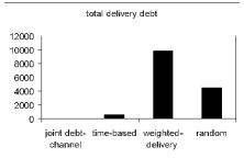
(a)

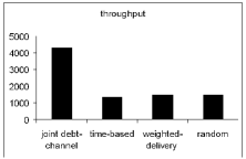
(b)

Figure 3: Performance for VoIP traffic under time-varying channels.

For MPEG traffic, we assume there are two groups of clients, with the same traffic patterns and delivery ratio requirements as those in the previous section. We use 802.11a with a fixed data rate of 54 Mb/s as the underlying MAC. The mean duration when the channel is in the bad state is 500 msec for all clients, and the mean duration in the good state is assumed to be $1+0.5n$ sec for the $n^{th}$ client in each group. There are 4 clients in both groups.

Simulation results are shown in Figure 4. As in the case of VoIP traffic, the joint debt-channel policy incurs very small total delivery debt while all the other policies have significantly higher total delivery debts. This result suggests that the simple modifications of the two largest debt first policies do not work under time-varying channels. Also, by only scheduling real-time clients with positive delivery debts, the joint debt-channel policy achieves higher throughput for the client with non-real time traffic.

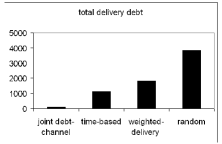
(a)

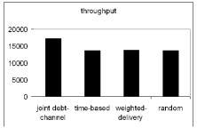
(b)

Figure 4: Performance for MPEG traffic under time-varying channels

X-C Heterogeneous Delay Bounds

Now, we study the scenario where the channel state is static but clients require different delay bounds. Since the length of a period for MPEG traffic is too small, we only simulate VoIP. There are two groups of clients. All clients generate traffic at rate 64 kbits/sec, and thus each of them has a packet in each period. Clients in group $A$ require 90$\%$ delivery ratio, with delay bounds equal to the period length. Clients in group $B$ require $50\%$ delivery ratio, with delay bounds equal to two-thirds of the period length, or 22 time slots. The channel reliability for the $n^{th}$ client in group $A$ is $(84+n)\%$, and that for the $n^{th}$ client in group $B$ is $(29+n)\%$.

Simulation results are shown in Figure 5. The adaptive allocation policy has the smallest total delivery debt. This is because the other policies, especially the two largest debt first policies, do not consider heterogeneous delay bounds at all. It is not difficult to see that, to maximize the capacity of the system, a policy should, in some sense, work in an “earliest deadline first” fashion. Without considering heterogeneous delay bounds, the largest debt first policies may unwisely schedule clients with longer delay bounds before those with shorter delay bounds, and thus result in poor channel utilization. On the other hand, such poor channel utilization will result in a large number of idle time slots. Thus, the throughputs for the non-real time traffic under these policies are higher than those for the adaptive allocation policy.

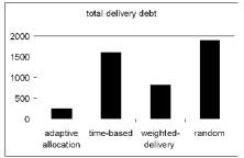
(a)

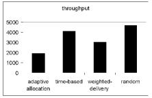
(b)

Figure 5: Performance for VoIP traffic under heterogeneous delay bounds

XI Conclusion

We have analytically studied the problem of scheduling real-time traffic over wireless channels. We have extended the model used in [10] to unreliable wireless channels and real-time application requirements, including traffic patterns, delay bounds, and timely-throughput bounds. We have developed a general class of polices that are feasibility optimal. This class can serve as a guideline for designing computationally tractable feasibility optimal policies. We have demonstrated the utility of the class by deriving scheduling policies for a general case when rate adaptation is employed and two special cases when it is not, time-varying channels and heterogeneous delay bounds. Simulation results show that the policies outperform policies described in [10]. Thus we have shown not only that the policy class is useful in designing scheduling policies, but also that neglecting some realistic and complicated settings can result in unsatisfactory policies.

References

- [1] M. Andrews, K. Kumaran, K. Ramanan, A. Stolyar, P. Whiting, and R. Vijayakumar. Providing quality of service over a shared wireless link. IEEE Communications Magazine, 39(2):150–154, 2001.
- [2] P. Bhagwat, P. Bhattacharya, A. Krishma, and S. K. Tripathi. Using channel state dependent packet scheduling to improve TCP throughput over wireless LANs. Wireless Networks, 3(1):91–102, 1997.
- [3] Y. Cao and V.O.K. Li. Scheduling algorithms in broadband wireless networks. Proceedings of the IEEE, 89(1):76–87, 2001.
- [4] E. O. Elliot. Estimates of error rates for codes on burst-noise channels. Bell Syst. Tech. J., 42:1977–1997, 1963.
- [5] I. V. Martin F., J.J. Alins-Delgado, M. Aguilar-Igartua, and J. Mata-Diaz. Modelling an adaptive-rate video-streaming service using Markov-rewards models. In Proc. of QSHINE, pages 92–99, 2004.
- [6] H. Fattah and C. Leung. An overview of scheduling algorithms in wireless multimedia networks. IEEE Wireless Communications, 9(5):76–83, 2002.
- [7] E. N. Gilbert. Capacity of a burst-noise channel. Bell Syst. Tech. J., 39:1253–1265, 1960.
- [8] A. Grilo, M. Macedo, and M. Nunes. A scheduling algorithm for QoS support in IEEE802.11 networks. IEEE Wireless Communications, 10(3):36–43, 2003.
- [9] I-H. Hou, V. Borkar, and P.R. Kumar. A theory of QoS for wireless. In Proc. of IEEE INFOCOM, 2009.
- [10] I-H. Hou and P.R. Kumar. Admission control and scheduling for QoS guarantees for variable-bit-rate applications on wireless channels. In Proc. of ACM MobiHoc, pages 175–184, 2009.
- [11] ITU-T. Pulse Code Modulation (PCM) of voice frequencies. ITU-T Recommendations, 1988.
- [12] ITU-T. G.729 based Embedded Variable bit-rate coder: An 8-32 kbit/s scalable wideband coder bitstream interoperable with G.729. ITU-T Recommendations, 2006.
- [13] L.J. De la Cruz and J. Mata. Performance of dynamic resources allocation with QoS guarantees for MPEG VBR video traffic transmission over ATM networks. In Proc. of GLOBECOM, pages 1483–1489, 1999.
- [14] Q. Liu, X. Wang, and G.B. Giannakis. A cross-layer scheduling algorithm with QoS support in wireless networks. IEEE Trans. on Vehicular Technology, 55(3):839–847, 2006.
- [15] M. Neely. Delay analysis for max weight opportunistic scheduling in wireless systems. In Proc. of Allerton Conf.
- [16] V. Raghunathan, V. Borkar, M. Cao, and P.R. Kumar. Index policies for real-time multicast scheduling for wireless broadcast systems. In Proc. of IEEE INFOCOM, pages 1570–1578, 2008.
- [17] S. Shakkottai and R. Srikant. Scheduling real-time traffic with deadlines over a wireless channel. Wireless Networks, 8(1):13–26, 2002.
- [18] L. Tassiulas and A. Ephremides. Dynamic server allocation to parallel queues with randomly varying connectivity. IEEE Trans. on Information Theory, 39(2):89–103, 1993.
- [19] H.S. Wang and N. Moayeri. Finite-state Markov channel – a useful model for radio communication channels. IEEE Trans. on Vehicular Technology, 44(1):163–171, 1995.