Spectra and Light Curves of Failed Supernovae

Abstract

Astronomers have proposed a number of mechanisms to produce supernova explosions. Although many of these mechanisms are now not considered primary engines behind supernovae, they do produce transients that will be observed by upcoming ground-based surveys and NASA satellites. Here we present the first radiation-hydrodynamics calculations of the spectra and light curves from three of these “failed” supernovae: supernovae with considerable fallback, accretion induced collapse of white dwarfs, and energetic helium flashes (also known as type .Ia supernovae).

1 Introduction

Supernovae (SNe) and gamma-ray bursts (GRBs) are among the brightest transients in the universe. As such, they have been well-studied, both observationally and theoretically. Although many theoretical models have been proposed to explain the engines behind these explosions, astronomers have focused on a few, best-fitting “standard” models. The rest of the models were, for the most part, discarded because either the engine, when studied in more detail, could not explain the observed SN characteristics (e.g. the explosion was weaker than that needed to explain most supernovae or gamma-ray bursts) and/or the rate of explosions was below the observed SN or GRB rate.

These “failed” supernovae have been neglected: very few studies have focused on their explosions and virtually no studies have calculated the emission from the explosions. With their typically dimmer outbursts and often lower rates, these objects were unlikely to have a large presence in past supernova surveys. But current (Palomar Transient Factory, PanSTARRS) and upcoming (SkyMapper, VLT Survey Telescope, One Degree Imager, Large Synoptic Survey Telescope) transient surveys are likely to actually observe these neglected transients. In this paper, we present some of the first spectra and light curves from radiation-hydrodynamics models of a few of these transients to both help guide searches and use the observations of the transients to constrain our understanding of the explosions.

The emission from explosions is powered by two primary sources: the decay of radioactive elements produced in the explosion and shock heating as the ejecta blows through the medium surrounding it. These two energy sources play varying roles in supernovae and GRBs. We believe that shock heating (albeit through shock acceleration mechanisms) powers the emission in GRBs (e.g. Meszaros & Rees (1992)). Fryer et al. (2006a) found that even the GRB-associated supernova could well be dominated by shock heating. For supernovae, the dominant energy source depends on the class, or type, of supernovae: the decay of radioactive ⁵⁶Ni and its daughter products dominates the type Ia emission but for many type Ib/c and II supernovae, shock heating can dominate the emission at peak (e.g. Frey et al. 2009, in preparation). The radiation-hydrodynamics calculations in this paper allow us to include both power sources and determine the crucial conditions behind the observed emission of these explosions.

Many transients also are sources of gravitational wave (GW) and neutrino emission. They exhibit different features form normal supernovae and these differences can be used to help us understand both explosion mechanisms better. Neutrino and GW observations of failed supernovae provide complementary (and, in some cases, stronger) probes of nuclear physics and general relativity.

In this paper, we study 3 “failed” supernova models: accretion induced collapse (AIC) of a white dwarf (Chapter 3), dim supernovae produced by fallback (Chapter 4), and type .Ia supernovae (Chapter 5). We review the engine and its environment, estimate the occurrence rate, show spectral and light-curve results from radiation-hydrodynamics calculations (using the RAGE supernova emission code—see Chapter 2) of these explosions, and discuss the neutrino and GW emission for each of these explosions.

2 Code Description

To include shock heating in our light-curve calculations, we must couple our radiation transport calculation with a hydrodynamics package. For our radiation-hydrodynamics calculations, we use the multidimensional radiation-hydrodynamics code RAGE (Radiation Adaptive Grid Eulerian), which was designed to model a variety of multimaterial flows (Baltrusaitis et al., 1996). The conservative equations for mass, momentum, and total energy are solved through a second-order, direct-Eulerian Godunov method on a finite-volume mesh (Gittings et al., 2008). It includes a flux-limited diffusion scheme to model the transport of thermal photons using the Levermore-Pomraning flux limiter (Levermore & Pomraning, 1981). RAGE has been extensively tested on a range of verification problems (Holmes et al., 1999; Hueckstaedt et al., 2005) and applied to (and tested on) a range of astrophysics problems (Herwig et al., 2006; Coker et al., 2006; Fryer et al., 2007a, b), including the strong velocity gradients that exist in supernova explosions (Lowrie & Rauenzahn, 2006).

The RAGE code can be used in 1, 2, and 3 dimensions with spherical, cylindrical and planar geometries in 1-dimension, cylindrical and planar geometries in 2-dimensions, and planar geometries in 3-dimensions. For this paper, we limit our analysis to 1-dimensional, spherical calculations. RAGE uses an adaptive mesh refinement technique, allowing us to focus the resolution on the shock and follow the shock as it progresses through the star. Even so, we were forced to regrid in the calculations to ensure that the shock was resolved (typically with coarse-grid cell sizes set to a few percent of the shock position and fine grid cell sizes set to a fraction of a percent) at early times but still allow us to model the shock progression out to 40–100 d (the shock moves from $10^{9}$ cm out to $10^{16}$ cm in the course of a simulation).

For most of our calculations, the energy released from the decay ⁵⁶Ni and ⁵⁶Co is deposited directly at the location of the ⁵⁶Ni using the following formula:

$$dE/dt=E_{\rm Ni}/\tau_{\rm Ni}e^{-t/\tau_{\rm Ni}}+E_{\rm Co}/(\tau_{\rm Co}-\tau_{\rm Ni})[e^{-t/\tau_{\rm Co}}-e^{-t/\tau_{\rm Ni}}]$$ (1)

where $E_{\rm Ni}=1.7$ MeV and $E_{\rm Co}=2.9$ MeV are the mean energies released per atom for the decay of ⁵⁶Ni and ⁵⁶Co, respectively, and $\tau_{\rm Ni}=7.6\times 10^{5}$ s, $\tau_{\rm Co}=9.6\times 10^{6}$ s. Especially at late times, this energy is not deposited into the matter surrounding it, but rather escapes the star.

In order to test the accuracy of the assumption of in-situ energy deposition, we have run a single simulation including the transport of the gamma-rays emitted during the decay of ⁵⁶Ni and its daughter product ⁵⁶Co. These results are compared with our local deposition models. To solve the transport equation in this calculation, we use the discrete ordinates “$S_{N}$” method (Wick 1943; Chandrasekhar 1950, Carlson 1955). In the spherical, 1-dimensional calculations used here, we discretize the angular variables as:

$$\frac{1}{c}\frac{\partial I_{n}(r,\nu)}{\partial t}+\frac{\mu_{n}}{r}\frac{\partial r^{2}I_{n}(r,\nu)}{\partial r}+\frac{2}{rw_{n}}\left[\alpha_{n+1/2}I_{n+1/2}(r,\nu)-\alpha_{n-1/2}I_{n-1/2}(r,\nu)\right]+$$ (2)

$$\sigma_{\rm tot}(r,\nu)I_{n}(r,\nu)=\int_{0}^{\infty}d\nu\sum_{l=0}^{L}(2l+1)\sigma_{\rm scat,l}(r,\nu)P_{l}(\mu_{n})\sum_{m}P_{l}(\mu_{m})I_{m}(r,\nu)w_{m}+Q_{n}(r,\nu)$$

where $c$ is the speed of light, $I_{n}(r,\nu)$ is the angular intensity as a function of space coordinate $r$ and photon energy $\nu$, $\mu_{n}=\cos\theta_{n}$ is the discretized $\mu$ and is taken from the abscissas of the standard 1-dimensional Gauss Legendre quadrature with $w_{n}$ the weights of this quadrature, $\alpha_{n+1/2}=\alpha_{n-1/2}-\mu_{n}w_{n}$ is the angular differencing coefficient (with $\alpha_{1/2}=0$), $\sigma_{\rm tot}(r,\nu)$ is the macroscopic total cross-section, $\sigma_{\rm scat,l}(r,\nu)$ is the $l^{\rm th}$ Legendre moment of the differential scattering cross-section, $P_{l}(\mu_{n})$ is the Legendre polynomial of $l^{\rm th}$ order and $Q_{n}(r,\nu)$ is our discretized source arising from the radioactive decay. The energy-dependent variable is discretized using standard multi-group theory (we use 12 groups). Spatial and angular cell edges are related to their respective cell centers by the standard diamond difference approach and time integration is done using Crank-Nicholson. The transport operator is inverted using a space-angle sweep, one energy group at a time. The multi-group cross-section data comes from the Los Alamos MENDF6 library (Little, 1996).

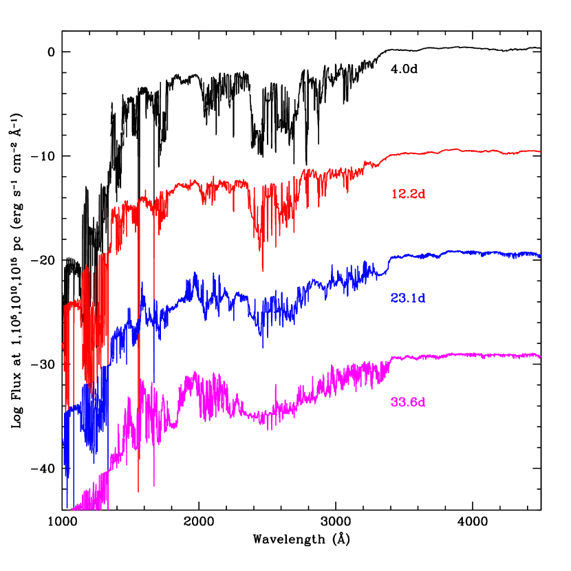
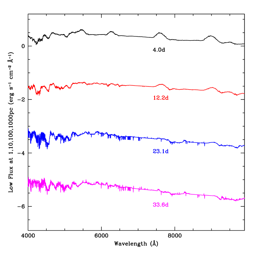
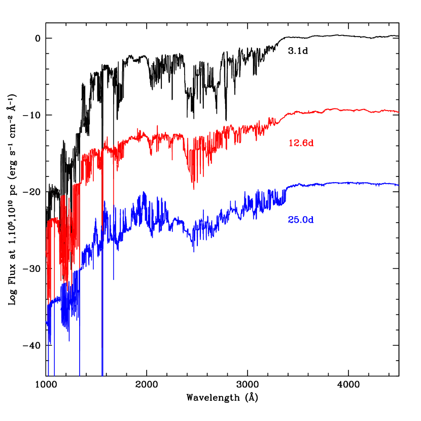
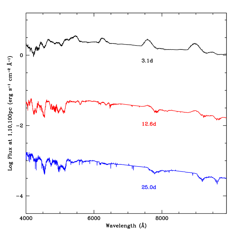
Figure 1: Flux versus wavelength for a 16 M_⊙ binary progenitor (collapsing as a Wolf-Rayet star of less than 5 M_⊙) at 4 different times after the launch of the explosion. The high energy spectra are separated each by 10 orders of magnitude to show the full structure of each spectrum. We have effectively put the different models and different distances: 1 pc, 10⁵ pc, 10¹⁰ pc and 10¹⁵ pc. The corresponding fluxes at low energy, which have much less dramatic structures, are separated by 2 orders of magnitude. The top two panels show the spectra for in-situ gamma-ray deposition. The bottom two panels show the resulting spectra using our gamma-ray transport algorithm. At these times, the differences are minimal. Indeed, our tests show that even for a type Ia supernova, gamma-ray transport is not critically important until well after 60 d.

For the comparison of our in-situ gamma-ray deposition to that of transport, we model a Wolf-Rayet star. The spectra for our in-situ gamma-ray deposition and transported gamma-ray calculations are shown in Figure 1. At these early times, the two calculations are identical. The mean free path of gamma-rays remains small for this model, and most of the models studied in this paper, for roughly 60 d (longer for some), so the fact that in-situ deposition is a good approximation is not surprising. The one exception is our low density .Ia model. In this .Ia model, the gamma-rays emitted by the decay ⁵⁶Ni are not trapped after $\sim$15 d. We discuss these results further in section 5.

For opacities, our radiation hydrodynamics calculations consider a single group using the Rosseland mean opacity for the diffusion coefficient and the Planck mean opacity for the emission/absorption terms in the transport equation. These gray opacities are obtained from the LANL OPLIB database (Magee et al. 1995; http://www.t4.lanl.gov/cgi-bin/opacity/tops.pl) and have been extensively used in astrophysics modeling, including many problems in supernovae (e.g. Fryer et al. 1999b; Deng et al. 2005; Mazzali et al. 2006). This opacity database is continually updated, and we use the most recently produced opacity data in all of our calculations. The opacities made available in this database are computed under the assumption that the atomic populations are in local thermodynamic equilibrium at the material temperature. Thus, the opacity can be determined assuming a single temperature in each cell.

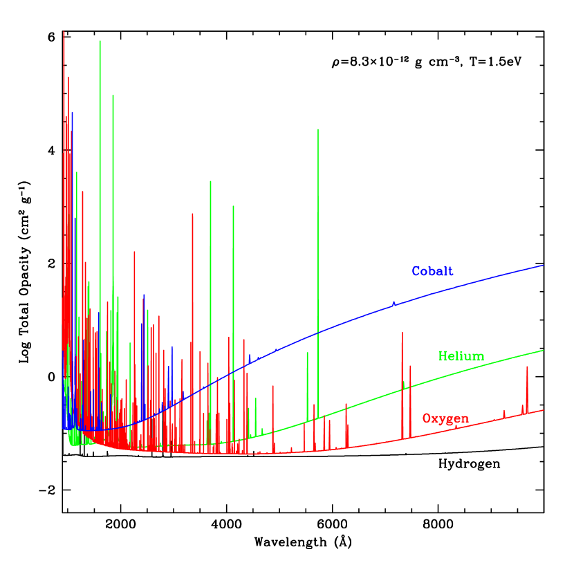
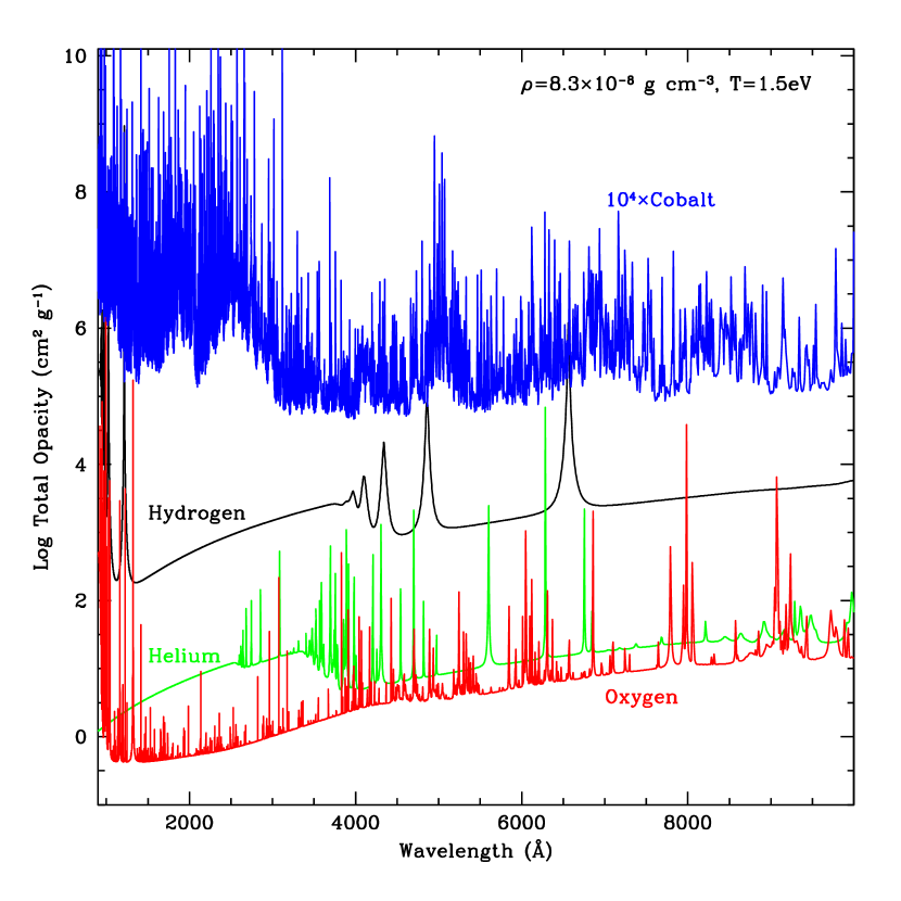
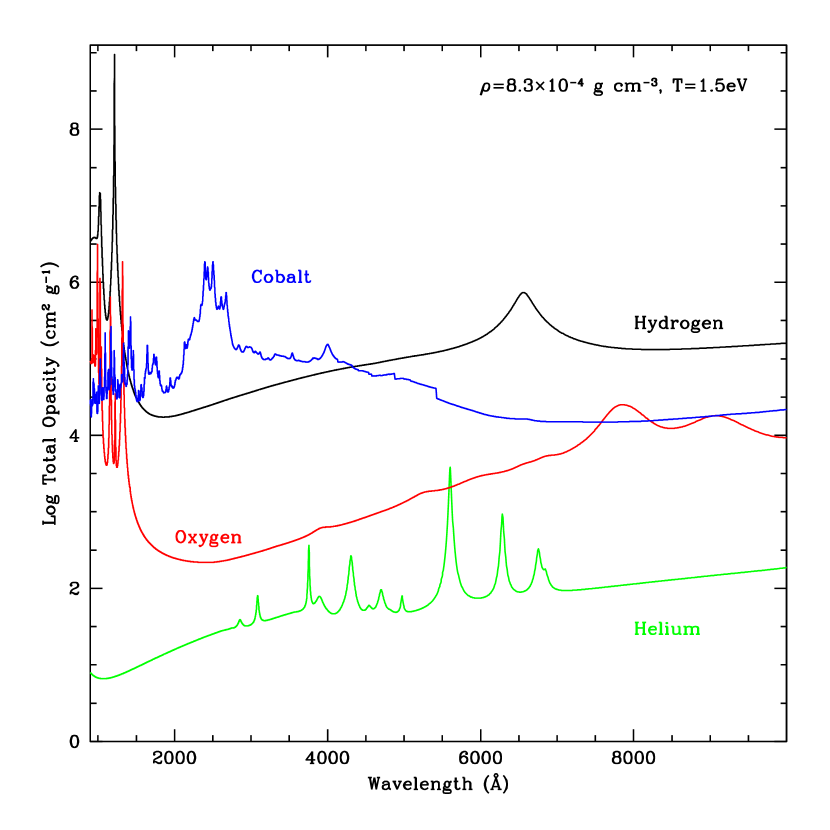
Figure 2: Opacities for hydrogen, helium, oxygen and cobalt versus wavelength for 3 different density/temperature pairs relevant to our supernova explosion. The high density plot ($8.3\times 10^{-4}$ g cm^-3) is a typical density near the time of shock break-out. Under these conditions, the hydrogen opacity is quite large (3 orders of magnitude higher than the equivalent helium opacity) and many lines are blended for each material. At lower densities, $8.3\times 10^{-8}$ g cm^-3, the lines dominate the opacities. The Doppler shifts in the exploding star are easily sufficient to cause these lines to blend. At still lower densities, the opacities are quite low and the iron peak material has considerably fewer lines.

As an illustration of the opacities used in our calculations, we have plotted the opacity values from the LANL OPLIB database for a variety of pure elements at 3 different density/temperature pairs (Fig. 2). At low densities, we note that hydrogen in local thermodynamic equilibrium will be completely ionized, even at temperatures as low as 1eV, because the effect of three-body recombination is suppressed relative to that of photoionization. Thus, bound-bound features associated with the hydrogen atom, such as the H$\alpha$ line, are not expected to be present under these conditions. The pure elemental opacities are subsequently combined in the appropriate ratios for each cell that is considered in the calculation. Figure 3 shows 3 different density/temperature pairings for the composition of the surrounding wind medium used in our fallback model.

With our radiation-hydrodynamics calculations, we calculate the temperature structure of the matter in the exploding star as a function of time. Unlike post-process calculations based on purely hydrodynamic models, we can use this matter temperature profile in a post-process approach to determine the full time-dependent spectra from this supernova explosion. To calculate the spectrum, we first assume that each radial zone emits radiation isotropically based on its temperature and absorption coefficient:

$$L_{\nu}=m_{\rm zone}\frac{2h\sigma_{\rm abs}\nu^{3}}{c^{2}}\frac{1}{e^{\nu/T_{\rm mat}}-1}d\nu\frac{(1-v/c)^{2}}{\sqrt{1-(v/c)^{2}}}$$ (3)

where $m_{\rm zone}$ is the mass of the zone, $h=6.626\times 10^{-27}{\rm ergs}$ is Planck’s constant, $c$ is the speed of light, $v$ is the velocity of that zone, $(1-v/c)^{2}/\sqrt{1-(v/c)^{2}}$ is the time dilation effect on the luminosity, $\sigma_{\rm abs}$ is the absorption cross-section (which depends on composition, temperature and density), $\nu$ is the frequency ($d\nu$ is the size of the frequency bin), and $T_{\rm mat}$ is the matter temperature (note that in the exponential, $\nu$ and $T_{\rm mat}$ must have the same units—e.g. $h\nu/k_{\rm Boltzmann}T_{\rm mat}$).

This equation gives us the emission in each zone, but what we really want is the emission directed toward an observer in a single direction. In order to calculate both accurate mean free paths through the spherically symmetric zones (to get limb effects) and the correct Doppler shifts, we have discretized each zone into angular bins (Fig. 4). For our calculations, we use 40 angle bins. The observed spectrum is then:

$$L^{\rm tot}_{\nu}=\sum_{\rm zone}\sum_{\rm angle}L_{\nu}^{{\rm angle,zone}}e^{-\tau^{{\rm angle,zone}}}$$ (4)

where $\tau^{\rm angle,zone}$ includes both Doppler effects (everything is calculated in the rest frame of the observer) and geometric or limb effects. $L_{\nu}^{\rm angle,zone}$ is now the emission based on the mass in our angular bin ($m_{\rm zone,l}$) pointed in the observers direction:

$$L_{\nu}=\frac{m_{\rm angle,zone}}{n_{\rm angular\,bins}}\frac{2h\sigma_{\rm abs}\nu^{3}}{c^{2}}\frac{1}{(e^{\nu/T_{\rm mat}}-1)}d\nu\frac{(1-v/c)^{2}}{\sqrt{1-(v/c)^{2}}}$$ (5)

where $n_{\rm angular\,bins}=40$ in our case. As long as our assumption holds concerning the accuracy of the matter temperature obtained from our radiation-hydrodynamics calculation, this semi-analytic post-process gives us an accurate calculation of the emission. We then can calculate the emission over our entire energy grid consisting of 14,900 groups from roughly $10^{-3}$ eV to $10^{4}$ eV (the grid depends upon the temperature and density of the matter). For typical supernova temperatures and densities, we generally have $\sim 13,000$ groups lying between 1000 and 10,000 Å.

To obtain optical and UV light curves over the wavelength range 1600-6000Å, , we need to integrate our spectrum over a band filter. In our case, we use the SWIFT band filters for U, B, and V (Gehrels et al 2004; Roming et al. 2005; Poole et al. 2008): swuuu_20041120v104.arf, swubb_20041120v104.arf, and swuvv_20041120v104.arf to be specific. We also include the data for the swuw1_20041120v104.arf, swuw2_20041120v104.arf, and swum2_20041120v104.arf UV bands.

3 Accretion Induced Collapse

When accretion onto a white dwarf pushes its mass above the Chandrasekhar limit, the star begins to compress. This compression can lead to one of two fates. In one scenario, nuclear burning releases enough energy to completely unbind the star in a thermonuclear explosion, producing the well-known type Ia supernova used to probe the early universe. In the other, the white dwarf collapses down to a neutron star (accretion induced collapse or AIC). The gravitational potential energy released in this collapse also produces an explosion. It is this latter, lesser-known, accretion induced collapse that we study here. An accretion induced collapse can only form if nuclear burning during the collapse does not inject enough energy to unbind the star. If the core of the white dwarf is cool enough such that nuclear burning does not occur (or is weak) until after the core has imploded (and lost energy through neutrino emission), nuclear burning will be unable to unbind the star.

Nomoto & Kondo (1991) summarized the fate of an accreting white dwarf based on its composition (carbon-oxygen versus oxygen-magnesium-neon white dwarf), initial mass, and accretion rate. They argued that white dwarfs with initial masses above 1.2M_⊙ are likely to form AICs. Unless the accretion rate is quite low ($<10^{-6}$M _⊙ y^-1), the mass of these white dwarfs will exceed the Chandrasekhar mass well before accretion energy can heat the core. The fact that many of these massive white dwarfs are OMgNe white dwarfs whose cores are cooled by Urca processes (the emission of a neutrino and anti-neutrino pair within a nucleus) does not help. They also argued that AICs are formed when the accretion rate is high, again causing the white dwarf mass to exceed the Chandrasekhar limit before the core is heated by this accretion. With these two constraints, we can study the rates of AICs.

Note that an accretion induced collapse has many properties similar to that of electron capture supernovae. An electron capture supernova is produced in an AGB star with a mass placing its evolution at the boundary between mass ejection (forming a white dwarf) and further core nuclear burning producing an iron core and, ultimately, a iron core-collapse supernovae (see Wheeler et al. (1998),Wanajo et al. (2003), and Poelarends et al. (2008)). An electron capture supernova is produced in the collapse of the OMgNe core at the center of this AGB star. The details of the explosion for an electron capture supernovae are very similar to those of an AIC. The primary difference between these objects is the surrounding environment and, as we shall see, this environment plays a strong role in determining the observations of these objects. In this paper, we focus only on the surrounding environments of AICs.

3.1 Accretion Induced Collapse Rates

A number of methods have been used to constrain AIC rates. Thus far, no outburst from the accretion induced collapse of a white dwarf has been observed. Given that the outburst is expected to be very dim because shock heating is negligible and the predicted ⁵⁶Ni yields are all low, i.e. $<0.05$ M_⊙ (Fryer et al. (1999a); Kitaura et al. (2006); Dessart et al. (2007)), the lack of observed AICs does not place firm upper limits on the AIC rate. With more firm observational predictions and upcoming surveys, observations will begin to place constraints on the rates.

Theoretical estimates of the rate of AICs are also quite uncertain. A number of progenitor scenarios have been proposed, mostly in the search for the elusive progenitor to type Ia supernovae (see Livio 2001 for a review). Although single degenerate models exist, the dominant progenitor of AICs, if we accept the conclusions of Nomoto & Kondo (1991), comes from double degenerate mergers with a rate of $\sim$ 10^-2 y^-1 in a Milky-Way sized galaxy. This result depends upon a number of assumptions about the accretion evolution in these binary systems and the true rate of AICs could be many orders of magnitude lower than this value. Studies of binary mass transfer (Yoon et al. (2007); Livio (2001) and references therein) and white dwarf accretion (Fisker et al. (2006)) are both becoming more accurate. As they are coupled with stellar evolution models of these systems, this rate estimate for AICs should become more accurate.

Alternatively, one can use observed features of AIC explosions to constrain the AIC rate. By comparing observations of nucleosynthetic yields to explosion models, Fryer et al. (1999a) argued that the neutron rich ejecta from an AIC limits their rate to $\sim$ 10^-4 y^-1. More recent results, which eject a smaller fraction of neutron-rich material, may loosen this constraint by 1 order of magnitude (Kitaura et al. (2006); Dessart et al. (2007)), allowing rates as high as $\sim$ 10^-3 y^-1.

3.2 AIC Light Curves and Spectra

Recall that light curves and spectra are powered by both shock heating as the ejecta hits its surrounding medium and through the decay of radioactive elements. The standard explosion model of Fryer et al. (1999a) predicted $\sim$0.05 M_⊙ of ⁵⁶Ni ejecta. Other explosion models predict even less mass in ⁵⁶Ni. In this case, shock heating will play an equal, if not dominant, role in the light curve.

For our calculations, we use an explosion from Fryer et al. (1999a). The total explosion energy for our canonical AIC is $2\times 10^{51}$ ergs. With the low ejecta mass (0.2 M_⊙), this energy corresponds to a high average initial velocity of the ejecta ($3\times 10^{9}$ cm s^-1). The composition is also based on the explosion models of Fryer et al. (1999a), with roughly 20% of the eject in the form of ⁵⁶Ni (0.04 M_⊙). We construct a second explosion with 1/10th the amount of mass (hence 1/10th the explosion energy and 1/10th the ⁵⁶Ni yield) to compare to the lower ejecta models predicted by more recent calculations Dessart et al. (2007). A summary of the explosion energy, ejecta mass, and ⁵⁶Ni mass is shown in Table 1. On top of these explosions, we construct a surrounding environment with a density structure (Fig. 5) based on preliminary binary merger calculations by Motl et al. (in preparation).

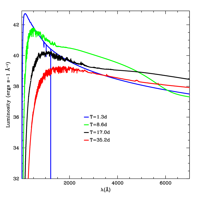
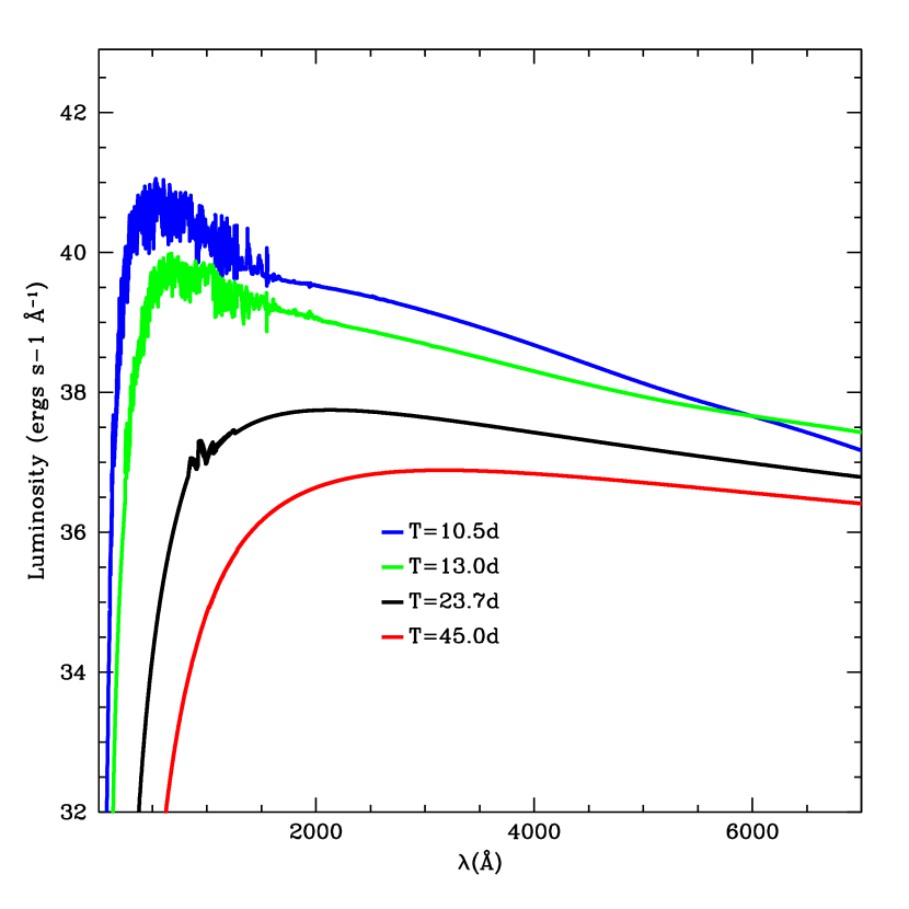
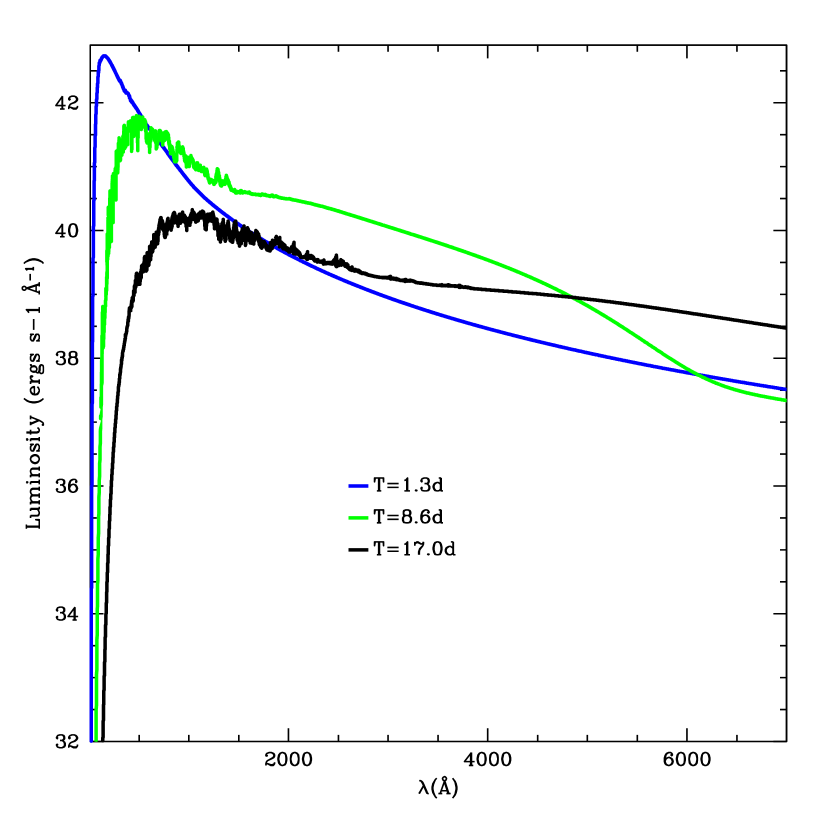
Figure 6: Snapshots in time of our AIC spectra for 3 models: The top two plots represent a large ⁵⁶Ni yield of 0.041 M_⊙ (left) and a low ⁵⁶Ni yield of 0.0041 M_⊙ (right). The lower ⁵⁶Ni yield coupled with lower energy produces a much weaker explosion. Note that the spectra peak below 1000 Å (in the X-ray). The bottom plot represents our large ⁵⁶Ni yield with CO on top of the star instead of helium. Note that, for this model, the composition on top of the explosion plays very little role in shaping the spectrum.

Due to the low envelope mass, the ejecta begin to emit within the first day of the explosion (Fig. 6). At this time, the ejecta is still hot, ionizing the material above it, leading to very few lines. Even when we place a CO atmosphere on top of the white dwarf, at early times there are very few lines due to the high peak temperature. As the ejecta expands, it cools and line features appear. But there are no strong identifying (specific to AICs) features in the spectra.

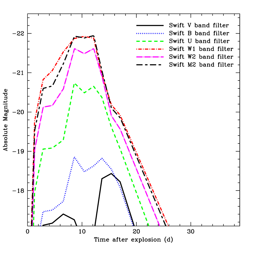
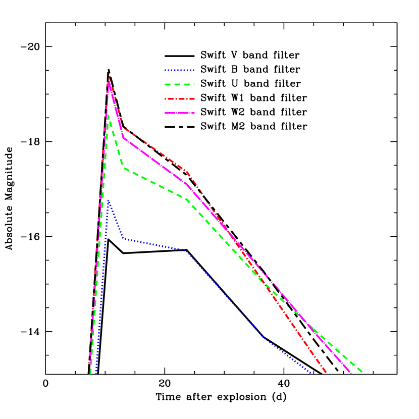
Figure 7: Light curves (absolute magnitudes as a function of time) for 5 different bands based on the Swift filters. The peak in the X-ray for these explosions means that the higher-energy bands are brightest. Although the visible magnitudes are dimmer than normal Type Ia supernovae, these supernovae are much brighter than normal Ia supernovae in the high-energy Swift W1 and W2 bands. The left panel shows our high-mass ejecta run with 0.041 M_⊙ of ⁵⁶Ni ejecta. The right panel shows the light curves for our low-mass ejecta run (0.0041 M_⊙ of ⁵⁶Ni ejected).

The light curves in V and B bands peak at roughly 15 d with peak absolute magnitudes of -18.5 to -19 magnitudes (close to that of supernovae) for our standard model (Fig. 7). The drop is fairly rapid, and by 30d, the absolute magnitude for both these bands is below -17. The peak in the U and Swift UV bands is bright (as we might expect from the high effective temperatures of the spectra).

For our lower yield model, the combined lower energy and lower mass of ⁵⁶Ni ejected lowers the AIC emission. The peak absolute V and B magnitudes of our low-density run do not exceed -16 and by 40 d are below -14. At early times, there are a number of lines in the UV, but by 20 d, the low density and high temperature of this model ionizes most of the material and the spectra are fairly featureless.

3.3 Neutrinos and Gravitational Waves from AICs

The collapse and bounce of an AIC is very similar to that of a normal supernova (see Fryer & New 2003 for a review). As such, both the neutrinos and GW emission should be similar to that of core collapse. The primary difference is that the explosion is likely to happen quickly and there is unlikely to be much, if any, material falling back onto the newly formed neutron star. For neutrinos, this means that the explosion is clean, allowing a clear view of a cooling neutron star. For gravitational waves, there will be no strong signal from convective instabilities above the proto-neutron star. But there is a possibility that AICs will have high angular momenta at collapse. As such, the AIC scenario is a leading candidate among stellar collapse to form bar-mode (and related) instabilities.

4 Fallback Supernovae

Standard core-collapse supernovae are the explosions produced when the iron cores of stars more massive than 8–10 M_⊙ collapse to form neutron stars. The potential energy released in this collapse drives an explosion. But not all stellar collapses form strong supernova explosions. The explosion launched in the stellar core moves out through the star and decelerates as it pushes out the rest of the star. For some of the initial exploding material, this deceleration drops the explosion energy below the escape energy from the core. This material ultimately falls back onto the neutron star.

Fryer (1999) argued that although this “fallback” is only a few tenths of a solar mass for 15 M_⊙ stars, it might be several solar masses for 25 M_⊙ stars. Based on their understanding of fallback, Fryer & Kalogera (2001) argued for a range of neutron star and black hole masses. One of the successes of the current supernova mechanism is its prediction of fallback and a broad range of remnant masses. But fallback also has implications for supernova light curves. ⁵⁶Ni is produced in the innermost ejecta. This ejecta is the first material to fall back and if the fallback is extensive, very little ⁵⁶Ni will be ejected to power the supernova emission. In addition, fallback tends to occur in weaker explosions, reducing the emission energy from shocks as well. So fallback supernovae will have a range of peak emission, from energies as strong as classic supernovae when little fallback occurs down to unobservable whimpers when the fallback is extensive.

The fate of the core changes if fallback is so large that it pushes the neutron star beyond the maximum neutron star mass. These systems collapse to form a black hole. For this paper, we will focus on the emission of black-hole-forming, fallback supernovae.

4.1 Fallback Rates

In current simulations, the energy produced in the convective engine decreases for stars more massive than 20 M_⊙ while the binding energy of the star increases dramatically at roughly this same mass point. Including large errors in the explosion energies, Fryer & Kalogera (2001) were able to pinpoint the transition mass from neutron star and black hole formation to stars with initial masses within the 18–23 M_⊙ range. Fryer & Kalogera (2001) found that, within the uncertainties, the formation rate of black holes in supernova explosions was somewhere between 10–40% that of the total supernova rate. The largest uncertainty in this estimate is the initial mass function. Winds can allow the formation of neutron stars by more massive, solar metallicity stars (above $\sim 60$ M_⊙), but this does not affect the rate significantly.

4.2 Fallback Spectra and Light Curves

For our calculations, we use a 40 M_⊙ binary progenitor for Cas A (Fragos et al. 2008). In this star, we drive a $2\times 10^{51}$ erg explosion. The binding energy of this star is much greater than $2\times 10^{51}$ ergs and the final remnant mass after fallback is 4.5 M_⊙. With this much fallback, very little ⁵⁶Ni is ejected: $<2\times 10^{-13}$ M_⊙. A summary of the explosion energy, ejecta mass, and ⁵⁶Ni mass is shown in Table 1. On top of this explosion, we construct two surrounding environments with density structures (Fig. 8): one based on binary mass ejection (100 km s^-1 velocity, $\dot{M}=1$ M_⊙ y^-1) and one with a small atmosphere ($<0.00054\,M_{\odot}$) topped by a wind profile (1000 km s^-1 velocity, $\dot{M}=10^{-5}$ M_⊙ y^-1).

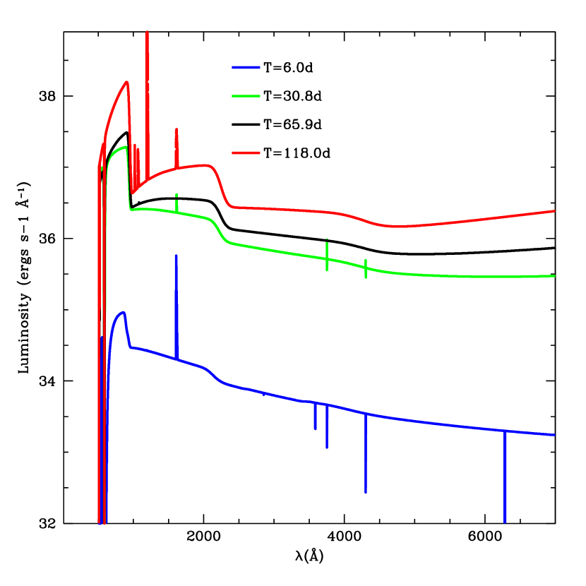
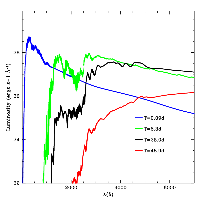
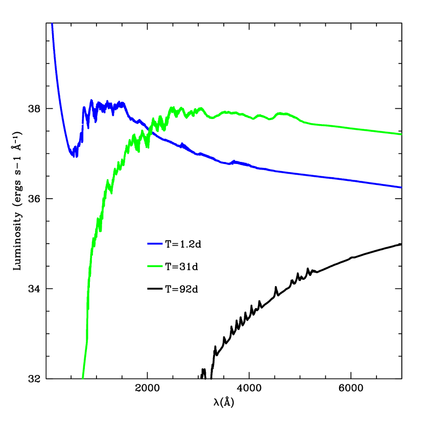
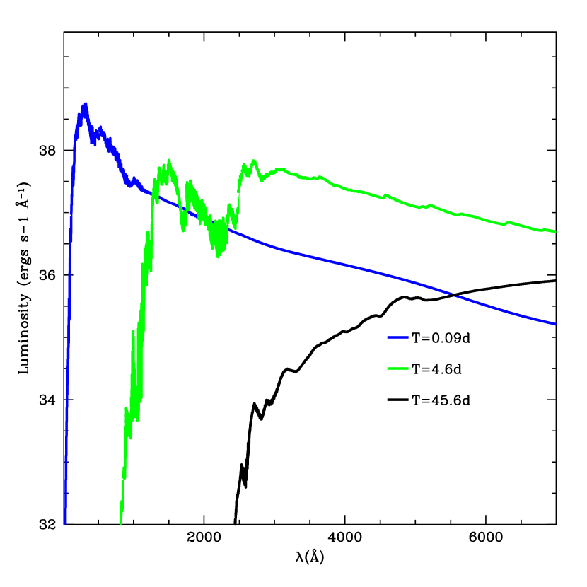
Figure 9: Spectra from our extremely dense and dense surrounding medium models of supernova fallback. In the more dense case, the outburst is still peaking 100 d after the launch of the explosion and strong emission/absorption lines are evident. The lines, dominated by material ahead of the ejecta, are narrow. In the lower density case, the peak occurs much sooner and lines are part of the ejected material and hence are broader. The bottom, left plot shows the lower density case using 5 groups for the radiation transport. The additional groups lead to a slightly different temperature profile that can change the spectra dramatically. But the peak fluxes are not altered significantly. The bottom right plot shows the results using twice the coarse-bin resolution and 10 times the fine (AMR) resolution. The spectra are nearly identical to its comparable low resolution case (dense surrounding medium).

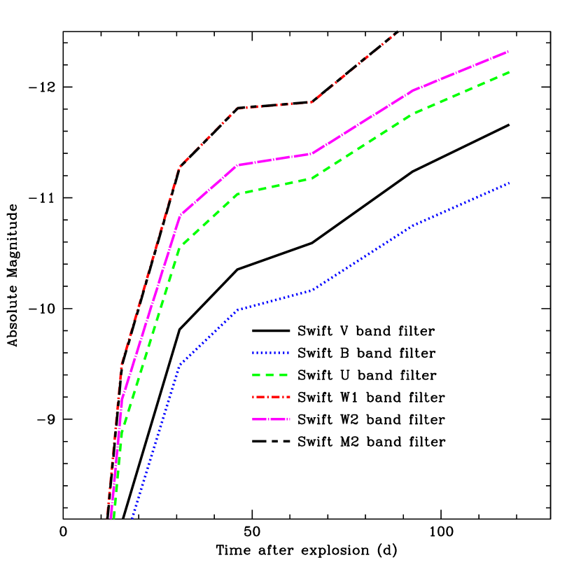
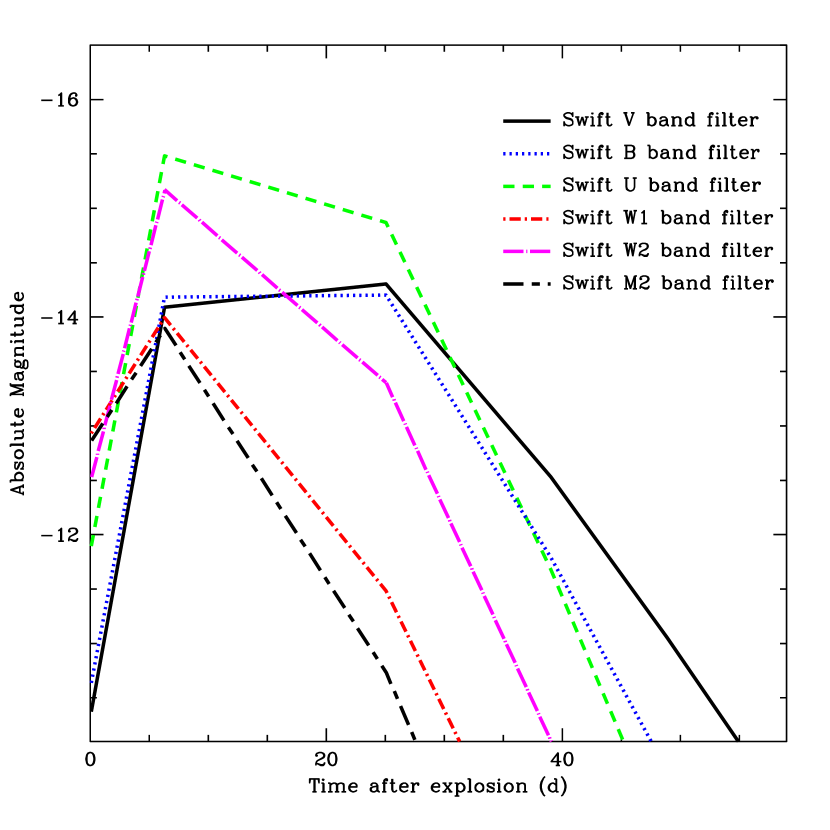
Figure 10: In the extremely dense surrounding medium model (left panel), the light curve is still rising after 100 d. In the less dense case (right panel), the light curve peaks after 15 d, but is 3 magnitudes brighter than the projected peak in our dense model.

The large mass in the binary mass ejection case, coupled to the weak explosion energy, delays shock breakout until after the ejecta loses much of its energy (Figs. 9,10). In this simulation, the explosion has yet to peak, even 100 d after the explosion. But it will peak at very low V, B magnitudes (below absolute magnitudes of -13). This is an extreme case, where the environment is very dense out to $10^{16}$ cm due to a binary mass ejection just prior to collapse.

More likely, the mass ejection phase is followed by a Wolf-Rayet wind phase. Even with this lower-density surrounding medium, the low ejecta velocity coupled to its low ⁵⁶Ni ejecta produces a very weak explosion with peak V, B absolute magnitudes of -15 (Figs. 9,10). The lower density means the peak emission occurs quickly ($\sim$10 d) and the V-band absolute magnitude drops below -12 at about 45 d.

To test our single group approximation, we modeled a 5-group transport calculation for our diffuse case (Fig. 9). Although many of the lines are similar, the spectral fluxes can be very different. Although the peak in the light-curve doesn’t change dramatically in the V-band, the UV light-curve is very different. Ultimately, many group calculations will be required to model detailed spectral light curves.

To test our resolution, we completed 1 run with twice the coarse-bin resolution and 10 times the effective (AMR) spatial resolution (Fig. 9). The spectra from this simulation is nearly identical to our standard runs.

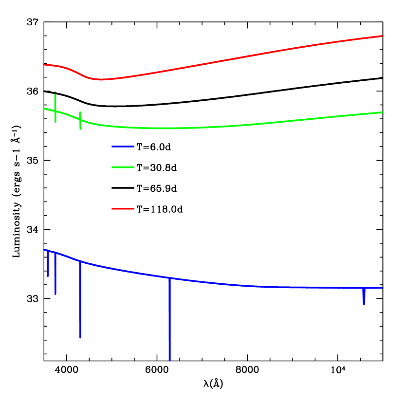
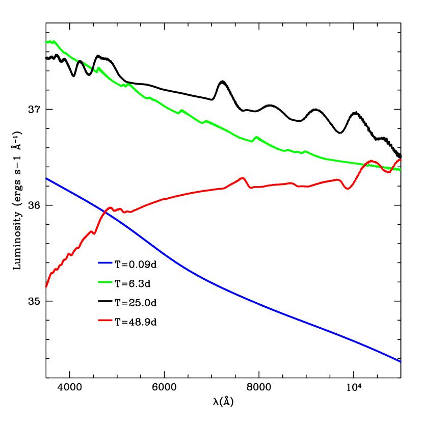
Figure 11: Optical and IR spectra of our high and low density fallback models at the same time snapshots as figure 9. In the dense model, the narrow lines are produced by material just being heated by the radiation front. First only in absorption, as the material is heated, we also see emission lines. In the less dense model, we observe the broad lines from the shocked ejecta itself.

Detailed spectra might also help to give us a better understanding of the surrounding medium. Figure 11 shows the optical/IR spectra for our two fallback models for the same snapshots in time of figure 9. Note that we assume our atomic levels are in local thermodynamic equilibrium with the radiation front. Especially for material ahead of our shock front (which is not in thermodynamic equilibrium), we overestimate the level of ionization, producing fewer lines than what may be observed. Within the shocked material, local thermodynamic equilibrium is a better assumption, and our broad lines representing this shocked ejecta are fairly accurate and provide an ideal probe of the explosion itself.

4.3 Neutrinos and Gravitational Waves from Fallback

The collapse and bounce phases of stellar collapse with considerable fallback is similar to normal supernovae. Explosions with considerable fallback are weaker explosions. In general, these explosions have longer delays between bounce and explosion. As such, the convective timescale is longer, producing a longer boiling phase prior to explosion. After the explosion, fallback accretion adds mass to the proto-neutron star, possibly causing it to collapse to form a black hole. These engines produce neutrino light curves that are much broader than normal supernovae. The total emission will be more than a factor of 2 higher than normal supernovae, primarily in an extended convective phase (during the first second) and a higher neutrino flux in the first 10 s from fallback (Fryer, 2009). Observations of this extended emission will constrain our understanding of the supernova explosion mechanism and the nature of fallback.

The extended convective phase may also develop low-mode instabilities, leading to stronger GW emission, especially through asymmetric neutrino emission (Kotake et al., 2009). If the proto-neutron star collapses to form a black hole, black hole ringing and related instabilities may occur, producing another source of GWs (see Fryer & New 2003).

5 .Ia Supernovae

Bildsten et al. (2007) have argued that faint supernova-like outbursts can occur in helium flashes of accreting material in AM Canum Venaticorum (AM CVn) binaries. In these binary systems, a C/O white dwarf is accreting from its smaller He white dwarf companion, slowly whittling away the mass of the He white dwarf. At high accretion rates, the helium accretes onto the C/O white dwarf and burns stably. The system evolves, widening the orbit, and causing the accretion rate to decrease. At sufficiently low accretion rates ($\dot{M}<2\times 10^{-6}$ M_⊙ y^-1), the burning can be unstable. The accreting white dwarf can go through a series of flashes, each increasing the entropy of the system, leading to larger ignition masses. Typically, the last “flash” will result in the largest explosion and it is this explosion that Bildsten et al. (2007) focus on as a potential transient observation.

5.1 .Ia Supernova Rates

Using the local Galactic density of AM CVn’s and assuming every AM CVn gives one explosive last flash, Bildsten et al. (2007) argued that the .Ia supernovae should occur at a rate of $6.67\times 10^{-5}-0.0002$ per year in an E/SO galaxy.

5.2 .Ia Supernova Spectra and Light Curves

For our calculations, we use a FLASH (Fryxell et al., 2000) simulation of a Type .Ia outburst. This model produced a $7\times 10^{51}$ erg explosion with 0.1 M_⊙ of ejecta. This is our fastest explosion, with mean velocities around 80,000 km s^-1. The total amount of ⁵⁶Ni ejected is 0.014 M_⊙.

On top of this explosion, we construct two surrounding environments with density structures (Fig. 12) based on binary accretion simulations (Motl et al. in preparation): one using the density profile along the binary orbital plane (higher density) and one using the profile along the orbital axis (lower density).

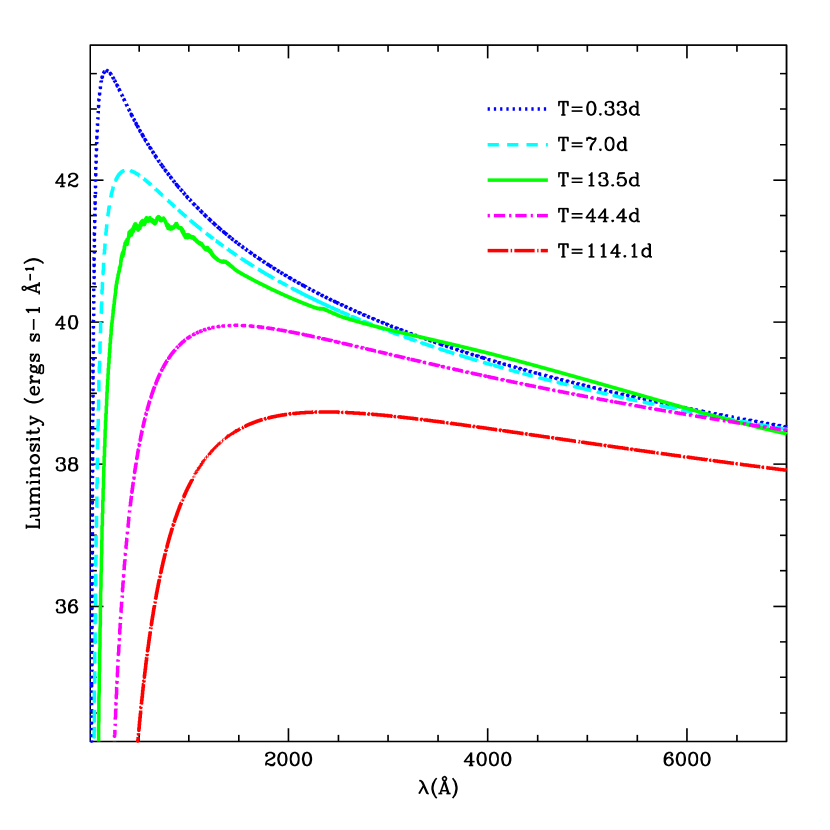
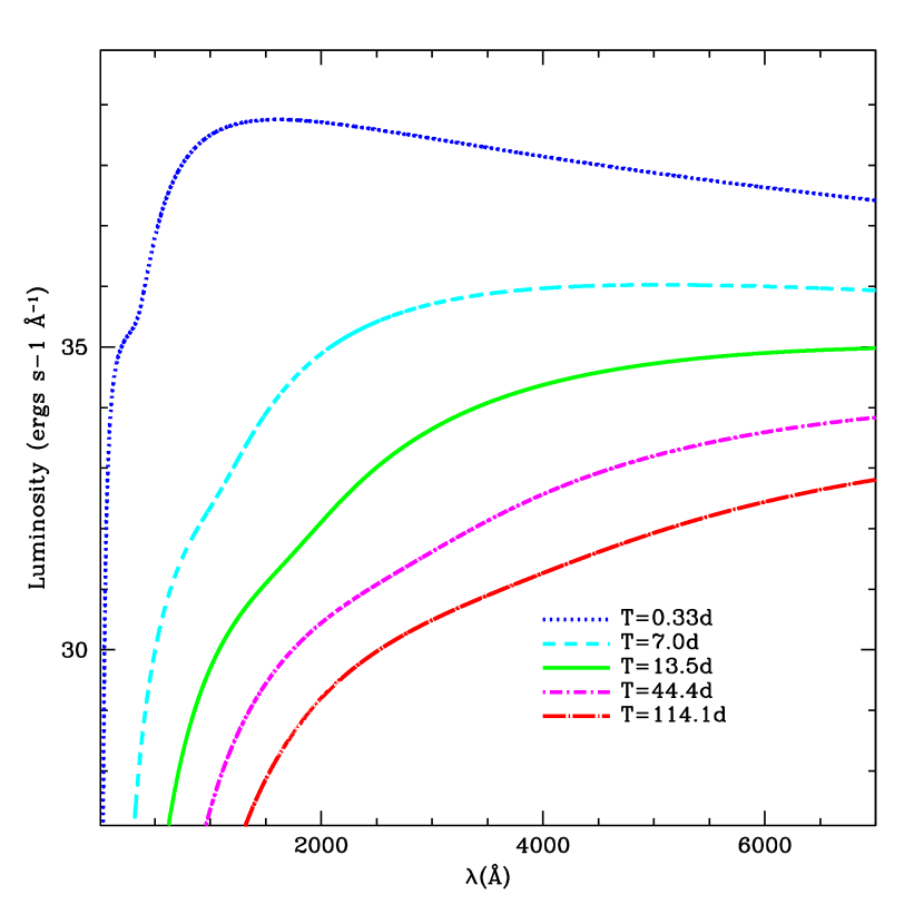
Figure 13: Spectra from our .Ia models. This fast shock in this models ionizes most of the material, producing line-free spectra. This strong shock also produces spectra that peak in the X-ray.

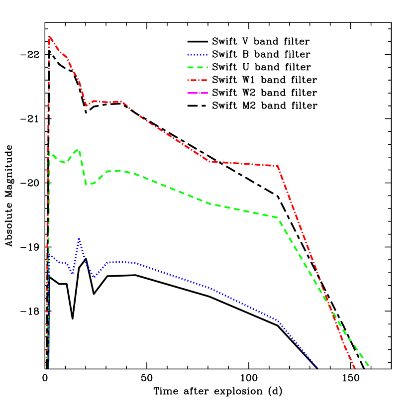
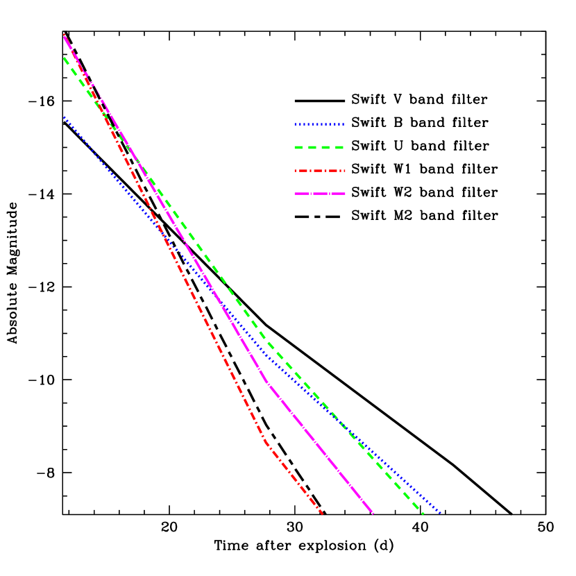
Figure 14: The light curves of our .Ia supernovae (left: high density, right: low density). Given the spectral peak in the X-ray (Fig. 13), it is not surprising that the denser (orbital plane) model is much brighter in the W1 and W2 bands than the V band. Even so, in a dense medium, .Ia supernovae are nearly as bright as their Ia counterparts. But in a diffuse medium (model based on binary interaction along the axis), the peak magnitudes are several magnitudes dimmer than type Ia supernovae.

The emission from a .Ia supernova is strongly dependent on the density profile. First, there is very little radioactive ejecta, so it does not contribute strongly to the light curve. But with the fast ejecta velocities and low masses, the gamma-rays from radioactive decay begin to stream out early, also limiting how much the gamma-rays can contribute to the light curve. Recall that we deposit our energy in-situ and hence we are overestimating the emission from this low-density case. The presence of fast moving ejecta means that shocks are important for the light curve (Fig. 14). For our dense environment, the V and B bands peak between absolute magnitudes of -18 to -19 (near to normal supernova brightnesses). The light curve will remain bright for nearly 100 d. The high shock velocities and low densities lead to high temperatures and spectra peaked in the UV and X-ray at early times (Fig. 13). In the dense model, there is a decided drop in the UV band emission after twenty days. This occurs when the radiation leading the shock emerges from ejecta and the radiation front leading the ejected shock cools. From this point on, the photosphere of the explosion resides near the density peak in the ejecta. Shock emergence is discussed in more detail by Frey et al. (in preparation).

But if the surrounding environment is diffuse, there is too little material to create strong emission, and the peak emission is limited to that of the initial explosion, peaking with absolute magnitudes around -16 and dropping below -14 before 20 d (below -12 by 30 d).

The high temperatures and low densities limit the number of lines in the emitting regions and the regions just above these emitting regions. Aside from absorption lines caused by the surrounding medium, we expect very few line features in their spectra.

5.3 Neutrinos and Gravitational Waves from .Ia Supernovae

.Ia supernovae will not be strong sources of neutrinos or GWs.

5.4 Summary

In this paper, we reviewed 3 separate explosions, providing the first radiation-hydrodynamics calculations of their emission (both spectra and light curves). Each of these explosion scenarios will ultimately require detailed, individual studies as upcoming surveys begin to make first observations. Here we have described many of the basic features one should expect in these explosions, focusing on the physics that alters the emission.

For supernovae, the emission is powered by a combination of the energy from the decay of radioactive elements (primarily ⁵⁶Ni and its daughter products) and shock heating as the ejecta moves through its surroundings. For all of these “failed supernovae”, the low ⁵⁶Ni yield coupled to the high explosion velocities lead to peak emission dominated by the shock heating. The energy from shock heating depends both on the velocity of the ejecta and the density structure of the surrounding medium. For a given explosion, its surrounding medium (strength of the stellar wind, ejecta from a binary mass transfer phase, etc.) determines the peak luminosity and also shapes the spectra. Unfortunately, neither the wind mass-loss nor the ejecta from binary mass transfer are well-known theoretically. Observations of these transients will first and foremost help us in constraining the nature of these mass ejection mechanisms.

Depending upon the environment, the accretion-induced collapse outburst could reach peak magnitudes that are nearly as bright as normal supernovae, if only for a brief time (absolute magnitude in the V band of -18.5, but dropping to below -17 by 30 d). If the total mass ejecta is at the lower limit predicted by simulations, the peak brightness will be several magnitudes dimmer than typical supernovae (V band absolute magnitude of -16). The rate of AICs could well be as high as the type Ia supernova rate, but it could be several orders of magnitude lower. If typical peak magnitudes were at the higher range, and the rate were truly close to the supernova rate, we should already have observed some of these outbursts in existing samples. The progenitors of AICs are intimately linked to the progenitors of type Ia supernovae, and understanding the AIC progenitor will teach us about this supernova progenitor. A nearby detection of an AIC will also provide insight into neutron star formation. Without the convective engine and possibility of fallback, the neutrino signal from AICs is a pristine measurement of stellar collapse and bounce. We can use the neutrino signal to study nuclear physics and the formation of the neutron star. In addition, because of the potential for rapid spinning prior to collapse, AICs are the most promising candidates for bar mode, and related, instabilities in the proto-neutron star, a strong source of GW emission. The observation, or lack thereof, of a GW signal can be used both to understand the white-dwarf accretion process and the nature of these proto-neutron star instabilities.

Type .Ia supernovae eject even less ⁵⁶Ni (and less total mass) than our AIC model, but the explosive energies are higher. Shock heating will dominate this explosion’s emission, and hence the emission from these explosions depends even more strongly on the surrounding medium. The peak V-band absolute magnitudes ranged from -18.5 (holding above -18 for nearly 100 d for dense surroundings) to -16 (dropping below -12 in 25 d). Clearly, if the former were true, these should have been observed in our current transient surveys and it is likely that the answer lies somewhere in between these two extremes. Observations of type .Ia supernovae will place constraints on binary mass transfer processes, ultimately improving our understanding of this process. This, in turn, will teach us about the progenitor scenarios for type Ia supernovae.

Fallback in supernovae, preferentially occuring in weaker explosions, can drastically decrease the ⁵⁶Ni yield. We have studied an extreme case where fallback ultimately causes the core to collapse to form a black hole. With its low ⁵⁶Ni yield yield and low ejecta velocities, it is the dimmest of all our models. For the object studied in this paper that produced a 4.5 M_⊙ black hole, the brightest explosion (with a Wolf-Rayet wind medium) peaks at V-band absolute magnitudes of -15, dropping below -12 after 40 d. Such systems would be very difficult to observe, but they are likely to be the most common in the formation of stellar-massed black holes. Their neutrino signals would have delayed emission arising from a long convective stage and fallback as material accretes onto the proto-black hole. These systems would also exhibit oscillations in the general relativity metric and are prime sites to observe GWs from black hole ringing.

Table 1: Transient Models

Name	Total Energy	Nickel Yield	Total Mass	Peak V
	$10^{51}$ ergs	M⊙	M⊙	magnitude
AIC	2.0 (0.2)	0.041 (0.0041)	0.1925 (0.01925)	-18.5 (-16)
Type .Ia	7.0	0.014	0.10	-16 to -19
Fallback	1.7	$10^{-13}$	3.0	-13 to -15

Figure 3: Opacities for our wind mixture used in our fallback calculations at 3 different density/temperature pairs relevant to our supernova explosion. Note that the placement of the lines can move dramatically based on the temperature profile. We have also included one plot showing the opacity for a mixture where the hydrogen has been replaced by helium.

Figure 4: Our post-process code calculates the photons assuming one viewing angle, calculating the unabsorbed photons. A given zone will contribute material moving toward and away from that viewing angle. Each zone is broken into a number of angular bins to calculate this red and blue shift. The post-process approach to transport assumes that the transport time of unabsorbed photons is short compared to the hydrodynamic timescale.

Figure 5: Density distribution (density versus radius) for our AIC calculations.

Figure 8: Density profiles for our fallback supernova calculations. In one case, we use a dense medium corresponding to a late-time binary mass ejection scenario (solid line). In the other case (dotted line), we assume a Wolf-Rayet wind medium ($\dot{M}=10^{-5}\,M_{\odot}\,y^{-1}$).

Figure 12: Two different density profiles used for our .Ia supernova models. The density profiles are fits to binary merger calculations: one fit along the orbital plane (dotted line) and the other along the orbital axis (solid curve).

References

- Baltrusaitis et al. (1996) Baltrusaitis, R., Gittings, M., Weaver, R., Benjamin, R., & Budzinski, J. 1996, Phys. Fluids, 8, 2471
- Bildsten et al. (2007) Bildsten, L., Shen, K.J., Weinberg, N.N., Nilemans, G. 2007, ApJ, 662 , L95
- Carlson (1955) Carlson, R.G., “Solutions of the Transport Equation by Approximations,” 1955, LA-1891, Los Alamos National Laboratory
- Chandrasekhar (1950) Chandrasekhar, S., “Radiative Transfer”, Oxford (1950)
- Coker et al. (2006) Coker, R.F., et al. 2006, Ap&SS, 579
- Deng et al. (2005) Deng, J., Tominaga, N., Mazzali, P.A., & Maeda, K. 2005, ApJ, 624, 898
- Dessart et al. (2007) Dessart, L., Burrows, A., Livne, E., and Ott, C.D., 2007, ApJ, 669, 585
- Fisker et al. (2006) Fisker, J.L., Balsara, D.S., and Burger, T., 2006, New Astron. Rev., 50, 509
- Fragos et al. (2009) Fragos, T., Willems, B., Kalogera, V., Ivanova, N., Rockefeller, G., Fryer, C.L., & Young, P.A. 2009, ApJ, 697, 1057
- Fryer (1999) Fryer, C.L. 1999, ApJ, 522, 413
- Fryer et al. (1999a) Fryer, C.L., Benz, W., Herant, M., and Colgate, S.A. 1999, ApJ, 516, 892
- Fryer & Heger (2000) Fryer, C.L., & Heger, A. 2000, ApJ, 541, 1033
- Fryer & Kalogera (2001) Fryer, C.L., & Kalogera, V. 2001, ApJ, 554, 548
-
Fryer & New (2003)
Fryer, C.L., and New, K.C.B, 2003, Living Reviews in Relativity 2,
ADS: http://relativity.livingreviews.org/Articles/lrr-2003-2/. - Fryer et al. (2006b) Fryer, C.L., Rockefeller, G., & Young, P.A. 2006, ApJ, 647, 1269
- Fryer et al. (2006a) Fryer, C.L., Young, P.A., & Hungerford, A.L. 2006, ApJ, 650, 1028
- Fryer et al. (2007a) Fryer, C.L., Hungerford, A.L., & Rockefeller, G. 2007, IJMPD, 16, 941
- Fryer et al. (2007b) Fryer, C.L., Hungerford, A.L., & Young, P.A. 2007, ApJ, 662, L55
- Fryer (2009) Fryer, C.L., 2009, ApJ, 699, 409
- Fryxell et al. (2000) Fryxell, B., Olson, K., Ricker, P., Timmes, F.X., Zingale, M., Lamb, D.Q., MacNeice, P., Rosner, R., Truran, J.W., Tufo, H. 2000, ApJS, 131, 273
- Fynbo et al. (2006) Fynbo, J.P.U., et al. 2006, Nature, 444, 1047
- Gal-Yam et al. (2006) Gal-Yam, et al. 2006, Nature, 444, 1053
- Gehrels et al. (2004) Gehrels, N., et al. 2004, ApJ, 611, 1005
- Gehrels et al. (2006) Gehrels, N., et al. 2006, Nature, 444, 1044
- Gittings et al. (2008) Gittings, M., et al. 2008, Comput. Sci. Disc. 1 (2008) 015005
- Herwig et al. (2006) Herwig, F., Freytag, B., Hueckstaedt, R.M., Timmes, F.X. 2006, ApJ, 642, 1057
- Holmes et al. (1999) Holmes, R., et al. 1999, J. Fluid Mech., 389, 255
- Hueckstaedt et al. (2005) Hueckstaedt, R., et al. 2005, Ap&SS, 298, 255
- Hungerford et al. (2005) Hungerford, A.L., Fryer, C.L., Rockefeller, G. 2005, ApJ, 635, 487
- Kitaura et al. (2006) Kitaura, F.S., Janka, H.-Th., and Hillebrandt, W. 2006, A&A, 450, 345
- Kotake et al. (2009) Kotake, K., Iwakami, W., Ohnishi, N., Yamada, S. 2009, ApJ, 697, L133
- Levermore & Pomraning (1981) Levermore, C.D., & Pomraning, G.C. 1981, ApJ, 248, 321
- Little (1996) R. C. Little, “MENDF6: A 30-Group Neutron Cross-Section Library Based on ENDF/B-VI”, Los Alamos National Laboratory memorandum XTM:96-82, February 28, 1996.
- Livio (2001) Livio, M., in Supernovae and gamma-ray bursts: the greatest explosions since the Big Bang. Proceedings of the Space Telescope Science Institute Symposium, held in Baltimore, MD, USA, May 3 - 6, 1999, edited by Mario Livio, Nino Panagia, Kailash Sahu. Space Telescope Science Institute symposium series, Vol. 13. Cambridge, UK: Cambridge University Press, ISBN 0-521-79141-3, 2001, p. 334 - 355
- Lowrie & Rauenzahn (2006) Lowrie, R.B., & Rauenzahn, R.M. 2006, LANL Technical Report, LA-UR-06-3853
- Maeda & Nomoto (2003) Maeda, K. & Nomoto, K. 2003, ApJ, 598, 1163
- Magee et al. (1995) Magee, N.H., Abdallah, J., Jr., Clark, R.E.H., et al. 1995, in ASP Conf. Proc. 78, Astrophysical Applications of Powerful New Databases, ed. S. J. Adelman & W.L. Wiese, (New York: ASP), 51
- Meszaros & Rees (1992) Meszaros, P., & Rees, M.J. 1992, MNRAS, 258, 41
- Mazzali et al. (2006) Mazzali, P.A., et al. 2006, ApJ, 645, 1323
- Miknaitis et al. (2007) Miknaitis, G., et al. 2007, ApJ, 666, 674
- Nomoto & Kondo (1991) Nomoto, K., and Kondo, Y., 1991, ApJ,367, L19
- Poelarends et al. (2008) Poelarends, A.J.T., Herwig, F., Langer, N. & Heger, A. 2008, ApJ, 675, 614
- Poole et al. (2008) Poole, T.S., et al. 2008, MNRAS, 383, 627
- Roming et al. (2005) Roming et al., 2005, Space Sci. Reviews, 120 95
- Scheck et al. (2004) Scheck, L., Plewa, T., Janka, H.-Th., Kifnoidis, K., & Müller, E. 2004, PRL, 92, 1103
- Taam & Sandquist (2000) Taam, R.E. & Sandquist, E.L. 2000, ARA&A, 38, 113
- Terman & Taam (1996) Terman, J.L., & Taam, R.E. 1996, ApJ, 458, 692
- Tyson et al. (2003) Tyson, J.A., Wittman, D.M., Hennawi, J.F., Spergel, D.N. 2003, NuPhS., 124, 21
- Wanajo et al. (2003) Wanajo, S., Tamamura, M., Itoh, N., Nomoto, K., Ishimaru, Y., Beers, T.C., & Nozawa, S. 2003, ApJ, 593, 968
- Wheeler et al. (1998) Wheeler, J.C., Cowan, J.J., & Hillebrandt, W. 1998, ApJ, 493, L101
- Wick (1943) Wick, G.C. 1943, Z. Phys., 121, 702
- Yoon et al. (2007) Yoon, S.-C., Podsiadlowski, P., and & Rosswog, S., 2007, MNRAS, 380, 933