Gluon Structure Function of a Color Dipole
in the Light-Cone Limit of Lattice QCD

Abstract

We calculate the gluon structure function of a color dipole in near-light-cone SU(2) lattice QCD as a function of $x_{B}$. The quark and antiquark are external non-dynamical degrees of freedom which act as sources of the gluon string configuration defining the dipole. We compute the color dipole matrix element of transversal chromo-electric and chromo-magnetic field operators separated along a direction close to the light cone, the Fourier transform of which is the gluon structure function. As vacuum state in the pure glue sector, we use a variational ground state of the near-light-cone Hamiltonian. We derive a recursion relation for the gluon structure function on the lattice similar to the perturbative DGLAP equation. It depends on the number of transversal links assembling the Schwinger string of the dipole. Fixing the mean momentum fraction of the gluons to the ”experimental value” in a proton, we compare our gluon structure function for a dipole state with four links with the NLO MRST 2002 and the CTEQAB-0 parameterizations at $Q^{2}=1.5\,\mathrm{GeV}^{2}$. Within the systematic uncertainty we find rather good agreement. We also discuss the low $x_{B}$ behavior of the gluon structure function in our model calculation.

I Introduction

First support for QCD as the theory of strong interactions has come from deep inelastic scattering. The structure of the proton unfolds itself in terms of partons which interact only weakly due to asymptotic freedom. The deduced structure functions representing the proton constituents are Fourier transforms of quark/gluon operators separated by light like distances. Theoretical calculations of scaling violations by the DGLAP equation Gribov:1972ri ; Altarelli:1977zs ; Dokshitzer:1977sg have strongly contributed to the understanding of deep inelastic scattering. A current QCD analysis of experiments is given e.g. in Refs. Chekanov:2002pv ; Martin:2001es ; Pumplin:2005rh . For small $x_{B}$, there appear – in addition to terms from DGLAP-evolution – other BFKL-contributions like $\alpha_{s}(Q^{2})\log(1/x_{B})$ Fadin:1975cb ; Balitsky:1978ic ; Fadin:1998py which need special care. Also, it is needless to stress that in a perturbative framework structure functions themselves cannot be calculated from first principles. Euclidean lattice simulations use the operator product expansion to get information about quark structure functions. In this way, the lowest moments of the meson and nucleon structure functions have been evaluated Best:1997qp ; Gockeler:2004wp ; Negele:2004iu . Nowadays, this method has been generalized to non-forward matrix elements (generalized parton distribution functions) Hagler:2003jd . Recently, loop-loop correlation functions of tilted Wegner-Wilson loops have been computed on a Euclidean lattice Giordano:2008ua which can be related to the gluon distribution function Nikolaev:1990ja ; GolecBiernat:1999qd ; Shoshi:2002fq of a color dipole or a hadron.

Parallel to these investigations, the light cone lattice community has pursued Dalley:2003aj ; Vary:2009gt ; Naus:1997zg the idea of a different formulation of QCD on or near the light cone. The hope is that a theoretical framework based on constituents moving along the light cone will be simple, rather closely following the course of the experimental discovery of quarks. Of course, the light cone approach has to attempt to incorporate the non-perturbative QCD vacuum, which is hard to achieve in the framework of a Fock representation of free fields acting on a trivial vacuum. Also rewriting a spatially quantised theory into a theory quantised on a light like surface may present problems.

Therefore, in a recent paper Grunewald:2007cy we have developed a near-light-cone (nlc) approach in which we can combine the advantages of the lattice formulation with the advantages of light cone simplifications. In this reference, we have constructed a ground state wave functional of the near-light-cone Hamiltonian which, in the light cone limit, becomes simpler than the equal time ground state in the similar strong coupling approximation. Here, in a first application we use this variationally optimized ground state wave functional to determine the gluon distribution function of a color dipole. A color dipole is a system consisting of a static quark and antiquark pair connected by a Schwinger string. In our simplified dipole picture, we use the average momentum fraction carried by the gluons as extracted from phenomenological analyses as an input. We then predict the shape of the gluon structure function as a function of the transverse size of the dipole. One should remark that most dipole calculations for the gluon distribution are done in a reference system where the hadron under consideration is at rest. In our calculation the hadron is attached to the fast moving frame. This justifies the application of near-light-cone dynamics for its constituents.

The outline of the paper is as follows: In Sec. II we review the original definition of the gluon structure function on the light cone and some of its properties. Next, we define the gluon structure function near the light cone such that its original definition is recovered in the light cone limit. In Sec. III, we recapitulate properties of the near-light-cone (nlc) lattice formulation. This leads us to the variationally optimized ground state wave functional. In Sec. IV the model of the hadron as a color dipole state is outlined. We define the lattice counterpart of the nlc correlation function in Sec. V. In Sec. VI, we discuss the lattice computation of the gluon structure function for a one-link dipole, which yields the building block for the computation of hadronic gluon distribution functions. Sec. VII contains our results and their interpretations. In Sec. VIII we formulate our conclusions and discuss possible improvements.

II Gluon distribution function on and close to the light cone

First, we review the original definition and some properties of the gluon distribution function. In deep inelastic scattering the hadronic target is probed on the light cone, i.e. at equal light cone time $x^{+}=0$. Here, $x^{+}=(x^{0}+x^{3})/\sqrt{2}$ and $x^{-}=(x^{0}-x^{3})/\sqrt{2}$ are the ordinary light cone temporal and the light cone longitudinal coordinate. In light cone quantisation one quantises on a light like hypersurface defined by $x^{+}=0$. On this hypersurface, the entire scattering process is static. Therefore, there is no need to evolve the hadronic wave function in light cone time during scattering.

The internal structure of the hadronic target is encoded in parton distribution functions. For example, the gluon distribution function $g(x_{B})$ represents the probability that a gluon carries the longitudinal momentum fraction $x_{B}$ of the fast moving hadronic target Collins:1981uw . In light cone coordinates, it is given by the Fourier transform of the matrix element of the two-point operator $G(z^{-},\vec{z}_{\perp}\,;0,\vec{z}_{\perp})$ of longitudinally separated gluon field strength operators in a hadron state $|h(p_{-},\vec{0}_{\perp})\rangle$:

$$g(x_{B})=\frac{1}{x_{B}}\,\frac{1}{2\,\pi}\int_{-\infty}^{\infty}dz^{-}\,d^{2}\vec{z}_{\perp}\,e^{-\mathrm{i}\,x_{B}\,p_{-}\,z^{-}}\,\frac{1}{p_{-}}\left\langle h(p_{-},\vec{0}_{\perp})\right|G(z^{-},\vec{z}_{\perp}\,;0,\vec{z}_{\perp})\left|h(p_{-},{\vec{0}}_{\perp})\right\rangle_{c}\,.$$ (1)

The notation $|h(p_{-},\vec{0}_{\perp})\rangle$ emphasizes that the hadron is localized with its center of mass in transversal configuration space at $\vec{b}_{\perp}=\vec{0}_{\perp}$ and carries longitudinal momentum $p_{-}$. The momentum $x_{B}$ is normalized relative to the total momentum $p_{-}$ of the entire hadron. The index “c” indicates that the connected matrix element is taken, i.e. the product of the vacuum matrix element with the normalization of the hadronic state is subtracted:

$$\left\langle h(p_{-},\vec{0}_{\perp})\right|\,G(z^{-},\vec{z}_{\perp}\,;\,0,\vec{z}_{\perp})\,\left|h(p_{-},\vec{0}_{\perp})\right\rangle_{c}$$

$$= \phantom{-}\left\langle h(p_{-},\vec{0}_{\perp})\right|\,G(z^{-},\vec{z}_{\perp}\,;\,0,\vec{z}_{\perp})\,\left|h(p_{-},\vec{0}_{\perp})\right\rangle$$

$$-\Big{\langle}\Omega\Big{|}\,G(z^{-},\vec{z}_{\perp}\,;\,0,\vec{z}_{\perp})\,\Big{|}\Omega\Big{\rangle}\,\left\langle h(p_{-},\vec{0}_{\perp})\right.\left|h(p_{-},\vec{0}_{\perp})\right\rangle\,,$$

$$\left\langle h(p_{-},\vec{0}_{\perp})\right|\left.h(p_{-},\vec{0}_{\perp})\right\rangle = 2\,p_{-}\,L_{-}\,.$$ (2)

Here, $\left|\Omega\right\rangle$ denotes the vacuum state. $L_{-}$ is the spatial extension along the longitudinal direction of the normalization box. The point split operator $G(z^{-},\vec{z}_{\perp}\,;\,0,\vec{z}_{\perp})$ corresponding to the wanted correlation function is given by Collins:1981uw

$$G(z^{-},\vec{z}_{\perp}\,;\,0,\vec{z}_{\perp})=\sum\limits_{k=1}^{2}F_{-k}^{a}(z^{-},\vec{z}_{\perp})\,S_{ab}^{A}(z^{-},\vec{z}_{\perp}\,;\,0,\vec{z}_{\perp})\,F_{-k}^{b}(0,\vec{z}_{\perp})$$ (3)

with

$$S_{ab}^{A}(z^{-},\vec{z}_{\perp}\,;\,0,\vec{z}_{\perp})=\Big{[}\mathcal{P}\exp\Big{\{}\mathrm{i}\,g\,\int_{0}^{z^{-}}dx^{-}\,A_{-}^{c}(x^{-},\vec{z}_{\perp})\,\lambda^{c}_{adj}\Big{\}}\Big{]}_{ab}\,.$$ (4)

The Schwinger string in the adjoint representation $S_{ab}^{A}(z^{-},\vec{z}_{\perp}\,;\,0,\vec{z}_{\perp})$ connects the gluon field strength operator at the point $\vec{z}_{\perp}$ in the $z^{-}=0$ plane, $F_{-k}^{b}(0,\vec{z}_{\perp})$, with the longitudinally separated field strength operator $F_{-k}^{a}(z^{-},\vec{z}_{\perp})$ along a light like path. In the usual light cone quantisation approach, one uses the so called light cone gauge $A_{-}=A^{+}=0$ for quantisation. This sets the Schwinger string along the light cone equal to one. The importance of the Schwinger strings along the light cone is visualized e.g. in the loop-loop correlation model where hadron-hadron scattering cross-sections are calculated from Wegner-Wilson loop correlation functions Shoshi:2002rd ; Shoshi:2002in . The eikonal phases arising from the strings along the $x^{-}$ direction also describe the so-called “final state” interaction effects which distinguish structure functions from parton probabilities Brodsky:2002ue .

The gluon distribution function defined in that way obeys a momentum sum rule, i.e. the average momentum fraction of the hadron carried by the gluons is related to the first moment of the structure function. The integral over $x_{B}$ can be reformulated as an integral over gluon momenta $p_{-}^{g}$, which yields the matrix element of the gluonic two-point operator $G$ taken at $z^{-}=0$:

$$\left\langle x_{B}\right\rangle = \int_{0}^{1}dx_{B}\,x_{B}\,g(x_{B})$$ (5)

$$= \frac{1}{2\,\pi}\int_{-\infty}^{\infty}dz^{-}\,d^{2}\vec{z}_{\perp}\int_{0}^{\infty}\frac{dp_{-}^{g}}{p_{-}^{2}}\,e^{-\mathrm{i}\,p_{-}^{g}\,z^{-}}\,\left\langle h(p_{-},\vec{0}_{\perp})\right|G(z^{-},\vec{z}_{\perp}\,;\,0,\vec{z}_{\perp})\left|h(p_{-},\vec{0}_{\perp})\right\rangle_{c}$$

$$= \int_{-\infty}^{\infty}dz^{-}\,d^{2}\vec{z}_{\perp}\frac{1}{2\,p_{-}^{2}}\delta(z^{-})\,\left\langle h(p_{-},\vec{0})\right|G(z^{-},\vec{z}_{\perp}\,;\,0,\vec{z}_{\perp})\left|h(p_{-},\vec{0}_{\perp})\right\rangle_{c}\;,$$

which coincides with the longitudinal light cone momentum density operator $\mathcal{P}_{-}^{lc}$

$$\left.G(z^{-},\vec{z}_{\perp}\,;\,0,\vec{z}_{\perp})\right|_{z^{-}=0}=\mathcal{P}_{-}^{lc}(0,\vec{z}_{\perp})=\sum_{k=1}^{2}F_{-k}^{a}(0,\vec{z}_{\perp})\,F_{-k}^{a}(0,\vec{z}_{\perp})\,.$$ (6)

Hence, the average gluon fractional momentum is given by

$$\left\langle x_{B}\right\rangle=\frac{1}{2\,p_{-}^{2}}\int d^{2}\vec{z}_{\perp}\,\left\langle h(p_{-},\vec{0}_{\perp})\right|\mathcal{P}_{-}^{lc}(0,\vec{z}_{\perp})\left|h(p_{-},\vec{0}_{\perp})\right\rangle\,.$$ (7)

The subscript $c$ could be dropped since the disconnected part of the matrix element vanishes. This is the case because the expectation value of the longitudinal momentum density of the vacuum state vanishes, see Sec. V. Eq. (7) yields the average fractional gluon momentum with the normalization of the hadronic state given in Eq. (2).

To compute the gluon distribution function non-perturbatively on the lattice, we shall use the light cone limit of “near to the light cone” (nlc) quantisation instead. Here, nlc refers to near-light-cone coordinates Prokhvatilov:1989eq ; lenz which have been introduced to implement light front quantisation as a limit of equal time quantisation. The nlc transverse and longitudinal coordinates $\vec{x}_{\perp}$ and $x^{-}$ are defined in a similar way as usual light cone coordinates. The definition of the temporal nlc coordinate $x^{+}$ however contains an additional external parameter $\eta$ which parameterizes a rotation in the $x^{0}-x^{3}$ plane not included in the Lorentz group and which allows for a smooth interpolation between equal time quantisation ($\eta=1$ , $x^{+}=x^{0}$) and light cone quantisation ($\eta=0$ , $x^{+}=1/2\,(x^{0}+x^{3})$).

$$x^{+} = \frac{1}{2}\Bigl{[}\left(1+\eta^{2}\right)x^{0}+\left(1-\eta^{2}\right)x^{3}\Bigr{]}$$

$$x^{-} = \phantom{\frac{1}{2}}\Bigl{[}x^{0}-x^{3}\Bigr{]}\;.$$ (8)

Note that the $\eta\to 0$ limit can be interpreted as the infinite momentum frame limit in which the partons of the color dipole move with infinite momentum. Quantisation in terms of near-light-cone coordinates in contrast to ordinary light cone quantisation has the advantage that no quantum constraint equations have to be solved. This makes a lattice treatment feasible, at least in the Hamiltonian formulation.

In a Hamiltonian nlc theory obeying the standard $A_{+}=0$ gauge, the operator of the longitudinal momentum density in the pure gauge sector can be obtained from the energy momentum tensor by expressing the temporal components of the field strength tensor in terms of the chromo-electric field operators similar to the usual Legendre transformation from the Yang-Mills Lagrange density to the Hamiltonian density. In the $A_{+}=0$ gauge, the chromo-electric field operators are given by the functional derivatives of the Lagrange density with respect to the space-time components of the field strength tensor. Hence, the operator of the longitudinal momentum density is given by Grunewald:2007cy

$$\mathcal{P}_{-}(\vec{z})=\frac{1}{2}\sum\limits_{k=1}^{2}\Big{(}\Pi_{k}^{a}(\vec{z})\,F_{-k}^{a}(\vec{z})+F_{-k}^{a}(\vec{z})\,\Pi_{k}^{a}(\vec{z})\Big{)}\,.$$ (9)

Here, $\Pi_{i}^{a}(\vec{z})$ is the chromo-electric field operator which is canonically conjugate to the gauge field $A_{j}^{b}(\vec{y})$, i.e.

$$\left[\Pi_{i}^{a}(\vec{z}),A_{j}^{b}(\vec{y})\right]=-\mathrm{i}\,\delta^{(3)}({\vec{z}-\vec{y}})\,\delta_{i,j}\,\delta^{a,b}~{}~{},~{}~{}i,j=1,2,-\,.$$ (10)

The longitudinal momentum density in Eq. (9) is symmetrized in order to render it hermitean. This combination of transversal chromo-electric field operators and chromo-magnetic field operators is quite natural because it resembles the Poynting vector in ordinary electrodynamics representing the momentum density of the electromagnetic field in longitudinal direction. In the light cone limit, the transversal chromo-magnetic field strength operators become equal to the corresponding chromo-electric field strength operators due to the constraint equation which emerges in the light cone limit.

In order to have the same momentum sum rule in near-light-cone coordinates as one has in light cone coordinates, we define the operator corresponding to the near-light-cone correlation function as a point-split generalization of the longitudinal momentum density given in Eq. (9)

$$G(z^{-},\vec{z}_{\perp};z^{\prime}{}^{-},\vec{z}_{\perp}) = \frac{1}{4}\,\frac{1}{L_{-}}\sum\limits_{k=1}^{2}\Big{(}\Pi_{k}^{a}(z^{-},\vec{z}_{\perp})\,S_{ab}^{A}(z^{-},\vec{z}_{\perp}\,;z^{\prime}{}^{-}\,\vec{z}_{\perp})\,F_{-k}^{b}(z^{\prime}{}^{-},\vec{z}_{\perp})$$ (11)

$$~{}~{}~{}~{}~{}~{}~{}~{}~{}~{}~{}+\Pi_{k}^{a}(z^{\prime}{}^{-},\vec{z}_{\perp})\,S_{ab}^{A}(z^{\prime}{}^{-},\vec{z}_{\perp}\,;z^{-}\,\vec{z}_{\perp})\,F_{-k}^{b}(z^{-},\vec{z}_{\perp})+h.c.\Big{)}\,.$$

We have symmetrized also this operator with respect to an interchange $z^{-}\leftrightarrow z^{\prime}{}^{-}$ and with respect to the ordering of the transversal chromo-magnetic and -electric field operators. In the light cone limit, this operator reproduces the definition Eq. (1). Note that in our nlc Hamiltonian approach the gauge fields $A_{-}$ are fully dynamical gauge fields, only the gauge choice $A_{+}=0$ has been implemented.

For later convenience, we use translation invariance of the expectation value in order to introduce an additional integration over the longitudinal coordinate $z^{\prime}{}^{-}$. Using the above operator Eq. (11) and the normalization of the hadronic state Eq. (2), the gluon distribution function in nlc coordinates is given by

$$g(x_{B})=\lim_{\eta\to 0}\,\frac{1}{2\,\pi}\frac{1}{x_{B}}\,\int_{-\infty}^{\infty}dz^{-}\,dz^{\prime}{}^{-}\,d^{2}z_{\perp}\,e^{-\mathrm{i}\,x_{B}\,p_{-}(z^{-}-z^{\prime}{}^{-})}\,\widetilde{g}(z^{-},\vec{z}_{\perp};z^{\prime}{}^{-},\vec{z}_{\perp})$$ (12)

with the abbreviation

$$\widetilde{g}(z^{-},\vec{z}_{\perp};z^{\prime}{}^{-},\vec{z}_{\perp})=2\,\frac{\left\langle h(p_{-},\vec{0}_{\perp})\right|G(z^{-},\vec{z}_{\perp};z^{\prime}{}^{-},\vec{z}_{\perp})\left|h(p_{-},\vec{0}_{\perp})\right\rangle_{c}}{\left\langle h(p_{-},\vec{0}_{\perp})\right.\left|h(p_{-},\vec{0}_{\perp})\right\rangle}\,.$$ (13)

Note that the longitudinal nlc momentum $p_{-}$ of the target state is restricted to positive values in the light cone limit. If $p_{-}$ is expressed in terms of the ordinary Minkowski space momentum $p_{3}$, one obtains for an on-shell particle like the target hadron the following expression for the longitudinal momentum in the nlc frame:

$$p_{-}=\left\{\begin{array}[]{lcl}-\eta^{2}\,p_{3}+\frac{1}{2}(1-\eta^{2})\frac{m_{\perp}^{2}}{p_{3}}&,&p_{3}\geq 0\\ -p_{3}-\frac{1}{2}(1-\eta^{2})\frac{m_{\perp}^{2}}{p_{3}}&,&p_{3}<0\end{array}\right.+\mathcal{O}\left(\frac{m_{\perp}^{4}}{|p_{3}|^{3}}\right)~{}~{}\stackrel{{\scriptstyle\forall\,|p_{3}|\gg m_{\perp}}}{{\Rightarrow}}~{}\lim_{\eta\to 0}p_{-}\in[0,\infty]\,.$$ (14)

Here, $m_{\perp}^{2}=\vec{p}_{\perp}^{2}+m^{2}$ is the transversal mass.

III Near-light-cone lattice Hamiltonian

In our previous work Grunewald:2007cy we have regularized $SU(2)$ gauge theory for our purposes by introducing a spatial nlc lattice. The size is $L_{-}L_{\bot}^{2}=N_{-}a_{-}N_{\bot}^{2}a_{\bot}^{2}$, where $N_{-},N_{\bot}$ are the number of lattice sites along the light like direction $x^{-}$ and the transversal directions $x_{k}$. The lattice spacings in these directions are $a_{-}$ and $a_{\bot}$. In the following, all spatial and momentum variables are assumed to be made dimensionless lattice quantities by multiplication with the appropriate powers of the lattice spacings in longitudinal and transversal directions. The gauge field degrees of freedom on the lattice are given by the gluon link operators $U_{j}(\vec{x})$

$$U_{j}(\vec{x})=\mathcal{P}\exp\left(\mathrm{i}\,g\int_{0}^{1}dy\,a_{j}\,A_{j}(\vec{x}+y\widehat{e}_{j})\right)\,.$$ (15)

The ordering symbol $\mathcal{P}$ orders the products of gluon fields $A_{j}(\vec{x}+y\widehat{e}_{j})$ from left ($y=0$) to right $y=1$). In Hamiltonian theory we have two transversal gauge fields $A_{j},(j=1,2)$ and one longitudinal gauge field $A_{-},(j=-)$. The $A_{+}$ component of the gauge field is set equal to zero in the Hamiltonian approach. As a result one has the Gauss-law constraint which restricts the entire Hilbert space to the physical sector of gauge invariant states. The gluon dynamics is determined by the effective nlc lattice Hamiltonian which has been derived in Ref. Grunewald:2007cy . It represents the gluon energy density on the lattice. The QCD coupling constant enters as $\lambda=4/g^{4}$ in the $SU(2)$ Hamiltonian

$$\mathcal{H}_{\mathrm{eff,lat}} = \frac{1}{N_{-}N_{\bot}^{2}}\frac{1}{a_{\bot}^{4}}\frac{2}{\sqrt{\lambda}}\sum\limits_{\vec{x}}\left\{\frac{1}{2}~{}\sum\limits_{a}~{}\Pi_{-}^{a}(\vec{x})^{2}~{}+\frac{1}{2}~{}\lambda~{}\mathrm{Tr}\left[\,\mathds{1}-\mathrm{Re}\Big{(}\,{U}_{12}(\vec{x})\,\Big{)}\,\right]\right.$$ (16)

$$\left.~{}+\sum\limits_{k,a}~{}\frac{1}{2}~{}\frac{1}{\tilde{\eta}^{2}}~{}\Bigg{[}~{}\Pi_{k}^{a}(\vec{x})^{2}+\lambda~{}\Biggl{(}\mathrm{Tr}\left[\,\frac{\sigma_{a}}{2}~{}\mathrm{Im}\Big{(}\,U_{-k}(\vec{x})\,\Big{)}\,\right]\Biggr{)}^{2}\Bigg{]}\right\}\;.$$

The $2\times 2$ Pauli matrices $\sigma^{a}/2$ are the generators of the fundamental representation of the group $SU(2)$. The Hamiltonian depends on the gluon link operators through the ”real” and ”imaginary” parts of the plaquette operators $U_{12},U_{-k}$, which are obviously

$$\mathrm{Re}\left(U_{ij}\right)\equiv\frac{U_{ij}+U_{ij}^{\dagger}}{2}\equiv\frac{1}{2}~{}\mathrm{Tr}\left[\,U_{ij}\,\right]~{}~{},~{}~{}\mathrm{Im}\left(U_{ij}\right)\equiv\frac{U_{ij}-U_{ij}^{\dagger}}{2\mathrm{i}}\,,$$ (17)

for

$$U_{ij}(\vec{x})=U_{i}(\vec{x})U_{j}(\vec{x}+\widehat{e}_{i})U_{i}^{\dagger}(\vec{x}+\widehat{e}_{j})U_{j}^{\dagger}(\vec{x})~{}~{},~{}~{}\,i,j=1,2,-\,.$$ (18)

We use $\mathrm{Im}\left[U_{ij}\right]$ as an abbreviation for the antihermitean part of the plaquette (which is traceless for $SU(2)$) $U_{ij}$ and $\mathrm{Re}\left[U_{ij}\right]$ (which is a multiple of the unit matrix for $SU(2)$) to represent its trace. The Hamiltonian also contains the dimensionless lattice chromo-electric field strength operators $\Pi_{i}^{a}(\vec{x})$, which are canonically conjugate to the links. They obey the lattice commutation relations which follow directly from the continuum commutation relations in Eq. (10),

$$\left[\Pi_{i}^{a}(\vec{x}),U_{j}(\vec{y})\right]=\frac{\sigma^{a}}{2}\,U_{i}(\vec{x})\,\delta_{\vec{x},\vec{y}}\,\delta_{i,j}\,.$$ (19)

The constant $\tilde{\eta}$ is the product of the near-light-cone parameter $\eta$ and the anisotropy parameter $\xi=a_{-}/a_{\bot}$,

$$\tilde{\eta}=\eta\cdot\xi\,.$$ (20)

If one chooses $\eta=1$ and varies $\xi$, one simulates an anisotropic equal time theory with a ratio $\xi=a_{-}/a_{\bot}$ of lattice constants $a_{-}$ and $a_{\bot}$ in longitudinal and transverse directions. In the limit $\xi\to 0$ one ends up with a system, which is contracted in the longitudinal direction. Verlinde and Verlinde Verlinde:1993te and Arefeva Arefeva:1993hi have advocated such a lattice to describe high energy scattering. A contracted longitudinal system means that even the minimal momenta become high in longitudinal direction which is a promising starting point for high energy scattering. It is obvious that this limit leads to the same physics as the light cone limit with equal lattice constants in longitudinal and transverse directions while $\eta\to 0$. In both cases the near-light-cone Hamiltonian is dominated by the terms proportional to $1/\tilde{\eta}^{2}$ involving transverse chromo-electric and chromo-magnetic fields.

In Ref. Grunewald:2007cy we have determined a variational gluonic ground state wave functional $\left|\Psi_{0}\right\rangle$ which consists of a product of single-plaquette wave functionals with two variational parameters $\rho$ and $\delta$

$$\left|\Psi_{0}\right\rangle = \Psi_{0}[U]\,\left|0\right\rangle=\sqrt{N_{\Psi}}\,e^{f[U]}\,\left|0\right\rangle\,,$$

$$f[U] = \sum\limits_{\vec{x}}\left\{\sum\limits_{k=1}^{2}\rho_{0}(\lambda,\tilde{\eta})\,\mathrm{Tr}\left[\,\mathrm{Re}\Big{(}\,U_{-k}(\vec{x})\,\Big{)}\,\right]+\delta_{0}(\lambda,\tilde{\eta})\,\mathrm{Tr}\left[\,\mathrm{Re}\Big{(}\,U_{12}(\vec{x})\,\Big{)}\,\right]\right\}\,.$$ (21)

$N_{\Psi}$ is a normalization factor. Here, the state $\left|0\right\rangle$ represents the trivial ground state which is annihilated by the field momenta $\Pi_{k}^{a}(\vec{x})$ conjugate to the links,

$$\Pi_{k}^{a}(\vec{x})\,\left|0\right\rangle=0\,\,\mathrm{and}\,\,\left\langle 0\right|\,\Pi_{k}^{a}(\vec{x})=0\,\,~{}\mathrm{for~{}all}~{}\,\vec{x},k,a\,.$$ (22)

This ground state wave functional is similar to the ground state wave functional used in the strong coupling limit of equal-time quantised lattice gauge theory Chin:1985ua . However, it takes into account the anisotropy of the gauge dynamics in the purely transversal and the transversal-longitudinal planes. As in the equal time case, keeping the wave functional restricted to the one-plaquette form does not allow to perform a continuous approach to the continuum limit. Further possible improvements are discussed in Ref. gruenewald_thesis . We have optimized this ansatz with respect to the expectation value of the Hamiltonian over a large region in coupling space. We are in the position to extrapolate the parameters $\rho_{0},\delta_{0}$ to the light cone $\tilde{\eta}\to 0$. This limit yields the following remaining dependence on $\lambda$

$$\rho_{0}(\lambda,0) = \left(0.65-\frac{0.87}{\lambda}+\frac{1.65}{\lambda^{2}}\right)\sqrt{\lambda}\,,$$

$$\delta_{0}(\lambda,0) = \left(0.05+\frac{0.04}{\lambda}-\frac{1.39}{\lambda^{2}}\right)\sqrt{\lambda}\;.$$ (23)

A typical value of $\lambda$ used in the subsequent calculations is $\lambda=10$, for which one obtains

$$\rho_{0}(10,0) = 1.83$$

$$\delta_{0}(10,0) = 0.13\,.$$ (24)

Note that the ground state Eq. (21) is an approximation found for the fully interacting effective Hamiltonian and does not rely on any truncated Fock space expansion around the perturbative vacuum.

In the light cone limit $\tilde{\eta}\to 0$ of the ground state wave functional Eq. (21), under averaging with the weight $|\Psi_{0}[U]|^{2}$, the behavior of the gauge fields in the transverse $(1,2)$ plane is strongly coupled as shown by the parameter $\delta_{0}(\lambda,0)$ becoming small (cf. Eq. (24)). As a consequence of this, in the limit $\delta_{0}(\lambda,0)\to 0$, a strong coupling approximation turns out to be valid also in the transversal-longitudinal plane even for values of $\lambda$ which are far from the region $\lambda<<1$, say $\lambda=10$, as proven by actual Monte Carlo sampling of the squared ground state wave functional Eq. (21) gruenewald_thesis . In the light cone limit $\tilde{\eta}\to 0$ the gauge dynamics in each of the hyperplanes $(-,1)$ and $(-,2)$ becomes two dimensional (and decoupled). In two dimensions with free boundary conditions, moreover, the strong coupling approximation is exact.

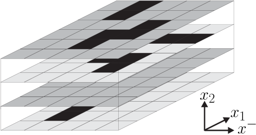
Figure 1: In the light cone limit of the nlc Hamiltonian, the ground state wave functional decouples the dynamics of the $(x^{-},x_{1})$- and $(x^{-},x_{2})$-planes from each other. Thus, one obtains many decoupled two-dimensional gauge theories. The planar structures (Wegner-Wilson loops) shown in black sketch vacuum fluctuations described by the ground state wave functional inside of the $(x^{-},x^{1})$-planes.

These are the reasons why Hamiltonian gluon dynamics on the light cone is considerably simplified compared with equal time Hamiltonian QCD. We have the following standard area law behavior for Wegner-Wilson loops $W$ in the $(x^{-},1)$ and $(x^{-},2)$ planes, namely for

$$W(0,\vec{0}_{\perp}\,;\,z{}^{-},\vec{d}_{\perp})=S_{-}(0,\vec{0}_{\perp}\,;\,z^{-},\vec{0}_{\perp})\,S_{\perp}(z^{-},\vec{0}_{\perp}\,;\,z^{-},\vec{d}_{\perp})S_{-}(z^{-},\vec{d}_{\perp}\,;\,0,\vec{d}_{\perp})\,S_{\perp}(0,\vec{d}_{\perp}\,;\,0,\vec{0}_{\perp})$$ (25)

expressible through the plaquettes

$$\left\langle\Psi_{0}\right|\frac{1}{2}\,\mathrm{Tr}\left[\,W(0,\vec{0}_{\perp}\,;\,z{}^{-},\vec{d}_{\perp})\,\right]\left|\Psi_{0}\right\rangle=\left(\left\langle\Psi_{0}\right|\frac{1}{2}\mathrm{Tr}\left[\,U_{-k}\,\right]\left|\Psi_{0}\right\rangle\right)^{d_{\perp}\,|z{}^{-}|}\;.$$ (26)

The physical area $\mathrm{A}$ of the Wegner-Wilson loop is given by $\mathrm{A}=d_{\perp}\,|z{}^{-}|\,a_{\perp}\,a_{-}$. Factorization is also true for expectation values of the product of two Wegner-Wilson loops which do not overlap. Single plaquette expectation values with respect to the ground state wave functional are given by

$$f_{1k} \equiv \left\langle\Psi_{0}\right|\frac{1}{2}\mathrm{Tr}\left[\,U_{-k}\,\right]\left|\Psi_{0}\right\rangle=\frac{I_{2}(4\,\rho_{0})}{I_{1}(4\,\rho_{0})}+\mathcal{O}(\delta_{0}^{2})\in[-1,1]$$

$$f_{2k} \equiv \left\langle\Psi_{0}\right|\left(\frac{1}{2}\mathrm{Tr}\left[\,U_{-k}\,\right]\right)^{2}\left|\Psi_{0}\right\rangle=\frac{I_{2}(4\,\rho_{0})}{4\,\rho_{0}\,I_{1}(4\,\rho_{0})}+\frac{I_{3}(4\,\rho_{0})}{I_{1}(4\,\rho_{0})}+\mathcal{O}(\delta_{0}^{2})\in[0,1]\,,$$ (27)

taking into account that higher powers of the same plaquette do not factorize. Here, $I_{n}$ denote the modified Bessel functions of the first kind. The very same relations hold for the purely transversal plaquette expectation values with $\rho_{0}$ substituted by $\delta_{0}$. By using Eq. (26) and Eq. (27), one can analytically evaluate all the gluonic matrix elements we need for our calculation. One can estimate the physical value of the transversal lattice spacing by identifying the rate of the exponential fall-off of a purely transversal Wegner-Wilson loop with the dimensionless string tension. For example, one obtains a transversal lattice spacing of $a_{\perp}\approx 0.65\,\mathrm{fm}$ at $\lambda=10$. This corresponds to a momentum scale of $Q^{2}\approx 1\,\mathrm{GeV}^{2}$ which is the typical input scale for phenomenological parameterizations of parton distribution functions.

IV Modeling a color dipole

The near-light-cone Hamiltonian in Eq. (16) contains only gluon fields, therefore we cannot derive hadronic wave functions from this Hamiltonian. We have to make a model for the hadron taking into account the gluon structure as exactly as possible while treating the quarks only schematically. Our model consists of a dipole state with a fixed longitudinal center of mass momentum $p_{-}$ localized in transversal configuration space at a fixed center of mass position $\vec{b}_{\perp}=\vec{0}$ while the quark and antiquark positions are fixed at $\pm\vec{d}_{\perp}/2$, i.e. they are separated by the vector $\vec{d}_{\perp}$ and connected by a Schwinger string along some path $\mathcal{C}_{\perp}$ in the transversal plane specifying the dipole in transversal configuration space and longitudinal momentum space

$$\left|d(p_{-}\,;\,-\vec{d}_{\perp}/2,\mathcal{C}_{\perp},\vec{d}_{\perp}/2)\right\rangle\;.$$ (28)

For simplicity, we consider scalar QCD with a scalar matter field. The scalar quark fields can be expanded in terms of creation and annihilation operators

$$\Phi(x) = \Phi_{+}(x)+\Phi_{-}(x)\,,$$ (29)

$$\Phi_{+}(x)=\int d\tilde{k}\,a(k)\,e^{-\mathrm{i}k\,x}~{}~{},~{}~{}\Phi_{-}(x) = \int d\tilde{k}\,b^{\dagger}(k)\,e^{+\mathrm{i}k\,x}~{}~{},~{}~{}d\tilde{k}=\frac{d^{4}k}{(2\pi)^{4}}\,2\pi\delta^{(4)}(k^{2}-m^{2})\,.$$

Here, $\Phi_{+}(x)$ denotes the positive frequency part of the scalar field and $\Phi_{-}(x)$ represents the negative frequency part. The operators $a(k),a^{\dagger}(k)$ refer to the quark annihilation/creation operators whereas $b(k),b^{\dagger}(k)$ refer to the antiquark annihilation/creation operators. $m^{2}$ denotes the quark/antiquark mass squared.

In order to construct such a dipole state, we start with a dipole state which is localized also in longitudinal configuration space. Then the dipole state consists of a quark at longitudinal position $x^{-}$ and at transversal position $-\vec{d}_{\perp}/2$ and of an antiquark at the same $x^{-}$ and at transversal position $\vec{d}_{\perp}/2$ connected by a Schwinger string along the path $\mathcal{C}_{\perp}$ in the transversal plane in order to achieve gauge invariance. The transversal path $\mathcal{C}_{\perp}$ of $n$ steps is parameterized by the intermediate transversal positions $\vec{y}_{\perp}[j]$ ($j=1,n-1$) of the links passed by the path

$$\mathcal{C}_{\perp}:-\vec{d}_{\perp}/2\to\vec{y}_{\perp}[1]\to\vec{y}_{\perp}[2]\to\ldots\to\vec{y}_{\perp}[n-1]\to\vec{d}_{\perp}/2\,.$$ (30)

The entire dipole state localized in full configuration space is created by some operator $\chi^{\dagger}$ acting on the vacuum state

$$\left|\Omega\right\rangle=\left|\Phi_{0}\right\rangle\otimes\left|\Psi_{0}\right\rangle$$ (31)

of the entire Hilbert space including gauge fields and (scalar) quarks. The vacuum state $\left|\Phi_{0}\right\rangle$ of the (heavy) quark sector is assumed to be the Fock vacuum. The vacuum state of the gauge fields, however, is given by Eq. (21) and therefore of non-perturbative nature. The operator $\chi^{\dagger}$ has the form

$$\chi^{\dagger}\,\left|\Omega\right\rangle\Phi_{+}^{\dagger}(x^{-},-\vec{d}_{\perp}/2)\,S_{q\,\bar{q}}^{\mathcal{C}_{\perp}}(x^{-},-\vec{d}_{\perp}/2\,;\,x^{-},\vec{d}_{\perp}/2)[\{y_{j}^{-}\}]\,\Phi_{-\,}(x^{-},\vec{d}_{\perp}/2)\,\left|\Omega\right\rangle\,,$$ (32)

where the parallel transporter $S_{q\,\bar{q}}^{\mathcal{C}_{\perp}}$ represents the path ordered ($\mathcal{P}$-ordered) product of $n$ transversal link operators along the path $\mathcal{C}_{\perp}$ in the transversal plane.

In addition, we have allowed in Eq. (32) for different longitudinal positions of the transversal links as motivated below and have inserted longitudinal Schwinger string bits connecting the (otherwise adjacent) transversal links in order to retain gauge invariance

$$S_{q\,\bar{q}}^{\mathrm{C}_{\perp}}(x^{-},-\vec{d}_{\perp}/2\,;\,x^{-},\vec{d}_{\perp}/2)[\{y_{j}^{-}\}]\equiv S_{-}(x^{-},-\vec{d}_{\perp}/2;y_{1}^{-},-\vec{d}_{\perp}/2)\,S_{\perp}(y_{1}^{-},-\vec{d}_{\perp}/2\,;\,y_{1}^{-},\vec{y}_{\perp}[1])$$

$$\,\left[\mathcal{P}\prod\limits_{j=1}^{n-1}S_{-}(y_{j}^{-},\vec{y}_{\perp}[j];\,y_{j+1}^{-},\vec{y}_{\perp}[j])S_{\perp}(y_{j+1}^{-},\vec{y}_{\perp}[j]\,;\,y_{j+1}^{-},\vec{y}_{\perp}[j+1])\right]\,S_{-}(y_{n}^{-},\vec{d}_{\perp}/2\,;\,x^{-},\vec{d}_{\perp}/2)\,.$$

Here, $\vec{y}_{\perp}[n]=\vec{d}_{\perp}/2$. The argument in round brackets of $S_{q\,\bar{q}}^{\mathcal{C}_{\perp}}$ represents the starting and the end point of the wiggly string, whereas the argument in square brackets represents the set of longitudinal coordinates of the intermediate transversal links. A typical string configuration is graphically represented in Fig. 2 assuming a lattice structure. Each of the link operators represents a string bit of the entire string.

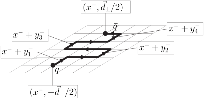
Figure 2: Graphical representation of the dipole state on the lattice. The black dots represent the quark and the antiquark. The transversal links are allowed to move freely along the longitudinal direction. For simplification only transversal links in one direction are shown. The coordinates $y_{j}^{-}$ denote the displacement of the link $j$ along the longitudinal direction with respect to the longitudinal position of the quark and antiquark.

The transversal part of the transporter between the quark and the antiquark along the vector $\vec{d}$ with minimal length (in purely transversal direction) represents the ground state of the nlc Hamiltonian in the strong coupling limit. In this limit, the nlc Hamiltonian is dominated by the chromo-electric field operators and the energy of the dipole state scales with the transversal length $|{\vec{d}}|$ of the gluonic string. Because of the Lorentz boost in the longitudinal direction accompanied by the transition from lab frame coordinates to nlc coordinates, the transverse electric field strength operators appear in the near-light-cone Hamiltonian with a weight larger by a factor $1/\tilde{\eta}^{2}$ compared to the longitudinal field strengths (c.f. Eq. (16)). Therefore every string with a fixed number of transversal links practically has the same energy regardless of the number of links in $x^{-}$-direction in the light cone limit $\tilde{\eta}\to 0$. This implies that the string should be defined having any number of longitudinal links.

The aim of our calculation is to calculate the gluon structure function for a color dipole with string configurations deformed in this manner, however with fixed momentum. We have to construct from the localized dipole in configuration space a fast moving momentum eigenstate with total longitudinal momentum $p_{-}$ for which we can determine the momenta of gluons. For this purpose we perform an integration over all translations of this state over the entire coordinate range multiplied with the appropriate momentum eigenfunctions $e^{-\mathrm{i}\,p_{-}\,x^{-}}$. Finally, weighting will be performed with the vacuum wave functional squared. Since none of the link configurations is preferable from the energetic point of view, we integrate over all possible link configurations and assign to each configuration a probability amplitude $\Psi(\{y_{j}^{-}\})$. We model $\Psi(\{y_{j}^{-}\})$ by the product of momentum eigenfunctions of each link integrated over all possible link momenta. Due to the projection of the entire dipole state onto total momentum $p_{-}$, the sum of its constituent momenta is restricted (c.f. Eq. (14)), i.e.

$$\Psi(\{y_{j}^{-}\})=\int\limits_{0}^{\infty}\left(\prod\limits_{j=1}^{n}dl_{-}^{j}\right)\,e^{-\mathrm{i}\,\sum\limits_{j=1}^{n}l_{-}^{j}\,y_{j}^{-}}\,\Theta\left(p_{-}-\sum_{j=1}^{n}l_{-}^{j}\right)\;.$$ (34)

Hence, the final dipole state is given by

$$\left|d(p_{-}\,;\,-\vec{d}_{\bot}/2,\mathrm{C}_{\perp},\vec{d}_{\perp}/2)\right\rangle=\frac{1}{\sqrt{N}}\int\left(\prod\limits_{j=1}^{n}dl_{-}^{j}dy_{j}^{-}\right)\,e^{-\mathrm{i}\,\sum\limits_{j=1}^{n}l_{-}^{j}\,y_{j}^{-}}\,\Theta\left(p_{-}-\sum_{j=1}^{n}l_{-}^{j}\right)$$

$$\times\int dx^{-}\,e^{-\mathrm{i}\,p_{-}\,x^{-}}\,\Phi_{+}^{\dagger}(x^{-},-\vec{d}_{\perp}/2)\,S_{q\,\bar{q}}^{\mathrm{C}_{\perp}}(x^{-},-\vec{d}_{\perp}/2\,;\,x^{-},\vec{d}_{\perp}/2)[\{x^{-}+y_{j}^{-}\}]\,\Phi_{-}(x^{-},\vec{d}_{\perp}/2)\,\left|\Omega\right\rangle\,.$$

The appropriate normalization of the dipole state is guaranteed by division with a suitable normalization factor $\sqrt{N}$. This dipole state represents the starting point for our investigation of its gluon structure.

Matrix elements between two dipole states can be computed by contracting the scalar operators $\Phi_{\pm}$ yielding the Feynman propagator $\Delta_{F}(x,y|A)$. We find for the Feynman propagator of the interacting scalar theory in the eikonal approximation (quark/antiquark have large $p_{+}$ momenta)

$$\Delta_{F}(x,y|A) = \frac{p_{-}}{m^{2}}\,\left[\Theta(x^{-}-y^{-})\,e^{-\mathrm{i}\,p_{-}\,(x^{-}-y^{-})}\,+\Theta(y^{-}-x^{-})\,e^{-\mathrm{i}\,p_{-}\,(y^{-}-x^{-})}\right]$$ (36)

$$\times S_{-}(x^{-},\vec{x}_{\perp}~{};~{}y^{-},\vec{x}_{\perp})\,\delta^{(2)}(\vec{x}_{\perp}-\vec{y}_{\perp})\,\delta(x^{+}-y^{+})\,.$$

At high $p_{+}$-momentum, the quark and antiquark in the color dipole move on straight line classical trajectories and pick up non-abelian phase factors along their paths. Instead of the usual time ordering, we have an ordering along the longitudinal spatial coordinate. Thus, by evaluating matrix elements between two dipole states, additional straight line Schwinger strings appear along the longitudinal direction connecting the wiggly Schwinger strings from the incoming and outgoing dipole states. To evaluate the expectation value of the point split operator $G$ (given in Eq. (11)) between two dipole states with fixed string configurations the following expression can be reduced to a purely gluonic matrix element

$$\left\langle\Omega\right|\Big{(}\Phi_{+}^{\dagger}(x^{\prime}{}^{-},\vec{x}_{\perp}{}^{\prime})\,S_{q\bar{q}}^{\mathrm{C}_{\perp}^{\prime}}\big{(}x^{\prime}{}^{-},\,\vec{x}_{\perp}{}^{\prime}\,;\,x^{\prime}{}^{-},\,\vec{x}_{\perp}{}^{\prime}+\vec{d}_{\perp}{}^{\prime}\big{)}[\{y_{j}^{\prime}{}^{-}\}]\,\Phi_{-}(x^{\prime}{}^{-},\vec{x}_{\perp}{}^{\prime}+\vec{d}_{\perp}{}^{\prime})\Big{)}^{\dagger}$$ (37)

$$~{}~{}~{}~{}~{}~{}~{}~{}\times G\,\Big{(}\Phi_{+}^{\dagger}(x^{-},\vec{x}_{\perp})\,S_{q\bar{q}}^{\mathrm{C}_{\perp}}\big{(}x^{-},\vec{x}_{\perp}\,;\,x^{-},\vec{x}_{\perp}+\vec{d}_{\perp}\big{)}[\{y_{j}^{-}\}]\,\Phi_{-}(x^{-},\vec{x}_{\perp}+\vec{d}_{\perp})\Big{)}\left|\Omega\right\rangle$$

$$= \left\langle\Psi_{0}\right|\mathrm{Tr}\Big{[}S_{-}(x^{-},\vec{x}_{\perp}+\vec{d}_{\perp}\,;\,x^{\prime}{}^{-};\vec{x}_{\perp}+\vec{d}_{\perp})\,S_{q\bar{q}}^{\mathrm{C}_{\perp}^{\prime}}\big{(}x^{\prime}{}^{-},\vec{x}_{\perp}\,;x^{\prime}{}^{-},\vec{x}_{\perp}+\vec{d}_{\perp}\,\big{)}[\{y_{j}^{\prime}{}^{-}\}]^{\dagger}$$

$$~{}~{}~{}~{}~{}~{}~{}~{}~{}~{}~{}~{}\times S_{-}(x^{\prime}{}^{-},\vec{x}_{\perp}\,;\,x^{-};\vec{x}_{\perp})\,G\,S_{q\bar{q}}^{\mathrm{C}_{\perp}}\big{(}x^{-},\vec{x}_{\perp}\,;\,x^{-},\vec{x}_{\perp}+\vec{d}_{\perp}\big{)}[\{y_{j}^{-}\}]\Big{]}\left|\Psi_{0}\right\rangle$$

$$~{}~{}~{}~{}~{}\times\frac{p_{-}^{q}\,p_{-}^{\bar{q}}}{m^{4}}\,e^{\mathrm{i}(p_{-}^{q}+p_{-}^{\bar{q}})(x^{-}-x^{\prime}{}^{-})}\,\delta^{(2)}(\vec{x}_{\perp}-\vec{x}_{\perp}{}^{\prime})\,\delta^{(2)}(\vec{d}_{\perp}-\vec{d}_{\perp}{}^{\prime})$$

to be obtained by averaging over the vacuum wave functional squared. The transversal chromo-electric field operators appearing in Eq. (11) do not commute with the transversal link operators appearing in the definition of the dipole operator. Therefore, one has to take care of the right arrangement of the operators. The string $S_{q\bar{q}}^{\mathcal{C}_{\perp}^{\prime}\,\dagger}(x^{\prime\,-})$ arising from the dipole at $x^{\prime}{}^{-}$ must appear to the left of the operator $G(z^{-},\vec{z}_{\perp}\,;\,z^{-}{}^{\prime},\vec{z}_{\perp})$ and correspondingly the string $S_{q\bar{q}}^{\mathcal{C}_{\perp}}(x^{-})$ to the right of $G(z^{-},\vec{z}_{\perp}\,;\,z^{-}{}^{\prime},\vec{z}_{\perp})$ in the matrix element. The resulting Eq. (37) allows to express the expectation value of the momentum density operator between dipole states by the gluonic vacuum average of the trace over a non-rectangular Wegner-Wilson loop whose edges are given by the transversal parallel transporters $S_{q\bar{q}}^{\mathcal{C}_{\perp}}$, $S_{q\bar{q}}^{\mathcal{C}_{\perp}^{\prime}\,\dagger}$ and the longitudinal straight line Schwinger strings connecting the two dipole states. Such a Wilson loop is shown in Fig. 3, for simplification with only one transverse dimension and the $x^{-}$-direction. The full curves represent the strings which connect the quark and antiquark in each of the dipole states. The dotted strings arise due to the elimination of the quark/antiquark operators in the eikonal approximation of the quark propagator. The blue curve corresponds to the point split operator $G$. Note, that in general the wiggly string can extend into both transverse directions and the $x^{-}$-direction.

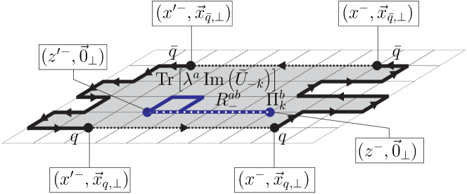
Figure 3: Graphical representation of the generalized Wegner-Wilson loop generated by the two color dipole states with a quark $q$ and an antiquark $\bar{q}$ connected by n-links in transversal direction. For simplification only transversal links in one direction are shown. The dash-dotted insertion in the so-formed Wegner-Wilson loop represents the gluonic two-point operator with a lattice electric field operator at longitudinal coordinate $z^{-}$ and a lattice magnetic field operator at longitudinal coordinate $z^{\prime}{}^{-}$.

After the quark fields are eliminated, the $x^{-}$ integration in Eq. (IV) can be performed for the incoming and outgoing dipole state and yields together with the quark and antiquark momenta from Eq. (37) a delta distribution setting the sum of transversal link momenta equal to the total string momentum $p_{-}^{S}$

$$\delta\left(p_{-}^{S}-\sum_{j=1}^{n}l_{-}^{j}\right)~{}~{},~{}~{}p_{-}^{S}=p_{-}-p_{-}^{q}-p_{-}^{\bar{q}}\,.$$ (38)

In order to compute the normalization of the dipole state, one simply has to substitute the point split operator $G$ in Eq. (37) by the unit operator.

V Near-light-cone gluon correlation function on the
lattice

We come now to the practical evaluation of the lattice counterpart of the gluon distribution function. On the lattice, a direct simulation of the average gluon momentum fraction becomes subtle. Being the lattice generator of longitudinal translations, the longitudinal momentum operator induces translations by any multiple of the lattice unit. We discriminate between longitudinal lattice momenta and eigenvalues of the longitudinal lattice momentum operator in the following. Similar to the dispersion relation for fermions on the lattice, one has for each positive valued eigenvalue in the spectrum of the longitudinal lattice momentum operator two possible lattice momenta corresponding to this eigenvalue. Even worse, the largest possible lattice momentum corresponds to an eigenvalue of the longitudinal momentum operator close to zero, far away from its maximal possible value. Hence, by choosing the hadron to have the maximal lattice momentum, one finds gluon momentum fractions which do not add up to unity (neglecting quark momenta).

We discuss first how the problem arises and second how to circumvent it. We start discretizing the point split operator of the nlc correlation function Eq. (11) :

$$G(z^{-},\vec{z}_{\perp}~{};~{}z^{\prime}{}^{-},\vec{z}_{\perp})$$

$$= \frac{1}{4}\,\sum\limits_{k}\Big{(}2\,\Pi_{k}^{a}(z^{-},\vec{z}_{\perp})\,S_{ab}^{A}(z^{-},\vec{z}_{\perp}~{};~{}z^{\prime}{}^{-},\vec{z}_{\perp})\,\mathrm{Tr}\left[\,\frac{\sigma^{b}}{2}\,\mathrm{Im}\Big{(}\,\overline{U}_{-k}(z^{\prime}{}^{-},\vec{z}_{\perp})\,\Big{)}\,\right]$$

$$~{}~{}~{}~{}~{}~{}~{}~{}~{}~{}~{}+2\,\Pi_{k}^{a}(z^{\prime}{}^{-},\vec{z}_{\perp})\,S_{ab}^{A}(z^{\prime}{}^{-},\vec{z}_{\perp},z^{-},\vec{z}_{\perp})\,\mathrm{Tr}\left[\,\frac{\sigma^{b}}{2}\,\mathrm{Im}\Big{(}\,\overline{U}_{-k}(z^{-},\vec{z}_{\perp})\,\Big{)}\,\right]+h.c.\Big{)}\,.$$

The field strength $F_{-k}^{a}$ in lattice form is expressed here in such a way that Eq. (11) follows in the naive continuum limit. Here, $\overline{U}_{-k}(\vec{x})$ is an average over the ”forward” plaquette $U_{-k}^{\rm forw}(\vec{x})$ right of $x^{-}$ and of the ”backward” plaquette $U_{-k}^{\rm backw}(\vec{x})$ left of $x^{-}$, both $-k$ plaquettes beginning in $x$ and adjacent to the transversal link $U_{k}(\vec{x})$ :

$$\overline{U}_{-k}(\vec{x})\equiv\frac{1}{2}\left(U_{-k}^{\rm forw}(\vec{x})+U_{-k}^{\rm backw}(\vec{x})\right)$$ (40)

with

$$U_{-k}^{\rm forw}(\vec{x})\equiv U_{-}(\vec{x})U_{k}(\vec{x}+\widehat{e}_{-})U_{-}^{\dagger}(\vec{x}+\widehat{e}_{k})U_{k}^{\dagger}(\vec{x})$$ (41)

and

$$U_{-k}^{\rm backw}(\vec{x})\equiv U_{k}(\vec{x})U_{-}^{\dagger}(\vec{x}+\widehat{e}_{k}-\widehat{e}_{-})U_{k}^{\dagger}(\vec{x}-\widehat{e}_{-})U_{-}(\vec{x}-\widehat{e}_{-})\;.$$ (42)

Note, that the orientations of the forward and backward plaquettes are the same such that the projection of the traceless antihermitean part $\mathrm{Im}\,\overline{U}_{-k}$ onto $\sigma^{a}/2$ becomes proportional to $F_{-k}^{a}(\vec{x})$ in the continuum limit.

For $z^{\prime}{}^{-}=z^{-}$, the point split operator reduces to the dimensionless nlc momentum density operator (c.f. Eq. (9)) with $\vec{z}=(z^{-},\vec{z}_{\perp})$, the lattice form of which is

$$\mathcal{P}_{-}(\vec{z}) = \sum\limits_{k}\frac{1}{2}\Big{(}2\,\Pi_{k}^{a}(\vec{z})\,\mathrm{Tr}\left[\,\frac{\sigma^{a}}{2}\,\mathrm{Im}\Big{(}\,\overline{U}_{-k}(\vec{z})\,\Big{)}\,\right]$$ (43)

$$~{}~{}~{}~{}~{}~{}~{}~{}~{}~{}~{}~{}~{}~{}+2\,\mathrm{Tr}\left[\,\frac{\sigma^{a}}{2}\,\mathrm{Im}\Big{(}\,\overline{U}_{-k}(\vec{z})\,\Big{)}\,\right]\Pi_{k}^{a}(\vec{z})\Big{)}\,,$$

which becomes the total longitudinal momentum operator $P_{-}$ when summed over the entire lattice. The variational ground state wave functional ansatz Eq. (21) is an exact eigen state of the longitudinal momentum operator with eigen value equal to zero for $\delta_{0}=0$, i.e.

$$\sum_{\vec{z}}\mathcal{P}_{-}(\vec{z})\,\left|\Psi_{0}\right\rangle=0+\mathcal{O}(\delta_{0})\,.$$ (44)

To find the spectrum of the total longitudinal momentum operator, one has to know how it acts on link operators. The commutator of the total momentum operator $P_{-}=\sum_{\vec{z}}\mathcal{P}_{-}(\vec{z})$ with a transversal link $U_{j}(\vec{y})$ being part of the gluonic string forming the hadron state gives (c.f. Eq. (19))

$$\left[\sum_{\vec{z}}\mathcal{P}_{-}(\vec{z}),U_{j}(\vec{y})\right] = \frac{1}{4\,\mathrm{i}}\left(U_{-}(\vec{y})\,U_{j}(\vec{y}+\vec{e}_{-})\,U^{\dagger}_{-}(\vec{y}+\vec{e}_{j})-U_{-j}^{{\rm forw}\,\dagger}(\vec{y})\,U_{j}(\vec{y})+U_{-j}^{\rm backw}(\vec{y})\,U_{j}(\vec{y})\right.$$ (45)

$$~{}~{}~{}~{}~{}~{}~{}~{}~{}~{}\left.-U_{-}^{\dagger}(\vec{y}-\vec{e}_{-})\,U_{j}(\vec{y}-\vec{e}_{-})\,U_{-}(\vec{y}+\vec{e}_{j}-\vec{e}_{-})\right)$$

$$= \frac{1}{2\,\mathrm{i}}\left(U_{-}(\vec{y})\,U_{j}(\vec{y}+\vec{e}_{-})\,U^{\dagger}_{-}(\vec{y}+\vec{e}_{j})\right.$$

$$\left.~{}~{}~{}~{}~{}-U_{-}^{\dagger}(\vec{y}-\vec{e}_{-})\,U_{j}(\vec{y}-\vec{e}_{-})\,U_{-}(\vec{y}+\vec{e}_{j}-\vec{e}_{-})\right)+\mathcal{O}(a^{2})\,.$$

The first line of Eq. (45) (containing also “curled-up” plaquette insertions into the gluonic string) is exact and will be used in subsequent calculations. The exact commutator of $P_{-}$ with the link $U_{j}$ symbolized by the arrow has the following graphical representation

$$\left[P_{-},\mbox{ \begin{picture}(0.2,1.1)\put(0.05,0.1){\vector(0,1){1.0}} \put(-0.1,-0.4){\scriptsize$\vec{y}$ } \end{picture}}\right]=\frac{1}{4\,\mathrm{i}}\left(\mbox{ \begin{picture}(1.7,0.1)\put(0.0,0.1){\vector(1,0){1.0}} \put(1.0,0.1){\vector(0,1){1.0}} \put(1.0,1.1){\vector(-1,0){1.0}} \put(0.4,-0.6){\scriptsize$\vec{y}+\vec{e}_{-}$ } \end{picture}}-\mbox{ \begin{picture}(1.7,0.1)\put(0.0,0.1){\vector(0,1){1.0}} \put(0.0,1.1){\vector(1,0){1.0}} \put(1.0,1.1){\vector(0,-1){1.0}} \put(1.0,0.1){\vector(-1,0){0.8}} \put(0.2,0.1){\vector(0,1){1.0}} \put(0.2,1.1){\line(0,1){0.2}} \put(0.4,-0.6){\scriptsize$\vec{y}+\vec{e}_{-}$ } \end{picture}}+\mbox{ \begin{picture}(1.1,1.1)\put(1.0,0.1){\vector(0,1){1.0}} \put(1.0,1.1){\vector(-1,0){1.0}} \put(0.0,1.1){\vector(0,-1){1.0}} \put(0.0,0.1){\vector(1,0){0.8}} \put(0.8,0.1){\vector(0,1){1.0}} \put(0.8,1.1){\line(0,1){0.2}} \put(-0.6,-0.6){\scriptsize$\vec{y}-\vec{e}_{-}$ } \end{picture}}-\mbox{ \begin{picture}(1.1,1.1)\put(1.0,0.1){\vector(-1,0){1.0}} \put(0.0,0.1){\vector(0,1){1.0}} \put(0.0,1.1){\vector(1,0){1.0}} \put(-0.6,-0.6){\scriptsize$\vec{y}-\vec{e}_{-}$ } \end{picture}}\right)\,.$$ (46)

In the second line of Eq. (45), we have expanded the result in powers of the lattice spacing up to quadratic corrections $\mathcal{O}(a^{2})$, where $a^{2}$ stands for $(a_{-}^{2},a_{-}\,a_{\perp},a_{\perp}^{2})$. Then the commutator of $P_{-}$ with the link $U_{j}$ corresponds to gauge invariant forward and backward translations along the longitudinal direction

$$\left[P_{-},\mbox{ \begin{picture}(0.2,1.1)\put(0.05,0.1){\vector(0,1){1.0}} \put(-0.1,-0.4){\scriptsize$\vec{y}$ } \end{picture}}\right]=\frac{1}{2\,\mathrm{i}}\left(\mbox{ \begin{picture}(1.7,0.1)\put(0.0,0.1){\vector(1,0){1.0}} \put(1.0,0.1){\vector(0,1){1.0}} \put(1.0,1.1){\vector(-1,0){1.0}} \put(0.4,-0.6){\scriptsize$\vec{y}+\vec{e}_{-}$ } \end{picture}}-\mbox{ \begin{picture}(1.1,1.1)\put(1.0,0.1){\vector(-1,0){1.0}} \put(0.0,0.1){\vector(0,1){1.0}} \put(0.0,1.1){\vector(1,0){1.0}} \put(-0.6,-0.6){\scriptsize$\vec{y}-\vec{e}_{-}$ } \end{picture}}\right)+\mathcal{O}(a^{2})\,,$$ (47)

i.e. leads to a discretized covariant first derivative of the link implemented in a symmetric way. The Heisenberg equation of motion for the transversal link on the lattice identifies the longitudinal momentum operator as the generator of longitudinal translations. In $A_{-}=0$ gauge, i.e. for $U_{-}=\mathds{1}$ the covariant derivative reduces to an ordinary discretized derivative.

Eigenstates of the longitudinal momentum operator can be found as sums of transverse links along the longitudinal direction modulated by appropriate phase factors up to corrections quadratic in the lattice constants $(a_{-},a_{\perp})$

$$\left[\sum_{\vec{z}}\mathcal{P}_{-}(\vec{z}),V_{j}(p_{-},\vec{y}_{\perp})\right]=\sin(p_{-})\,V_{j}(p_{-},\vec{y}_{\perp})+\mathcal{O}(a^{2})$$ (48)

with

$$V_{j}(p_{-},\vec{y}_{\perp})=\sum_{y^{-}}e^{-\mathrm{i}\,p_{-}\,y^{-}}\,U_{j}(y^{-},\vec{y}_{\perp})\,.$$ (49)

They arise from projecting transversal links localized in configuration space onto a definite longitudinal momentum $p_{-}$ and are not elements of $SU(2)$ because they are superpositions of link operators. The longitudinal lattice momenta must be an integer multiple $n$ of $2\,\pi/N_{-}$ with $n\leq 0\leq N_{-}/2-1$, since the longitudinal light cone momentum for an on shell particle is always positive (c.f. Eq. (14)). The momentum $p_{-}$ of the target is chosen as the largest momentum in order to have the maximum resolution in the gluon distribution function Pauli:1985ps ; Burkardt:2001jg

$$p_{-}=\frac{2\,\pi}{N_{-}}(N_{-}/2-1)\,.$$ (50)

Longitudinal lattice gluon momenta have the resolution

$$\frac{\Delta p_{-}^{g}}{p_{-}}=\frac{2}{N_{-}-2}\,.$$ (51)

In order to have a high resolution, the extension of the lattice in the longitudinal direction has to be very large.

Eqs. (48,50) imply that the largest lattice momentum $p_{-}$ yields an eigenvalue of the longitudinal momentum operator approximately equal to zero. Even though the gauge field is a bosonic degree of freedom, the eigen value $\sin(p_{-})$ of the discretized momentum operator looks ”fermionic” in the Brillouin zone $p_{-}\in[-\pi,\pi]$ of the longitudinal momentum, i.e. the map $p_{-}\to\sin(p_{-})$ is not injective.

In order to make it injective and monotonically increasing, we perform a similar but much simpler operation as for Kogut Susskind fermions, i.e. we block links on a sublattice with half of the lattice spacing along the longitudinal direction. Even sites on the fine lattice can be identified with lattice sites on the original lattice. Odd lattice sites on the fine lattice lie between two neighbouring original lattice sites. The physical extension $L_{\mathrm{phys}}$ and the physical momenta are kept fixed during the transition from the original to the fine lattice along the longitudinal direction

$$L_{\mathrm{phys}} = N_{-}\,a_{-}\,,$$

$$N_{-} = \frac{N_{-}^{f}}{2}\,,$$

$$a_{-} = 2\,a_{-}^{f}\,,$$

$$p_{-}^{f} = \frac{p_{-}}{2}\,.$$ (52)

We denote quantities on the fine sublattice by superscripts $f$. Using the fine lattice, we define a new momentum eigenstate $\widetilde{V}_{j}(p_{-},\vec{y}_{\perp})$ on the original lattice by a modulated sum over fine lattice links $U_{j}^{f}(y_{f}^{-},\vec{y}_{\perp})$

$$\widetilde{V}_{j}(p_{-},\vec{y}_{\perp})=\sum_{y^{-}_{f}}e^{-\mathrm{i}\,p_{-}^{f}\,y^{-}_{f}}\,\left.U_{j}^{f}(y_{f}^{-},\vec{y}_{\perp})\right|_{p_{-}^{f}=p_{-}/2}\,.$$ (53)

Thus, by keeping the physical momenta fixed, the allowed fine lattice momenta are given by one half of the original lattice momenta. Thereby we reduce the possible lattice momenta on the fine lattice by a factor of two and obtain a one-to-one correspondence between the lattice momenta and the eigenvalues on the fine lattice. The right hand side of Eq. (53) is obviously an eigenstate of the longitudinal momentum operator on the fine lattice albeit with eigenvalue $\sin(p_{-}^{f})$. However, Eq. (53) is not an eigenstate of the momentum operator on the original lattice, because the original momentum operator applied to the block averaged state does act solely on fine lattice links at even longitudinal fine lattice sites. Therefore, we have to introduce a block averaged longitudinal momentum density $\widetilde{\mathcal{P}}_{-}$ on the original lattice, acting on even and odd fine lattice sites. It is given by the following sum of fine momentum density operators $\mathcal{P}_{-}^{f}(z^{-}_{f},\vec{z}_{\perp})$ which are defined as in Eq. (43) with all operators on the fine lattice ($\Pi_{k}^{a}\rightarrow\Pi_{k}^{a\,f}$ and $U_{j}\rightarrow U_{j}^{f}$)

$$\widetilde{\mathcal{P}}_{-}(z^{-},\vec{z}_{\perp})=2\,\left(\frac{1}{2}\mathcal{P}_{-}^{f}(2\,z^{-}-1,\vec{z}_{\perp})+\mathcal{P}_{-}^{f}(2\,z^{-},\vec{z}_{\perp})+\frac{1}{2}\mathcal{P}_{-}^{f}(2\,z^{-}+1,\vec{z}_{\perp})\right)\,.$$ (54)

The factor two in front of the definition originates from converting the fine lattice operator into an operator on the coarse lattice, i.e. $P_{-}=2\,P_{-}^{f}$ similar to Eq. (52). The effective longitudinal momentum density on the original lattice Eq. (54) has contributions from even and odd sites on the fine lattice. Since we have symmetrized the operator with respect to the odd lattice sites on the fine lattice by using one half of the forward and one half of the backward contribution, $\widetilde{V}_{j}(p_{-},\vec{y}_{\perp})$ is an eigenstate of the effective longitudinal momentum operator on the original lattice with eigenvalue

$$\left[\widetilde{P}_{-},\widetilde{V}_{j}(p_{-},\vec{y}_{\perp})\right]=2\,\sin(p_{-}/2)\,\widetilde{V}_{j}(p_{-},\vec{y}_{\perp})+\mathcal{O}(a_{f}^{2})\,.$$ (55)

Now, the largest possible lattice momentum does also correspond to the largest possible eigenvalue of the momentum operator and the eigenvalues are monotonically increasing. The above expression Eq. (55) of the longitudinal momentum also appears in the dispersion relation for bosons $\omega=\sqrt{\sum_{i}(2\,\sin(p_{i}/2))^{2}+M^{2}}$ and defines a one-to-one mapping of the lattice momenta $p_{i}$ in the first Brillouin zone to the energy states. It represents an important stratification which allows to calculate momentum fractions. We define an effective correlation function $\widetilde{G}(z^{-},\vec{z}_{\perp}\,;\,z^{-}{}^{\prime},\vec{z}_{\perp})$ on the original lattice by averaging the correlation functions $G^{f}(z^{-}_{f},\vec{z}_{\perp}\,;\,z^{-}_{f}{}^{\prime},\vec{z}_{\perp})$ on the fine lattice Eq. (V)

$$\widetilde{G}(z^{-},\vec{z}_{\perp}\,;\,z^{-}{}^{\prime},\vec{z}_{\perp}) = 2\,\left(\frac{1}{2}G^{f}(2\,z^{-}-1,\vec{z}_{\perp}\,;\,2\,z^{-}{}^{\prime}-1,\vec{z}_{\perp})+G^{f}(2\,z^{-},\vec{z}_{\perp}\,;\,2\,z^{-}{}^{\prime},\vec{z}_{\perp})\right.$$ (56)

$$\left.+\frac{1}{2}G^{f}(2\,z^{-}+1,\vec{z}_{\perp}\,;\,2\,z^{-}{}^{\prime}+1,\vec{z}_{\perp})\right)\,.$$

This definition is in agreement with the longitudinal momentum density operator Eq. (54) on the coarse lattice for $z^{-}=z^{-}{}^{\prime}$. Finally, the lattice definition of the gluon distribution function is given by

$$g(p_{-}^{g})=\lim_{\eta\rightarrow 0}\,\frac{1}{\pi}\,\frac{1}{p_{-}^{g}}\sum_{z^{-},z^{\prime}{}^{-}}\,\sum_{\vec{z}_{\perp}}e^{-\mathrm{i}\,p_{-}^{g}(z^{-}-z^{\prime}{}^{-})}$$

$$\frac{\left\langle d(p_{-}\,;\,-\vec{d}_{\perp},\mathcal{C}_{\perp},\vec{d}_{\perp}/2)\right|\widetilde{G}(z^{-},\vec{z}_{\perp}~{};~{}z^{\prime}{}^{-},\vec{z}_{\perp})\left|d(p_{-}\,;\,-\vec{d}_{\perp},\mathcal{C}_{\perp},\vec{d}_{\perp}/2)\right\rangle_{c}}{\left\langle d(p_{-}\,;\,-\vec{d}_{\perp},\mathcal{C}_{\perp},\vec{d}_{\perp}/2)\right.\left|d(p_{-}\,;\,-\vec{d}_{\perp},\mathcal{C}_{\perp},\vec{d}_{\perp}/2)\right\rangle}\,.$$

In order not automatically to enforce Bjorken scaling, we prefer to express the gluon distribution function in terms of the gluon momentum $p_{-}^{g}$ instead of the momentum fraction $x_{B}$. Here, the gluonic component of the hadronic target state has to be defined by the block averaged momentum eigenstates given in Eq. (53).

On the lattice, the following orthogonality relation holds for positive gluon momenta

$$\frac{1}{N_{-}}\sum_{p_{-}^{g}=0}^{p_{-}}\mathrm{Re}\left[e^{-\mathrm{i}\,p_{-}^{g}\,z^{-}}\right]=\frac{1}{2}\delta_{z^{-},0}+\frac{1}{2\,N_{-}}\left(1-(-1)^{z^{-}}\right)=\frac{1}{2}\delta_{z^{-},0}+\mathcal{O}\left(\frac{1}{N_{-}}\right)\,.$$ (58)

Taking the real part in the orthogonality relation is sufficient since the point split operator is symmetric with respect to an interchange of $z^{-}$ and $z^{\prime}{}^{-}$. In addition to the continuum result $\delta_{z^{-},0}/2$, there is also a finite size contribution which vanishes like $1/N_{-}$. One finds the average gluon momentum $\langle p_{-}^{g}\rangle$

$$\left\langle p_{-}^{g}\right\rangle = \frac{2\,\pi}{N_{-}}\sum_{p_{-}^{g}=0}^{p_{-}}p_{-}^{g}\,g(p_{-}^{g})=\sum_{z^{-},\vec{z}_{\perp}}\left\langle\widetilde{\mathcal{P}}_{-}\right\rangle+\mathcal{O}\left(\frac{1}{N_{-}}\right)\,,$$

$$\sum_{z^{-},\vec{z}_{\perp}}\left\langle\widetilde{\mathcal{P}}_{-}\right\rangle = \sum_{z^{-}}\sum_{\vec{z}_{\perp}}\frac{\left\langle d(p_{-}\,;\,-\vec{d}_{\perp},\mathcal{C}_{\perp},\vec{d}_{\perp}/2)\right|\widetilde{\mathcal{P}}_{-}(z^{-},\vec{z}_{\perp})\left|d(p_{-}\,;\,-\vec{d}_{\perp},\mathcal{C}_{\perp},\vec{d}_{\perp}/2)\right\rangle_{c}}{\left\langle d(p_{-}\,;\,-\vec{d}_{\perp},\mathcal{C}_{\perp},\vec{d}_{\perp}/2)\right.\left|d(p_{-}\,;\,-\vec{d}_{\perp},\mathcal{C}_{\perp},\vec{d}_{\perp}/2)\right\rangle}\,$$

$$= \sum_{z^{-}}\sum_{\vec{z}_{\perp}}\frac{\left\langle d(p_{-}\,;\,-\vec{d}_{\perp},\mathcal{C}_{\perp},\vec{d}_{\perp}/2)\right|\widetilde{G}(z^{-},\vec{z}_{\perp}~{};~{}z^{-},\vec{z}_{\perp})\left|d(p_{-}\,;\,-\vec{d}_{\perp},\mathcal{C}_{\perp},\vec{d}_{\perp}/2)\right\rangle_{c}}{\left\langle d(p_{-}\,;\,-\vec{d}_{\perp},\mathcal{C}_{\perp},\vec{d}_{\perp}/2)\right.\left|d(p_{-}\,;\,-\vec{d}_{\perp},\mathcal{C}_{\perp},\vec{d}_{\perp}/2)\right\rangle}\,.$$

Here, the factor $2\,\pi/N_{-}$ is due to the discretized measure of the momentum integration. In the infinite volume limit, the leading contribution is of order $\mathcal{O}(1)$ due to the normalization of the dipole state.

VI Gluon structure function of a one-link dipole

We start with the computation of the gluon structure function for the one-link dipole. Later we will consider the gluon structure function of the more sophisticated multi-link dipole. For a computation we use the dipole state Eq. (IV) reduced to a single link. Since the pure glue Hamiltonian of Eq. (16) does not control quark dynamics we have to choose between two alternatives:

• let the quark and antiquark simply follow the gluon link to which they are attached to and fix the quark and antiquark momenta to the correspondent link momentum.

• impose the quark dynamics of the color dipole externally. Since the total hadron longitudinal momentum is given by the sum of the momenta of its constituents, the total gluon momentum is then fixed.

We follow the second alternative and take the mean gluon momentum from experiment. At the input scale $Q^{2}\approx\pi^{2}/a_{\perp}^{2}=1.5\,\mathrm{GeV}^{2}$ corresponding to $\lambda\approx 10$ (c.f. Sec. III), we use the MRST-parameterization Martin:2001es and assign a mean momentum fraction $p_{-}^{S}=0.38\,p_{-}$ to the string. The string momentum $p_{-}^{S}$ results from the difference of hadron momentum and quark and the antiquark momenta which is taken from experiment:

$$p_{-}^{S}=p_{-}-p_{-}^{q}-p_{-}^{\bar{q}}\,.$$ (60)

We ascribe this momentum $p_{-}^{S}$ to the complete string of gluon links. Its transverse size $\vec{d}_{\bot}$ now equals one of the lattice unit vector $\vec{e}_{j}$, where $j=1,2$ denote the transversal directions

$$\vec{d}_{\bot}=\vec{e}_{j}~{}~{},~{}~{}j=1,2\,.$$ (61)

According to Eq. (37), the norm of the one-link dipole is related to the matrix element of a Wegner-Wilson loop defined by the eikonal trajectories $S_{-}^{f},S_{-}^{f}{}^{\dagger}$ of the quark and antiquark (dotted lines) together with the strings (full lines) $S_{q\bar{q}}^{f\,\dagger}[x_{f}^{\prime}]$, $S_{q\bar{q}}^{f}[x_{f}^{-}]$ inside of the color dipole (c.f. Fig. 3). For a string consisting of a single link, we can not define the dipole state symmetrically with respect to the origin in transversal space. We choose without loss of generality the quark to be located at the origin in transversal space and extend the dipole along one of the positive transversal axes with the antiquark located at $\vec{e}_{j}$. Hence, the norm of the dipole state is given by

$$\left\langle d(p_{-}\,;\,\vec{0}_{\bot},\vec{d}_{\perp})\right|\left.d(p_{-}\,;\,\vec{0}_{\bot},\vec{d}_{\perp})\right\rangle=\frac{1}{N}\sum_{x_{f}^{-},x_{f}^{\prime}{}^{-}}e^{-\mathrm{i}\,p_{-}^{S}/2\,\left(x_{f}^{-}-x_{f}^{\prime}{}^{-}\right)}\left\langle\Psi_{0}\right|\mathrm{Tr}\Big{[}S_{-}^{f}(x_{f}^{-},\vec{d}_{\perp}\,;\,x_{f}^{\prime}{}^{-};\vec{d}_{\perp})\phantom{S_{q\bar{q}}^{f\,\dagger}\big{(}x_{f}^{\prime}{}^{-},\vec{0}_{\perp}\,\big{)}}$$ (62)

$$\times\,S_{q\bar{q}}^{f\,\dagger}\big{(}x_{f}^{\prime}{}^{-},\vec{0}_{\perp}\,;\,x_{f}^{\prime}{}^{-},\vec{d}_{\perp}\big{)}[x_{f}^{\prime}{}^{-}]\,S_{-}^{f}(x_{f}^{\prime}{}^{-},\vec{0}_{\perp}\,;\,x_{f}^{-},\vec{0}_{\perp})\,S_{q\bar{q}}^{f}\big{(}x_{f}^{-},\vec{0}_{\perp}\,;\,x_{f}^{-},\vec{d}_{\perp}\big{)}[x_{f}^{-}]\Big{]}\left|\Psi_{0}\right\rangle\,.$$

Here, we have suppressed the path index $\mathcal{C}_{\perp}$ in the state vectors. We absorb factors $2\,\pi$, volume factors due to the squared delta distributions and the factor $p_{-}^{q}\,p_{-}^{\bar{q}}/m^{4}$ appearing in Eq. (37) into the common normalization factor $N$. In the strong coupling approximation, this reduces to

$$\left\langle d(p_{-}\,;\,\vec{0}_{\bot},\vec{d}_{\perp})\right|\left.d(p_{-}\,;\,\vec{0}_{\bot},\vec{d}_{\perp})\right\rangle=\frac{1}{N}\,F_{1}(p_{-}^{S}),$$ (63)

where $F_{1}(p_{-}^{S})$ is given by

$$F_{1}(p_{-}^{S})=\sum_{x_{f}^{-},x_{f}^{-\,\prime}}e^{-\mathrm{i}\,p_{-}^{S}/2\big{(}x_{f}^{-}-x_{f}^{\prime}{}^{-}\big{)}}\Big{\langle}\frac{1}{2}\mathrm{Tr}\left[\,U_{-k}^{f}\,\right]\Big{\rangle}^{|x_{f}^{-}-x_{f}^{-\,\prime}|}\,.$$ (64)

In the gluon correlation function one has to take care of the arrangement of the operators. The transversal chromo-electric field operators in the point split operator Eq. (V) do not commute with the transversal link operators appearing in the definition of the dipole operator. As in the previous Sec. V, the string $S_{q\bar{q}}^{f\,\dagger}[x_{f}^{\prime\,-}]$ arising from the dipole at $x_{f}^{\prime}{}^{-}$ must appear to the left of the point split operator $\widetilde{G}(z^{-},\vec{z}_{\perp}\,;\,z^{-}{}^{\prime},\vec{z}_{\perp})$ and correspondingly the string $S_{q\bar{q}}^{f}[x_{f}^{-}]$ to the right of $\widetilde{G}(z^{-},\vec{z}_{\perp}\,;\,z^{-}{}^{\prime},\vec{z}_{\perp})$ (see Fig. 3). Then the forward matrix element of $\widetilde{G}(z^{-},\vec{z}_{\perp}\,;\,z^{-}{}^{\prime},\vec{z}_{\perp})$ is given by

$$\left\langle d(p_{-}\,;\,\vec{0}_{\bot},\vec{d}_{\perp})\right|\,\widetilde{G}(z^{-},\vec{z}_{\perp}\,;\,z^{-}{}^{\prime},\vec{z}_{\perp})\,\left|d(p_{-}\,;\,\vec{0}_{\bot},\vec{d}_{\perp}))\right\rangle=\frac{1}{N}\sum_{x_{f}^{-}\,,\,x_{f}^{\prime}{}^{-}}e^{-\mathrm{i}p_{-}^{S}/2\big{(}x_{f}^{-}-x_{f}^{\prime}{}^{-}\big{)}}$$ (65)

$$~{}~{}~{}~{}~{}~{}~{}~{}~{}~{}~{}~{}~{}~{}~{}\,\left\langle\Psi_{0}\right|\Big{[}S_{-}^{f}(x_{f}^{-},\vec{d}_{\perp}\,;\,x_{f}^{\prime}{}^{-};\vec{d}_{\perp})\,S_{q\bar{q}}^{f\,\dagger}\big{(}x_{f}^{\prime}{}^{-},\vec{0}_{\perp}\,;\,x_{f}^{\prime}{}^{-},\vec{d}_{\perp}\big{)}[x_{f}^{\prime}{}^{-}]\,S_{-}^{f}(x^{\prime}{}^{-},\vec{0}_{\perp}\,;\,x^{-},\vec{0}_{\perp})\Big{]}_{ab}$$

$$~{}~{}~{}~{}~{}~{}~{}~{}~{}~{}~{}~{}~{}~{}~{}~{}~{}~{}~{}~{}~{}~{}~{}~{}~{}~{}~{}~{}~{}\widetilde{G}(z^{-},\vec{z}_{\perp}\,;\,z^{-}{}^{\prime},\vec{z}_{\perp})\Big{[}S_{q\bar{q}}^{f}\big{(}x_{f}^{-},\vec{0}_{\perp}\,;\,x_{f}^{-},\vec{d}_{\perp}\big{)}[x_{f}^{-}]\Big{]}_{ba}\left|\Psi_{0}\right\rangle\,.$$

The square brackets denote matrix elements with color indices $ab$ and $ba$ respectively such that the expectation value is given by the trace over the product of the color dipole states $S^{\dagger}_{q\bar{q}}$ and $S_{q\bar{q}}^{f}$ with the effective point split operator $\widetilde{G}$ in between. The momentum correlation function Eq. (65) evaluates the cross product of electric and magnetic field strengths separated along the light cone, i.e. it determines the correlation of an electric field in the dipole with the corresponding magnetic field. In order to compute it, we arrange the operator $\widetilde{G}$ with $\left|\Psi_{0}\right\rangle$ (c.f. Eq. (21)) in a way such that $\widetilde{G}$ stands directly in front of the trivial ground state $\left|0\right\rangle$

$$\widetilde{G}\,S_{q\bar{q}}^{f}\,\left|\Psi_{0}\right\rangle=\left[\widetilde{G},S_{q\bar{q}}^{f}\right]\,\left|\Psi_{0}\right\rangle+S_{q\bar{q}}^{f}\,\left[\widetilde{G},\Psi_{0}\right]\,\left|0\right\rangle+S_{q\bar{q}}^{f}\,\Psi_{0}\,\widetilde{G}\,\left|0\right\rangle\,.$$ (66)

The trivial ground state is annihilated by this operator. The commutator of $\widetilde{G}$ with the ground state wave functional leaves the dipole operator intact and yields a vacuum transition which is subtracted when the connected matrix element is extracted. Therefore, the only remaining contribution comes from the commutator of $\widetilde{G}$ with the transversal link of the incoming dipole. It is given by

$$\left[G^{f}(z_{f}^{-},\vec{z}_{\perp}\,;\,z_{f}^{-\,\prime},\vec{z}_{\perp})\,,\,U_{j}^{f}(x_{f}^{-},\vec{x}_{\perp})\right]=$$ (67)

$$\phantom{+}\frac{1}{2}S_{-}^{f}(x_{f}^{-},\vec{x}_{\perp}\,;\,z_{f}^{-},\vec{x}_{\perp})\,\mathrm{Im}\Big{(}\,\bar{U}_{-j}^{f}(z_{f}^{-},\vec{x}_{\perp})\,\Big{)}\,S_{-}^{f}(z_{f}^{-},\vec{x}_{\perp}\,;\,x_{f}^{-},\vec{x}_{\perp})U_{j}^{f}(x^{-}_{f},\vec{x}_{\perp})\,\delta_{x_{f}^{-},z_{f}^{-\,\prime}}\,\delta_{\vec{x}_{\perp},\vec{z}_{\perp}}$$

$$+\,(z_{f}^{-}\leftrightarrow z_{f}^{-\,\prime})~{}.$$

Due to the interchange symmetry $z^{-}\leftrightarrow z^{\prime}{}^{-}$ of the commutator, only the $\cos$-part of the Fourier transformation survives:

$$\sum_{z^{-},z^{-}{}^{\prime}=-N_{-}/2}^{N_{-}/2-1}\,e^{-\mathrm{i}\,p_{-}^{g}(z^{-}-z^{\prime}{}^{-})}\left[\widetilde{G}(z^{-},\vec{z}_{\perp}\,;\,z^{-\,\prime},\vec{z}_{\perp})\,,\,U_{j}^{f}(x_{f}^{-}\vec{x}_{\perp})\right]$$ (68)

$$= \sum_{z^{-}=-N_{-}/2}^{N_{-}/2-1}2\,\cos\left(p_{-}^{g}\,z^{-}\right)\,S_{-}^{f}(x^{-},\vec{x}_{\perp}\,;\,x_{f}^{-}+2\,z^{-},\vec{x}_{\perp})\,\mathrm{Im}\Big{(}\,\bar{U}_{-j}^{f}(x_{f}^{-}+2\,z^{-},\vec{x}_{\perp})\,\Big{)}$$

$$~{}~{}~{}~{}~{}~{}~{}~{}~{}~{}~{}~{}~{}~{}~{}~{}~{}~{}~{}\times S_{-}^{f}(x_{f}^{-}+2\,z^{-},\vec{x}_{\perp}\,;\,x_{f}^{-},\vec{x}_{\perp})\,U_{j}^{f}(x_{f}^{-},\vec{x}_{\perp})\,\delta_{\vec{x}_{\perp},\vec{z}_{\perp}}\,.$$

The gluon distribution function Eq. (V) for a one-link dipole with total string momentum $p_{-}^{S}$ becomes

$$g_{1}(p_{-}^{g};p_{-}^{S}) = \frac{4}{\pi}\frac{1}{p_{-}^{g}}\sum_{z^{-}}\cos\left(p_{-}^{g}\,z^{-}\right)\frac{N_{-}}{F_{1}(p_{-}^{S})}\sum_{x_{f}^{-}}e^{\mathrm{i}\,p_{-}^{S}/2\,x_{f}^{-}}$$ (69)

$$\left\langle\Psi_{0}\right|\mathrm{Tr}\left[S_{-}^{f}(0,\vec{d}_{\perp}\,;\,x_{f}^{-},\vec{d}_{\perp})\,U_{j}^{f\,\dagger}(x_{f}^{-},\vec{0}_{\perp})\,S_{-}^{f}(x_{f}^{-},\vec{0}_{\perp}\,;\,2\,z^{-},\vec{0}_{\perp})\right.$$

$$~{}~{}~{}~{}~{}~{}\left.\times\mathrm{Im}\Big{(}\,\bar{U}_{-j}^{f}(2\,z^{-},\vec{0}_{\perp})\,\Big{)}\,S_{-}^{f}(2\,z^{-},\vec{0}_{\perp}\,;\,0,\vec{0}_{\perp})\,U_{j}^{f}(0,\vec{0}_{\perp})\right]\left|\Psi_{0}\right\rangle\,.$$

In $g_{1}(p_{-}^{g};p_{-}^{S})$ we indicate the total string momentum by the argument $p_{-}^{S}$ and the number of transversal links by the index $n=1$.

In the following, we discuss the evaluation of the matrix element in Eq. (69). The imaginary part of a $U_{-j}^{f}$ plaquette (field strength) located at longitudinal position $2\,z^{-}$ has to be correlated with a closed loop of links in the longitudinal transversal plane located between longitudinal positions $0$ and $x^{-}_{f}$ as visualized in Fig. 4.

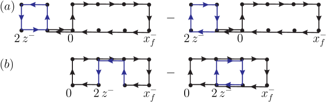
Figure 4: Visualization of the matrix element in Eq. (69). There are two different possible situations resulting in different expectation values of the operator, namely either the field strength lies outside of the Wegner-Wilson loop (a) or it lies inside (b). The difference in each of the two cases corresponds to the antihermitean part of the plaquette.

The field strength is connected with the edge of the Wegner-Wilson loop at longitudinal position $0$. We distinguish two cases depicted in Fig. 4 which can be fully evaluated in the strong coupling approximation:

• The plaquette $U_{-j}^{f}$ lies outside of the loop. The matrix element factorizes and vanishes due to $\mathrm{Tr}[\mathrm{Im}(U_{-j}^{f})]=0$.

• The plaquette lies inside the loop, the matrix element can be computed by tiling which yields the second line of Eq. (70).

One finally obtains for the gluon distribution function of a one-link dipole

$$g_{1}(p_{-}^{g},p_{-}^{S}) = \frac{4}{\pi}\frac{1}{p_{-}^{g}}\sum_{z^{-}}\cos\left(p_{-}^{g}\,z^{-}\right)\frac{N_{-}}{F_{1}(p_{-}^{S})}\sum_{x_{f}^{-}}\sin\left(\frac{p_{-}^{S}}{2}\,x_{f}^{-}\right)$$ (70)

$$\left(1-\Big{\langle}\Big{(}\frac{1}{2}\mathrm{Tr}\left[\,U_{-k}^{f}\,\right]\Big{)}^{2}\Big{\rangle}\right)\Big{\langle}\frac{1}{2}\mathrm{Tr}\left[\,U_{-k}^{f}\,\right]\Big{\rangle}^{|x_{f}^{-}|-1}$$

$$\times\left[\frac{1}{2}\Big{(}\Theta_{0}(2\,z^{-})\Theta(x_{f}^{-}-2\,z^{-})+\Theta(2\,z^{-})\Theta_{0}(x_{f}^{-}-2\,z^{-})\Big{)}\right.$$

$$~{}~{}~{}~{}~{}~{}~{}~{}\left.-\frac{1}{2}\Big{(}\Theta(-2\,z^{-})\Theta_{0}(2\,z^{-}-x_{f}^{-})+\Theta_{0}(-2\,z^{-})\Theta(2\,z^{-}-x_{f}^{-})\Big{)}\right]\,.$$

The two cases a) and b) are encoded in the $\Theta$-distributions $\Theta_{0}(x)$ and $\Theta(x)$ differing in the value they take at $x=0$, i.e.

$$\Theta(x)\equiv\left\{\begin{array}[]{lcl}1&,&x>0\\ 0&,&x\leq 0\end{array}\right.~{}~{},~{}~{}\Theta_{0}(x)\equiv\left\{\begin{array}[]{lcl}1&,&x\geq 0\\ 0&,&x<0\end{array}\right.~{}.$$ (71)

In the first line of Eq. (70), only the imaginary part $\sin(p_{-}^{S}/2\,x_{f}^{-})$ survives from the exponential $e^{-\mathrm{i}\,p_{-}^{S}/2\,x_{f}^{-}}$ due to the antisymmetry of the sum in $x^{-}_{f}$.

Let us now check the gluon momentum sum rule by evaluating the expectation value of the longitudinal momentum operator $\langle p_{-}^{g}\rangle=\sum_{z^{-},\vec{z}_{\perp}}\left\langle\widetilde{\mathcal{P}}_{-}(z^{-},\vec{z}_{\perp})\right\rangle$ as a function of the external string momentum $p_{-}^{S}$.

Figure 5: With crosses we show the expectation value of the longitudinal momentum operator $\widetilde{P}_{-}$ of a one-link dipole state as a function of $p_{-}=p_{-}^{S}$ on a $N_{-}=100$ lattice for $\lambda=10$ and $100$. We also show the expected eigenvalue $2\,\sin(p_{-}^{f}=p_{-}^{S}/2)$ of the longitudinal momentum operator without $\mathcal{O}(a^{2})$ corrections of a single-link color dipole state projected onto longitudinal momentum $p_{-}$.

In Fig. 5 we show the mean gluon momentum as a function of the lattice momentum $p_{-}^{S}$. The expectation value is obtained on a $N_{-}=100$ lattice for two different values of $\lambda$, i.e. $\lambda=10$ and $100$. In the region of small momenta $p_{-}^{S}$ one can recognise that the lattice discretisation is very accurate. Due to the introduction of the finer sublattice the mapping of the lattice momentum $p_{-}^{S}$ to the mean momentum $\langle p_{-}^{g}\rangle$ is unique. For comparison we also show the exact eigenvalue $2\sin(p_{-}^{S}/2)$ without order $\mathcal{O}(a^{2})$ corrections. The larger the lattice coupling constant, the more accurate becomes the mapping from lattice momenta to observed momenta.

The full gluon distribution function $p_{-}^{g}\,g_{1}(p_{-}^{g};p_{-}^{S})$ of a color dipole with one link in the transversal direction is shown in Fig. 6. It is computed on lattices with $N_{-}=20$, $30$, $50$, and $100$ sites in the longitudinal direction. The average gluon momentum $\langle p_{-}^{g}\rangle$ of the dipole state has been adjusted to the average gluon momentum $\langle p_{-}^{g}\rangle=0.38\,p_{-}$ of the MRST gluon distribution function at $Q^{2}=1.5\,\mathrm{GeV}^{2}$. So far, the simulated gluon distribution function on the lattice depends on the total hadron momentum. This is in contrast to Feynman scaling, where the gluon distribution function is only a function of the gluon momentum fraction $p_{-}^{g}/p_{-}$. For fixed $\lambda$, the hadronic lattice momentum $p_{-}=2\,\pi\,(N_{-}/2-1)/N_{-}$ is exclusively determined by the longitudinal lattice extension $N_{-}$. Independence of the gluon distribution function on the hadronic momentum would be equivalent to independence on the lattice extension.

Figure 6: Gluon distribution function $p_{-}^{g}\,g_{1}(p_{-}^{g}\,;\,p_{-}^{S}=0.38\,p_{-})$ of a color dipole with a single transversal link ($n=1$) in the transversal direction for different lattice sizes $N_{-}$. The distribution functions are computed with a lattice coupling $\lambda=4/g^{4}=10$ in the effective $SU(2)$ lattice Hamiltonian of Eq. (16). The average gluon momentum $\langle p_{-}^{g}\rangle=p_{-}^{S}$ of the dipole state has been adjusted to the average gluon momentum $\langle x_{B}\rangle\,p_{-}=0.38\,p_{-}$ of the MRST gluon distribution function at $Q^{2}=1.5\,\mathrm{GeV}^{2}$.

This figure demonstrates the effect of increasing the number of longitudinal lattice sites, i.e. approaching the infinite volume limit. Scaling for $\lambda=10$ seems to be obeyed for longitudinal lattice extensions larger than $N_{-}=50$. Realistic lattice simulations with an improved ground state wave functional need quite large longitudinal lattice sizes. The smearing of the distribution function is due to the gluon dynamics incorporated in the Wegner-Wilson loop expectation value. The area law behavior of the Wegner-Wilson loop yields a non-trivial gluon wave function which broadens the distribution.

If one varies the lattice gauge coupling $\lambda$, the single plaquette expectation values vary between $0$ and $1$ depending on the coupling constant $\lambda$. This has consequences for the width of the gluon distribution function $p_{-}^{g}\,g_{1}(p_{-}^{g};p_{-}^{S})$ as shown in Fig. 7. The larger $\lambda$, i.e. the smaller the QCD gauge coupling $g^{2}$, the stronger the peak in the one-link distribution function becomes.

Figure 7: Gluon distribution function $p_{-}^{g}\,g_{1}(p_{-}^{g};p_{-}^{S}=0.38\,p_{-})$ of a color dipole with a single transversal link ($n=1$) in the transversal direction at different lattice gauge couplings $\lambda$. The distribution functions have been computed on a lattice with $N_{-}=1000$ sites in the longitudinal direction. The average gluon momentum $\langle p_{-}^{g}\rangle$ of the dipole state has been adjusted to the average gluon momentum $\langle x_{B}\rangle\,p_{-}=0.38\,p_{-}$ of the MRST gluon distribution function at $Q^{2}=1.5\,\mathrm{GeV}^{2}$ .

In the extreme weak coupling limit $\lambda\rightarrow\infty$ the single plaquette expectation value approaches $1$. For finite coupling constants, the single plaquette expectation value is less than one. Hence, it suppresses large Wegner-Wilson loop extensions in Eq. (70):

$$W(0,\vec{0}_{\perp}\,;\,x_{f}{}^{-},\vec{d}_{\perp})=\Big{\langle}\frac{1}{2}\,\mathrm{Tr}\left[\,U_{-k}^{f}\,\right]\Big{\rangle}^{|x_{f}^{-}|}\,.$$ (72)

One can define a correlation length which represents the longitudinal distance at which the single plaquette expectation value reduces to one half of its original value

$$\Delta\xi=\log(\frac{1}{2})/\log\left(\Big{\langle}\frac{1}{2}\,\mathrm{Tr}\left[\,U_{-k}^{f}\,\right]\Big{\rangle}\right).$$ (73)

By using Eq. (23), Eq. (27) and Eq. (73), we can evaluate the correlation length directly as a function of $\lambda$. At $\lambda=10$, the correlation length is given by $\left.\Delta\xi\right|_{\lambda=10}=3.12$ and at $\lambda=50$ it is given by $\left.\Delta\xi\right|_{\lambda=50}=8.05$. Since the nlc gluon correlation function only has support when it lies inside the Wegner-Wilson loop, the correlation length $\Delta\xi$ gives an estimate for the width $\Delta p_{-}^{g}$ of the gluon momentum distribution,

$$\Delta p_{-}^{g}=\frac{1}{\Delta\xi}\,.$$ (74)

This implies that the width of the gluon momentum distribution at $\lambda=10$ is given by $\left.\Delta p_{-}^{g}\right|_{\lambda=10}=0.32$ and at $\lambda=50$ by $\left.\Delta p_{-}^{g}\right|_{\lambda=10}=0.13$ as seen in Fig. 7. In the extreme weak coupling limit, when the link reduces to a single gluon, the gluon distribution function is sharp, i.e. $g_{1}(p_{-}^{g};p_{-}^{S})=\delta(p_{-}^{g}-p_{-}^{S})$. Since the link momentum is fixed by the projection onto a definite momentum, also the gluon momentum is fixed in this limit and no variance is allowed. On the other hand, for smaller values of $\lambda=\frac{4}{g^{4}}$, i.e. for strong coupling the correlation length becomes smaller which implies that one has a broad momentum distribution peaked around $p_{-}^{S}$.

VII The gluon distribution function of a hadron

Up to now, we have considered the gluon distribution function of a color dipole consisting of a single transversal link. The one-link dipole gluon distribution is the basic building block from which the multiple link dipole gluon distribution function of a hadron can be constructed. We expand a hadronic state $\left|h(p_{-},\vec{0}_{\perp})\right\rangle$ in dipole components, i.e.

$$\left|h(p_{-},\vec{0}_{\perp})\right\rangle = \sum_{\mathcal{C},\vec{d}_{\perp}}\Psi_{h}(\mathcal{C},\vec{d}_{\perp})\left|d(p_{-}\,;\,-\vec{d}_{\perp}/2,\mathcal{C}_{\perp},\vec{d}_{\perp}/2)\right\rangle\,,$$

$$\Psi_{h}(\mathcal{C},\vec{d}_{\perp}) \equiv \Big{\langle}d(p_{-}\,;\,-\vec{d}_{\perp}/2,\mathcal{C}_{\perp},\vec{d}_{\perp}/2)\Big{.}\Big{|}h(p_{-},\vec{0}_{\perp})\Big{\rangle}\,.$$ (75)

The hadron has the same momentum $p_{-}$ and the same transversal cm coordinate $\vec{x}_{\perp}=0$ as the dipoles. The wave function $\Psi_{h}(\mathcal{C}_{\perp},\vec{d}_{\perp})$ represents the probability amplitude to find a dipole with a quark and an antiquark separated by the transversal distance $\vec{d}_{\perp}$ and connected by the path $\mathcal{C}_{\perp}$ in the hadron. Hence, the actual hadronic gluon distribution function arises from a superposition of multiple link configurations. The wiggly strings $S_{q\,\bar{q}}$ c.f. Eq. (IV) connecting the quark/antiquark are not restricted to lie along one of the coordinate axes (c.f. Fig. 2), but have a fixed number of transversal links as explained in Sec. IV. In order to project this state on angular momentum $J_{z}=0$, we rotate the hadron in the transversal plane by summing over randomly chosen curves $\mathcal{C}_{\perp}$ which can be constructed in the following way. A random walker starts at an initial time $t=0$ and trails a Schwinger string along its path through the transversal lattice. In each time step, the walker may hop with equal weight in one of the four transverse directions. The random walk ends if the number of hops corresponds to the number of allowed transversal links fixed by the energy constraint. The starting point of the random walker has to be chosen a posteriori in such a way that the center of mass of the generated dipole configuration is at the origin. The ensemble of possible random paths automatically obeys the desired rotational symmetry.

Since the energy of the strings with a given number of transversal links is the same for all the string configurations, we assume that the probabilities among the total number $\#$ of curves with n-links are equally distributed:

$$|\Psi_{h}(\mathcal{C},\vec{d})|^{2}=\frac{1}{\#}\,.$$ (76)

From the random walk follows that for n-links the hadron has an average radius squared $\vec{R}_{\perp}^{2}$ proportional to n: Hence, the area of the hadron scales with the number of links

$$\left\langle R_{\perp}^{2}\right\rangle=\frac{n\,a_{\perp}^{2}}{2}~{}.$$ (77)

Due to the strong coupling approximation non vanishing gluonic matrix elements need incoming and outgoing states to have the same curve connecting the quark and the antiquark:

$$\left\langle h(p_{-},\vec{0}_{\perp})\right|O\left|h(p_{-},\vec{0}_{\perp})\right\rangle=$$ (78)

$$\sum_{\mathcal{C},\vec{d}_{\perp}}\,\left|\Psi_{h}(\mathcal{C},\vec{d}_{\perp})\right|^{2}\,\left\langle d(p_{-}\,;\,-\vec{d}_{\perp}/2,\mathcal{C}_{\perp},\vec{d}_{\perp}/2)\right|O\left|d(p_{-}\,;\,-\vec{d}_{\perp}/2,\mathcal{C}_{\perp},\vec{d}_{\perp}/2)\right\rangle\,.$$

Because of the equal weight of all the dipole configurations with fixed transversal length n, the gluon distribution can be calculated from the distribution function $g_{n}$ of a string elongated along only one of the transversal axes (c.f. Fig. 2):

$$g_{h}(p_{-}^{g};p_{-}^{S})=g_{n}(p_{-}^{g};p_{-}^{S})\,.$$ (79)

Due to the sum rule (c.f. Eq. (V)) the expectation value of the gluon momentum inside the $n$-link dipole is fixed as $\langle p_{-}^{g}\rangle=p_{-}^{S}$. The computation of $g_{n}$ is done in analogy to the computation of the single-link gluon distribution. Because of the summation of the nlc correlation function over the entire transversal lattice, the chromo-electric field $\Pi_{k}^{a}$ in the operator defining the nlc correlation function, can act on each of the transversal links appearing in the connector $S_{q\bar{q}}$. In strong coupling the total loop factorizes, therefore the $n$-link distribution function is given by the product of a splitting function $P_{n\rightarrow n-1}$ multiplying the gluon distribution function with $n-1$ links . In this recursion relation (c.f. app. A) all possible intermediate momenta of the substring are summed over:

$$g_{n}\big{(}p_{-}^{g};p_{-}^{S}\big{)}=\frac{2\,\pi}{N_{-}}\sum_{p_{-}^{S}{}^{\prime}=0}^{p_{-}^{S}}g_{n-1}\big{(}p_{-}^{g};p_{-}^{S}{}^{\prime}\big{)}\,P_{n\rightarrow n-1}(p_{-}^{S},p_{-}^{S}{}^{\prime})\,.$$ (80)

The splitting function $P_{n\rightarrow n-1}(p_{-}^{S},p_{-}^{S}{}^{\prime})$ denotes the probability that a string with $n$ transversal links and total momentum $p_{-}^{S}$ splits into a string with $n-1$ transversal links and total momentum $p_{-}^{S}{}^{\prime}$. The form of the splitting function is of a kinematical and a dynamical origin which are both encoded in the functions $F_{m}(p_{-}^{S})$ for $m=n-1$ and $m=1$ due to the recursive representation:

$$P_{n\rightarrow n-1}(p_{-}^{S},p_{-}^{S}{}^{\prime})=\left(\frac{n}{n-1}\right)\times\frac{F_{n-1}\big{(}p_{-}^{S}{}^{\prime}\big{)}\,F_{1}\big{(}p_{-}^{S}-p_{-}^{S}{}^{\prime}\big{)}}{\frac{2\,\pi}{N_{-}}\sum_{p_{-}^{S}{}^{\prime\prime}=0}^{p_{-}^{S}}F_{n-1}\big{(}p_{-}^{S}{}^{\prime\prime}\big{)}\,F_{1}\big{(}p_{-}^{S}-p_{-}^{S}{}^{\prime\prime}\big{)}}\,.$$ (81)

The functions $F_{n-1}(p_{-}^{S})$ and $F_{1}(p_{-}^{S})$ contain momentum conservation in the density matrix $\rho_{n}$,

$$\rho_{n}[p_{-}^{S},y_{j}^{-},y_{j}^{\prime}{}^{-}]=\sum_{l_{-}^{j},l_{-}^{j\prime}}\,\delta(p_{-}^{S}-\sum_{j=1}^{n}\,l_{-}^{j})\,\delta(p_{-}^{S}-\sum_{j=1}^{n}\,l_{-}^{j\,\prime})\,e^{-\mathrm{i}\,\sum\limits_{j=1}^{n}\big{(}l_{-}^{j}/2\,y_{j}^{-}-l_{-}^{j\,\prime}/2\,y_{j}^{\prime}{}^{-}\big{)}}\,,$$ (82)

and the gluon dynamics in the residual part of $F_{n}(p_{-}^{S})$ is related to the n-fold product of expectation values of Wilson loops with one link in transverse direction and $|y^{-}-y^{{}^{\prime}-}|$ links in longitudinal direction (cf. Eq. (83)):

$$F_{n}(p_{-}^{S})=\sum_{\{y_{j}^{-}\},\{y_{j}^{-}{}^{\prime}\}}\,\rho_{n}[p_{-}^{S};y_{j}^{-},y_{j}^{-}{}^{\prime}]\,\prod_{j=1}^{n}\Big{\langle}\frac{1}{2}\mathrm{Tr}\left[\,U_{-k}\,\right]\Big{\rangle}^{|y_{j}^{-}-y_{j}^{-}{}^{\prime}|}\,.$$ (83)

The denominator of Eq. (81) guarantees the correct normalization of the splitting function $P_{n\rightarrow n-1}(p_{-}^{S},p_{-}^{S}{}^{\prime})$ which has to satisfy the following relation

$$\frac{2\,\pi}{N_{-}}\sum_{p_{-}^{S}{}^{\prime}=0}^{p_{-}^{S}}p_{-}^{S}{}^{\prime}\,P_{n\rightarrow n-1}(p_{-}^{S},p_{-}^{S}{}^{\prime})=p_{-}^{S}\,,$$ (84)

in order that the distribution function $g_{n}(p_{-}^{g},p_{-}^{S})$ obeys the momentum sum rule

$$\frac{2\,\pi}{N_{-}}\sum_{p_{-}^{g}=0}^{p_{-}}p_{-}^{g}\,g_{n}(p_{-}^{g};p_{-}^{S})=p_{-}^{S}\,.$$ (85)

The initial condition for the recursion relation Eq. (80) is given the one-link dipole function $g_{1}(p_{-}^{g};p_{-}^{S})$ derived in Eq. (70) with the total gluon momentum fraction taken from experiment. We use as lattice gauge coupling $\lambda=4/g^{4}=10$ unless otherwise noted which corresponds to typically “strong coupling “ transverse lattice size far from the continuum $a_{\perp}=0.5-0.6fm$, i.e. to an input scale of $Q^{2}\approx\pi^{2}/a_{\perp}^{2}=1.5\,\mathrm{GeV}^{2}$. One can try to devolve the phenomenological NLO MRST 2002 Martin:2001es and the CTEQ 6AB parameterizations Pumplin:2005rh of the gluon distribution function and one finds $p_{-}^{S}=0.38\,p_{-}$. Since the computation is purely arithmetic in strong coupling , we can use a large longitudinal lattice with $N_{-}=1000$ lattice sites. The so defined lattice gluon distribution function depends on the gluon lattice momenta $p_{-}^{g}=2\,\pi\,n/N_{-}$ where $N_{-}$ is the number of lattice sites in longitudinal direction on the coarse lattice and the integer $0\leq n\leq N_{-}/2-1$. With $N_{-}=1000$ we find a smooth limit for the structure function, which we can associate naively as a scaling structure function (cf. Fig. 6). The simple vacuum wave functional we use does not allow us to discuss the continuum light cone limit with the longitudinal lattice size $N_{-}\,a_{-}$ constant when $N_{-}\rightarrow\infty$ and $a_{-}\rightarrow 0$. It has been shown in the Schwinger model Lenz:1991sa ; Vary:1996uc that the infinite volume limit has to be performed before the light cone limit.

If one increases the number of transversal links, the gluons have access to a larger region in phase space due to the splitting function $P_{n\rightarrow n-1}$ in Eq. (80). An increase in the number of transversal link operators implies that the total gluon momentum will be partitioned among more gluons. Hence, it becomes more likely to find a gluon with a small fraction of the total momentum. This can be observed in Fig. 8. The mean momentum fraction of the gluons i.e. the integral under the curve remains constant, however, the gluons with large momenta are shifted from large to smaller values of $p_{-}^{g}$.

Figure 8: Gluon distribution function $x_{B}\,g_{n}(x_{B};p_{-}^{g})$ of a color dipole with different number of links ($n=1,2,4$) in the transversal direction. The distribution functions have been computed on a lattice with $N_{-}=1000$ sites in the longitudinal direction at a lattice gauge coupling $\lambda=10$. The average gluon momentum $p_{-}^{g}$ of the dipole state has been adjusted to the average gluon momentum $\langle x_{B}\rangle=0.38$ of the MRST gluon distribution function at $Q^{2}=1.5\,\mathrm{GeV}^{2}$.

We can discuss what happens when one increases the resolution. Keeping the transversal extension of the dipole fixed we increase the number of transversal links by one unit, then the recursion relation Eq. (80) gives a strong coupling equivalent to the weak coupling DGLAP equation, which describes the change of the parton distribution function under a variation of resolution. Indeed, if one has scaling in the limit $p_{-}^{S}\rightarrow\infty$ the recursion relation Eq. (80) can be written as

$$g_{n}(x_{B}) = \int_{x_{B}}^{1}\frac{dz_{B}}{z_{B}}\,g_{n-1}(x_{B}/z_{B})\,P_{n\rightarrow n-1}(z_{B})\,,$$

$$x_{B} = p_{-}^{g}/p_{-}^{S}\,,$$

$$z_{B} = p_{-}^{S}{}^{\prime}/p_{-}^{S}\,.$$ (86)

Subtracting $g_{n-1}$ from $g_{n}$ one arrives at an equation which has almost the form of the weak coupling DGLAP equation. The main difference occurs in the redefined splitting function $P_{n\rightarrow n-1}$. In the usual DGLAP equation, the splitting function denotes the probability for a gluon to split into two gluons, one of them carrying the momentum fraction $z_{B}$. Our equation resembles more the LUND model Andersson:1983ia where the dynamics of the entire fragmenting string is described. One can see that in the weak coupling limit the plaquette expectation values become unity plus $O(g^{2})$ corrections and make the redefined splitting function $P-1$ proportional to $\alpha_{s}$. Once the continuum limit is under control with a suitable wave functional of the ground state, one may consider the transition of the so redefined splitting function into the DGLAP Kernel.

Figure 9: Gluon distribution function $x_{B}\,g_{n}(x_{B};p_{-}^{g})$ of a color dipole whose number of links in the transversal direction is given by $n=4$ in comparison with the MRST and the CTEQ gluon distribution function at $Q^{2}=1.5\,\mathrm{GeV}^{2}$. The lattice distribution function has been computed on a lattice with $N_{-}=1000$ sites in the longitudinal direction at a lattice gauge coupling $\lambda=10$. The average gluon momentum $p_{-}^{g}$ of the dipole state has been adjusted to the average gluon momentum $\langle x_{B}\rangle=0.38$ of the MRST gluon distribution function at $Q^{2}=1.5\,\mathrm{GeV}^{2}$.

In Fig. 9, we compare the theoretical gluon structure function for a $n=4$ link dipole with the MRST and the CTEQ gluon distribution function at $Q^{2}=1.5\,\mathrm{GeV}^{2}$ as functions of the gluon fractional momentum $x_{B}=p_{-}^{g}/p_{-}$. As before, the first moment of the lattice gluon distribution function has been fixed in this figure to the value $\langle x_{B}\rangle=0.38$ at $Q^{2}=1.5\,\mathrm{GeV}^{2}$. The average gluon fractional momentum obtained from the CTEQ parameterization differs only by ten per cent from the MRST value. We choose four links to be consistent with the size of the proton and the relation $\left\langle R_{\perp}^{2}\right\rangle=\frac{n\,a_{\perp}^{2}}{2}~{}$ and a transversal lattice size of $a_{\perp}\approx 0.65~{}\mathrm{fm}$. The functional behavior of the gluon distribution function as a function of $x_{B}$ multiplied with $x_{B}$ is the same as the functional behavior of the gluon distribution function as a function of $p_{-}^{g}$ multiplied with $p_{-}^{g}$,

$$x_{B}\,g_{n}(x_{B};p_{-}^{S})=\left.p_{-}^{g}\,g_{n}(p_{-}^{g};p_{-}^{S})\right|_{p_{-}^{g}=x_{B}\,p_{-}}\,.$$ (87)

The lattice gluon distribution function agrees within the systematic uncertainty with the phenomenological MRST -gluon distribution function . But the figure shows that there is a large systematic uncertainty in the gluon distribution function evolved to $Q^{2}=1.5\,\mathrm{GeV}^{2}$ depending on the different parameterizations. The MRST collaboration even gives negative values of the gluon distribution function at small values of $x_{B}$ for such a small $Q^{2}$.

An important property of the gluon distribution function at small values of $x_{B}$ is its dependence on hadronic size. One knows hadronic cross sections at intermediate energies and can deduce that the gluon structure function at small $x_{B}$ or the soft Pomeron coupling depends on the area of the hadron Povh:1987ju . With decreasing $x_{B}$ the gluons become uniformly distributed inside the hadron such that the gluon distribution function should indeed be proportional to the transversal area $\pi\langle R_{\perp}^{2}\rangle$ of the hadron.

In Fig. 10, we show the gluon distribution function at the lowest value of $x_{B}$ compatible with the lattice momentum cut-off, i.e. $x_{B}=x_{B}^{\mathrm{min}}=0.002$ as a function of $n$ for two different values of $\lambda$:

$$x_{B}^{\mathrm{min}}=\frac{2}{N_{-}-2}\,.$$ (88)

For $\lambda=50$, the gluon distribution function at $x_{B}^{\mathrm{min}}$ depends linearly on the hadronic size $n=2\,\langle R_{\perp}^{2}\rangle/a_{\perp}^{2}$, i.e. one obtains the expected dependence of the “hadron cross-section” . In order to guide the eye, we also plot the best fit with

$$x_{B}^{\mathrm{min}}\left.g_{n}(x_{B}^{\mathrm{min}};p_{-}^{S})\right|_{\lambda=50}=c\,n~{}~{},~{}~{}c=0.42$$ (89)

into the plot.

Figure 10: Gluon distribution function $x_{B}^{\mathrm{min}}\,g_{n}(x_{B}^{\mathrm{min}};p_{-}^{S})$ as a function of the number of transversal links $n$ for two different values of $\lambda$. The average gluon momentum $p_{-}^{S}$ of the dipole state has been adjusted to the average gluon momentum $\langle x_{B}\rangle=0.38$ of the MRST gluon distribution function at $Q^{2}=1.5\,\mathrm{GeV}^{2}$.

For $\lambda=10$, i.e. for stronger coupling , the dependence of the gluon distribution function at $x_{B}^{\mathrm{min}}$ on $n$ is less then a linear. In the strong coupling regime, rotational invariance on the lattice is broken. Therefore, the cross section of the hadron is no longer given by a circular disk.

VIII Summary and outlook

In high energy scattering partons move along almost light like trajectories. Hence, light cone coordinates define the appropriate framework in order to describe high energy scattering experiments. If one wants to apply the computational methods of lattice gauge theory usually defined in a Euclidean signature to the computation of observables of high energy scattering experiments one has to face the problem that the light cone shrinks to a single point. Hence, correlation functions along the light cone which are important for the determination of structure functions can not be computed directly. One needs the operator product expansion in order to compute these correlations on the lattice. By doing so, one is restricted to the moments of the structure function.

We have proposed to use the nlc lattice formulation in order to compute the correlation functions on the light cone directly. We have generalized the definition of the light cone correlation function to nlc coordinates, such that in the light cone limit the original definition is recovered and that the nlc correlation function obeys momentum conservation. In our approach, we are not restricted to the moments of the gluon distribution function.

We employ the nlc ground state wave functional in the light cone limit which was variationally optimized close to the light cone limit (cf. Ref. Grunewald:2007cy ). Since our theory is formulated in a Hamiltonian framework, we stay in Minkowski space-time throughout the computation. This implies that one does not need to perform an analytical continuation from a Euclidean to a Minkowskian signature at the end of the computation.

The nlc ground state wave functional ansatz in the light cone limit shows a significant simplification for the computation of gluonic matrix elements in comparison to an equivalent equal time quantised computation. The ground state wave functional decouples the purely transversal dynamics. Hence, one effectively deals with two two-dimensional gauge theories, each living in a set of longitudinal-transversal planes which are distinguished by the other transversal coordinate. If one neglects boundary terms, the analytical tools for the computation of matrix elements valid in the strong coupling approximation become exact over the entire coupling regime.

We insert a color dipole state into the vacuum described by the ground state wave functional. The construction of the hadronic dipole is guided by the principles of the strong coupling approximation, i.e. the Schwinger string connecting the quark and the antiquark is chosen to follow the minimal transversal path in between the quark and the antiquark. The lattice naturally defines the hadronic state in configuration space. This is in contrast to other light cone lattice approaches like the transverse lattice approach Dalley:2003aj where so-called “fat links” are quantised canonically and as such have an explicit formulation in the momentum representation which is more natural for the computation of structure functions. In our approach, we project the configuration space states explicitly on states with definite momenta in such a way, that each of the links forming the Schwinger string has its own momentum. Only the total momentum of the Schwinger string is constrained by the total hadron momentum (minus the quark and antiquark momenta). Since our quarks are not dynamical, we cannot obtain their momenta from within our calculation. Therefore we take them from experiment. We use the average total string momentum obtained from the MRST (2002) NLO parameterization of the gluon distribution function at $Q^{2}=1.5\,\mathrm{GeV}^{2}$ as an input.

The so obtained gluon distribution function obeys a recursive equation which relates the gluon distribution function with $n$ transversal links to the gluon distribution function with $n-1$ transversal links. If one interprets the increase of link constituents at a fixed size of the dipole as an increase in the resolution of the probe, this recursion relation is the non-perturbative counterpart of the DGLAP equation. Indeed, with increasing number of transversal links, the gluon distribution function grows at small $x_{B}$ due to the fact that the available total gluonic momentum has to be distributed among more and more constituents. A string-splitting function represents the probability to find a string containing $n-1$ transversal links inside of a string with $n$ transversal links.

Our results calculated for the QCD-coupling $\lambda=10=4/g^{4}$ roughly correlate with a transverse lattice spacing of $a_{\perp}=0.5-0.7\mathrm{fm}$. They can be compared with phenomenological parton distributions, if we choose the number of links appropriately for the proton ($n=4$). The calculated low $x$ gluon structure function shows a behavior similar to the MRST-parametrization, once we fix the mean $\langle x_{B}\rangle$ in accord with these. Unfortunately, due to the lack of quark dynamics the mean gluon momentum $\langle x_{B}\rangle$ itself is out of reach.

The model presented here also shows that $x_{B}\,g(x_{B})$ for the gluon at small $x$ becomes proportional to the hadronic size $R_{\perp}^{2}$. This coincides with the empirical soft Pomeron behavior of hadronic cross sections. Both, the evolution of the structure function with increasing resolution $Q^{2}$ and/or with decreasing $x_{B}$ need a more sophisticated ground state wave functional (respecting scaling with the lattice spacing) and numerical simulations (corresponding to the inevitably non-locale action). In previous work an improved wave functional has been proposed gruenewald_thesis which can be used for structure function calculations, once it has passed the scaling tests in the light cone limit $\eta\rightarrow 0$.

Appendix A Relation of $g_{n}$ to $g_{n-1}$

The dipole matrix element is related to $F_{n}(p_{-}^{S})$ which is given by

$$F_{n}(p_{-}^{S})=\Big{(}\prod_{j=1}^{n}\,\sum_{y_{j}^{-},y_{j}^{\prime}{}^{-}}\,\Big{(}\frac{1}{2}\mathrm{Tr}\left[\,U_{-k}\,\right]\Big{)}^{|y_{j}^{-}-y_{j}^{\prime}{}^{-}|}\Big{)}\,\rho_{n}[p_{-}^{S};y_{j}^{-},y_{j}^{\prime}{}^{-}]\,.$$ (90)

With this definition, we first prove the following relation for $F_{n}(p_{-}^{S})$:

$$F_{n}(p_{-}^{S})=\sum_{p_{-}^{S\,\prime}=0}^{p_{-}^{S}}F_{1}(p_{-}^{S\,\prime})\,F_{n-1}(p_{-}^{S}-p_{-}^{S\,\prime})\,.$$ (91)

One can use the definition of the density matrix and can insert a unity in form of two additional momentum summations with appropriate Kronecker deltas in order to obtain

$$F_{n}(p_{-}^{S}) = \sum_{p_{-},p_{-}^{\prime}}\bigg{[}\sum_{y_{1}^{-},y_{1}^{\prime}{}^{-}}\,\Big{(}\frac{1}{2}\mathrm{Tr}\left[\,U_{-k}\,\right]\Big{)}^{|y_{1}^{-}-y_{1}^{\prime}{}^{-}|}\sum_{l_{-}^{1},l_{-}^{1\,\prime}}\,\delta(p_{-}-l_{-}^{1})\,\delta(p_{-}^{\prime}-l_{-}^{1\,\prime})\bigg{.}$$ (92)

$$~{}~{}~{}~{}\bigg{.}e^{-\mathrm{i}\,\big{(}l_{-}^{1}/2\,y_{1}^{-}-l_{-}^{1\,\prime}/2\,y_{1}^{\prime}{}^{-}\big{)}}\bigg{]}\bigg{[}\Big{(}\prod_{j=2}^{n}\,\sum_{y_{j}^{-},y_{j}^{\prime}{}^{-}}\,\Big{(}\frac{1}{2}\mathrm{Tr}\left[\,U_{-k}\,\right]\Big{)}^{|y_{j}^{-}-y_{j}^{\prime}{}^{-}|}\sum_{l_{-}^{j},l_{-}^{j\,\prime}}\Big{)}\bigg{.}$$

$$~{}~{}~{}~{}\bigg{.}\delta(p_{-}^{S}-p_{-}-\sum_{j=2}^{n}\,l_{-}^{j})\,\delta(p_{-}^{S}-p_{-}^{\prime}-\sum_{j=2}^{n}\,l_{-}^{j\,\prime})\,e^{-\mathrm{i}\,\sum\limits_{j=2}^{n}\big{(}l_{-}^{j}/2\,y_{j}^{-}-l_{-}^{j\,\prime}/2\,y_{j}^{\prime}{}^{-}\big{)}}\bigg{]}\,.$$

The first square bracket in the above equation is evaluated easily by performing a variable transformation and is given by

$$\sum_{y_{1}^{-},y_{1}^{\prime}{}^{-}}\,s_{1}^{|y_{1}^{-}-y_{1}^{\prime}{}^{-}|}\sum_{l_{-}^{1},l_{-}^{1\,\prime}}\,\delta(p_{-}-l_{-}^{1})\,\delta(p_{-}^{\prime}-l_{-}^{1\,\prime})\,e^{-\mathrm{i}\,\big{(}l_{-}^{1}/2\,y_{1}^{-}-l_{-}^{1\,\prime}/2\,y_{1}^{\prime}{}^{-}\big{)}}$$ (93)

$$= 2\,N\,\delta(p_{-}-p_{-}^{\prime})\,\sum_{y_{1}^{-}}\,s_{1}^{|y_{1}^{-}|}\,e^{-\mathrm{i}\,p_{-}/2\,y_{1}^{-}}$$

$$= \delta(p_{-}-p_{-}^{\prime})\,\sum_{y_{1}^{-},y_{1}^{\prime}{}^{-}}\,s_{1}^{|y_{1}^{-}-y_{1}^{\prime}{}^{-}|}\sum_{l_{-}^{1},l_{-}^{1\,\prime}}\,\delta(p_{-}-l_{-}^{1})\,\delta(p_{-}-l_{-}^{1\,\prime})e^{-\mathrm{i}\,\big{(}l_{-}^{1}/2\,y_{1}^{-}-l_{-}^{1\,\prime}/2\,y_{1}^{\prime}{}^{-}\big{)}}$$

$$= \delta(p_{-}-p_{-}^{\prime})\,F_{1}(p_{-})\,.$$

If one inserts this result into Eq. (92), one can perform the $p_{-}^{\prime}$ summation. After the evaluation of $\delta(p_{-}-p_{-}^{\prime})$, one can identify the second square bracket with $F_{n-1}(p_{-}^{S}-p_{-}^{S\,\prime})$ and Eq. (91) is proven.

By using the same method to split of the contribution of a single link from the entire matrix element, one can show that the following relation holds for the gluon distribution function of a dipole containing $n$ transversal links:

$$g_{n}(p_{-}^{g};p_{-}^{S})=\frac{n}{F_{n}(p_{-}^{S})}\sum_{p_{-}^{S\,\prime}=0}^{p_{-}^{S}}\Big{(}F_{1}(p_{-}^{S\,\prime})\,g_{1}(p_{-}^{g};p_{-}^{S\,\prime})\Big{)}\,F_{n-1}(p_{-}^{S}-p_{-}^{S\,\prime})\,.$$ (94)

The factor of $n$ in front of the sum is due to the fact that the correlation function successively acts on each of the transversal links assembling the $n$-link dipole state when summed over the entire transversal lattice. The factor $1/F_{n}(p_{-}^{S})$ ensures the correct normalization of the $n$-link dipole state. The sum goes over $F_{1}(p_{-}^{S\,\prime})\,g_{1}(p_{-}^{g};p_{-}^{S\,\prime})$ times $F_{n-1}(p_{-}^{S}-p_{-}^{S\,\prime})$.

By using Eq. (94), one can rewrite the recursion relation in terms of $g_{n-1}$ in order to obtain

$$g_{n}(p_{-}^{g};p_{-}^{S})=\left(\frac{n}{n-1}\right)\frac{1}{F_{n}(p_{-}^{S})}\sum_{p_{-}^{S\,\prime}=0}^{p_{-}^{S}}g_{n-1}(p_{-}^{g};p_{-}^{S\,\prime})\,F_{n-1}(p_{-}^{S\,\prime})\,F_{1}(p_{-}^{S}-p_{-}^{S\,\prime})\,.$$ (95)

References

(1)
(2)
V. N. Gribov and L. N. Lipatov,
Sov. J. Nucl. Phys. 15 (1972) 438
[Yad. Fiz. 15 (1972) 781].
(3)
G. Altarelli and G. Parisi,
Nucl. Phys. B 126 (1977) 298.
(4)
Y. L. Dokshitzer,
Sov. Phys. JETP 46 (1977) 641
[Zh. Eksp. Teor. Fiz. 73 (1977) 1216].
(5)
S. Chekanov et al. [ZEUS Collaboration],
Phys. Rev. D 67 (2003) 012007
[arXiv:hep-ex/0208023].
(6)
A. D. Martin, R. G. Roberts, W. J. Stirling and R. S. Thorne,
Eur. Phys. J. C 23 (2002) 73
[arXiv:hep-ph/0110215].
(7)
J. Pumplin, A. Belyaev, J. Huston, D. Stump and W. K. Tung,
JHEP 0602 (2006) 032
[arXiv:hep-ph/0512167].
(8)
V. S. Fadin, E. A. Kuraev and L. N. Lipatov,
Phys. Lett. B 60 (1975) 50.
(9)
I. I. Balitsky and L. N. Lipatov,
Sov. J. Nucl. Phys. 28 (1978) 822
[Yad. Fiz. 28 (1978) 1597].
(10)
V. S. Fadin and L. N. Lipatov,
Phys. Lett. B 429 (1998) 127
[arXiv:hep-ph/9802290].
(11)
C. Best et al.,
Phys. Rev. D 56 (1997) 2743
[arXiv:hep-lat/9703014].
(12)
M. Gockeler, R. Horsley, D. Pleiter, P. E. L. Rakow and G. Schierholz
[QCDSF Collaboration],
Phys. Rev. D 71 (2005) 114511
[arXiv:hep-ph/0410187].
(13)
J. W. Negele et al.,
Nucl. Phys. Proc. Suppl. 128 (2004) 170
[arXiv:hep-lat/0404005].
(14)
P. Hagler, J. W. Negele, D. B. Renner, W. Schroers, T. Lippert and K. Schilling
[LHPC collaboration and SESAM collaboration],
Phys. Rev. D 68 (2003) 034505
[arXiv:hep-lat/0304018].
(15)
M. Giordano and E. Meggiolaro,
Phys. Rev. D 78 (2008) 074510
arXiv:0808.1022 [hep-lat].
(16)
N. N. Nikolaev and B. G. Zakharov,
Z. Phys. C 49 (1991) 607.
(17)
K. J. Golec-Biernat and M. Wusthoff,
Phys. Rev. D 60 (1999) 114023
[arXiv:hep-ph/9903358].
(18)
A. I. Shoshi, F. D. Steffen, H. G. Dosch and H. J. Pirner,
Phys. Rev. D 66 (2002) 094019
[arXiv:hep-ph/0207287].
(19)
S. Dalley,
“Light cone physics: Hadrons and beyond: Proceedings. 2003”.
(20)
J. P. Vary et al.,
arXiv:0905.1411 [nucl-th].
(21)
H. W. L. Naus, H. J. Pirner, T. J. Fields and J. P. Vary,
Phys. Rev. D 56 (1997) 8062
[arXiv:hep-th/9704135].
(22)
D. Grunewald, E.-M. Ilgenfritz, E. V. Prokhvatilov and H. J. Pirner,
Phys. Rev. D 77 (2008) 014512
[arXiv:0711.0620 [hep-lat]].
(23)
J. C. Collins and D. E. Soper,
Nucl. Phys. B 194 (1982) 445.
(24)
A. I. Shoshi, F. D. Steffen, H. G. Dosch and H. J. Pirner,
Phys. Rev. D 68 (2003) 074004
[arXiv:hep-ph/0211287].
(25)
A. I. Shoshi, F. D. Steffen and H. J. Pirner,
Nucl. Phys. A 709 (2002) 131
[arXiv:hep-ph/0202012].
(26)
S. J. Brodsky, P. Hoyer, N. Marchal, S. Peigne and F. Sannino,
Phys. Rev. D 65 (2002) 114025
[arXiv:hep-ph/0104291].
(27)
E. V. Prokhvatilov and V. A. Franke,
Sov. J. Nucl. Phys. 49 (1989) 688
[Yad. Fiz. 49 (1989) 1109].
(28)
F. Lenz, H. W. L. Naus and M. Thies,
Annals Phys. 233 (1994) 317.
(29)
H. Verlinde and E. Verlinde,
arXiv:hep-th/9302104.
(30)
I. Y. Arefeva,
Phys. Lett. B 328 (1994) 411
[arXiv:hep-th/9306014].
(31)
S. A. Chin, O. S. Van Roosmalen, E. A. Umland and S. E. Koonin,
Phys. Rev. D 31 (1985) 3201.
(32)
D. Grünewald, Phd. thesis, University of Heidelberg,
Universitätsbibliothek Heidelberg, http://www.ub.uni-heidelberg.de/archiv/8601/.
(33)
H. C. Pauli and S. J. Brodsky,
Phys. Rev. D 32 (1985) 2001.
(34)
M. Burkardt and S. Dalley,
Prog. Part. Nucl. Phys. 48 (2002) 317
[arXiv:hep-ph/0112007].
(35)
F. Lenz, M. Thies, K. Yazaki and S. Levit,
Annals Phys. 208 (1991) 1.
(36)
J. P. Vary, T. J. Fields and H. J. Pirner,
Phys. Rev. D 53 (1996) 7231.
(37)
B. Andersson, G. Gustafson, G. Ingelman and T. Sjostrand,
Phys. Rept. 97 (1983) 31.
(38)
B. Povh and J. Hüfner,
Phys. Rev. Lett. 58 (1987) 1612.