IPPP/09/60; DCPT/09/120
Strong fields and recycled accelerator parts as a laboratory for fundamental physics
–
The quest for minicharged particles

Abstract

Over the last few years it has become increasingly clear that low energy, but high precision experiments provide a powerful and complementary window to physics beyond the Standard Model. In this note we illuminate this by using minicharged particles as an example. We argue that minicharged particles arise naturally in extensions of the Standard Model. Compatibility with charge quantization arguments suggests that minicharged particles typically arise together with a massless hidden sector U(1) gauge field. We present several low energy experiments employing strong lasers, electric and magnetic fields that can be used to search for (light) minicharged particles and their accompanying U(1) gauge boson.

1 Introduction

The development of high energy accelerators also leads to the development of technology to generate high electric and magnetic fields. In this note we want to explore how one can directly use these strong fields as laboratory for fundamental physics. High precision experiments in these strong fields allow us to search for new light particles which interact very weakly with the Standard Model particles. Due to their extremely weak interaction these hidden sector particles may be missed in conventional collider experiments. Accordingly the discussed high precision experiments provide complementary information on physics beyond the Standard Model.

In this note we will mainly discuss a particular type of hidden sector particle: minicharged particles. However, as we will see minicharged particles are often accompanied by an extra U(1) gauge boson, a hidden photon.

Minicharged particles interact with the ordinary electromagnetic field via the usual minimal coupling induced by the covariant derivative,

$$D_{\mu}=\partial_{\mu}-{\mathbf{i}}Q_{f}eA_{\mu}$$ (1)

where $Q_{f}$ is the electric charge of the particle $f$. For example if $f$ is a fermion the interaction term reads $Q_{f}e\bar{f}A\!\!\!/f.$

The crucial point for a minicharged particle is now simply that the charge is much smaller than $1$,

$$\epsilon=Q_{f}\ll 1.$$ (2)

In particular it is not necessarily integer. Indeed it does not even have to be a rational number. Minicharges can arise in theories with kinetic mixing [1], or magnetic mixing [2] but also in scenarios with extra dimensions [3]. Typical predicted values, e.g., in realistic string compactifications range from $10^{-16}$ to $10^{-2}$ [3, 4].

2 Minicharged particles in extensions of the Standard Model

Before we investigate how minicharges can be experimentally searched for in strong field experiments let us briefly show how they arise in simple extensions of the Standard Model. As we will see, in this simple setup the minicharged particles are accompanied by an extra U(1) gauge boson which also opens up new possibilities for experimental searches.

One way to have minicharged particles is in extensions of the Standard Model that contain an extra hidden U(1) gauge degree of freedom under which the Standard Model particles are uncharged. Such a model has a gauge group U$(1)_{\rm QED}\times$ U$(1)_{h}$. The most general renormalizable Lagrangian in the gauge sector is,

$$\begin{split}{\cal L}=-\frac{1}{4}\Bigl{\{}\,&\frac{1}{e^{2}}\,F^{\mu\nu}F_{\mu\nu}\,+\,\frac{1}{e_{h}^{2}}\,X^{\mu\nu}X_{\mu\nu}\,+\,\frac{2\chi}{ee_{h}}\,F^{\mu\nu}X_{\mu\nu}\\ &+\,\frac{1}{8\pi^{2}}\left(\theta_{\rm QED}\,F^{\mu\nu}\tilde{F}_{\mu\nu}\,+\,\theta_{h}\,X^{\mu\nu}\tilde{X}_{\mu\nu}\,+\,2\theta_{\chi}\,F^{\mu\nu}\tilde{X}_{\mu\nu}\right)\Bigr{\}}.\end{split}$$ (3)

Here, the $F^{\mu\nu}$ is the field strength of the electromagnetic U(1)_QED with the gauge field $A^{\mu}$ and $X^{\mu\nu}$ is the field strength of the hidden U(1)_h with the gauge field $X^{\mu}$. The gauge couplings are $e$ and $e_{h}$, respectively. The dual field strengths are defined as usual:

$$\tilde{F}^{\mu\nu}=\frac{1}{2}\epsilon^{\mu\nu\kappa\lambda}F_{\kappa\lambda}\,,$$ (4)

and analogously for $\tilde{X}^{\mu\nu}$.

The standard kinetic terms as well as the $\theta_{\rm QED}$- and $\theta_{h}$-terms are the diagonal entries in the Lagrangian (3). Kinetic [1] and magnetic mixing [2] between the different U(1) sectors is represented by the off-diagonal $\chi$-term and $\theta_{\chi}$-term, respectively.

It should be noted that both the kinetic mixing and the magnetic mixing term naturally arise via quantum corrections when heavy particles are integrated out [1, 2] even when both U(1)s arise from a single non-abelian gauge group [2].

Let us now see how minicharges can arise in this setup by looking at two simple examples.
1. Kinetic mixing: Consider a situation in which all the $\theta$-terms vanish but the kinetic mixing term $\chi\neq 0$. The kinetic terms in Eq. (3) can be diagonalized by a shift of the hidden gauge field,

$$X^{\mu}\rightarrow X^{\mu}-\frac{\chi e_{h}}{e}A^{\mu}.$$ (5)

Apart from a multiplicative renormalization of the gauge coupling,

$$e^{2}\rightarrow e^{2}/(1-\chi^{2}),$$ (6)

the ordinary electromagnetic gauge field $A^{\mu}$ remains unaffected by this shift. Consider now, for example, a hidden fermion $f$ charged under $X^{\mu}$. Applying the shift (5) to the coupling term, we find:

$$\bar{f}X\!\!\!\!/\,\,f\rightarrow\bar{f}X\!\!\!\!/\,\,f-\frac{\chi e_{h}}{e}\bar{f}A\!\!\!/\,\,f.$$ (7)

Since the kinetic term is now diagonal, it is clear that the particle $f$ (which was originally charged only under U(1)_h) interacts with the U(1)_QED gauge field and appears to have a charge $\epsilon=-\chi e_{h}/e$.

2. Magnetic mixing: Let us now look at the effect of the $\theta$-terms. For simplicity let us take $\chi=\theta_{\rm QED}=\theta_{h}=0$, but $\theta_{\chi}\neq 0$.

Let us assume we have a magnetic monopole under the hidden gauge group. In a static situation with such a hidden monopole as a background the electric and magnetic fields of U(1)_QED and U(1)_h read

$${\bf E}=\nabla A^{0},\qquad{\bf B}=\nabla\times{\bf A},\qquad{\bf E}_{h}=\nabla X^{0},\qquad{\bf B}_{h}=\nabla\times{\bf X}+\frac{e_{h}g_{h}}{4\pi}\frac{{\bf r}}{r^{3}}.$$ (8)

The magnetic mixing part of the Lagrangian then reads

$$L_{\theta_{\chi}}\!\! = \!\!\frac{\theta_{\chi}}{8\pi^{2}}\int d^{3}x\,({\bf E}\cdot{\bf B}_{h}+{\bf E}_{h}\cdot{\bf B})=-\frac{\theta_{\chi}}{8\pi^{2}}\int d^{3}x\,A^{0}\nabla\cdot\left(\frac{g_{h}e_{h}}{4\pi}\frac{{\bf r}}{r^{3}}\right)$$

$$\!\!\qquad\qquad\qquad\qquad\qquad\qquad=-\frac{\theta_{\chi}e_{h}g_{h}}{8\pi^{2}}\int d^{3}x\,A^{0}\delta^{3}({\bf r})=-\frac{\theta_{\chi}}{2\pi}\int d^{3}x\,A^{0}\delta^{3}({\bf r}),$$

where we have used the quantization condition $e_{h}g_{h}=4\pi$ in the last step (see next section). The last part is, however, exactly what we would expect for the interaction of a particle with an (ordinary) electric charge $\epsilon=-\theta_{\chi}/(2\pi)$.

3 Minicharges and charge quantization

In the previous section we have seen that minicharges can arise quite naturally in extensions of the Standard Model with an extra U(1) gauge factor. However, one might wonder how this fits with the idea of charge quantization (for more details see [6]).

In the following we will see that the extra U(1) gauge boson plays an important role in the compatibility of minicharges and charge quantization arguments. In the main text we will focus on a variant of the charge quantization arguments based on angular momentum quantization [7] in the presence of monopoles. In the Appendix A we look at the original Dirac argument [8] and an argument based on the absence of black hole remnants (and which doesn’t require magnetic monopoles).

Let us consider a configuration of a magnetic monopole with coupling $g$ and an electric charge $q$ with coupling strength $qe$. The field angular momentum of such a configuration is

$$\mathbf{L}=\int d^{3}x\,\,\mathbf{x}\times(\mathbf{E}\times\mathbf{B})=\frac{qeg}{4\pi}\hat{\mathbf{n}}.$$ (10)

Here, $\hat{\mathbf{n}}$ is the unit vector pointing from the electric charge to the magnetic charge, and the right hand side can be obtained by inserting the electric fields $\mathbf{E}=qe\mathbf{r}/(4\pi r^{3})$ and the magnetic field $\mathbf{B}=g\mathbf{r}/(4\pi r^{3})$ for the electric and magnetic monopole, respectively. The quantization of angular momentum in quantum mechanics now requires

$$|\mathbf{L}|=\frac{qeg}{4\pi}=\frac{n}{2},$$ (11)

where $n$ is an integer (and as usual $\hbar=1$). Enforcing Eq. (11) for our minicharged particle as well as an electron now requires that the ratio between the charges is rational, i.e. $n/m$ with $n,m\in\mathbb{Z}$. This forbids irrational minicharges such as say $\sqrt{2}\times 10^{-12}$. However, in (3) the parameters $\chi$ and $\theta_{\chi}$ are arbitrary real numbers. How can this be reconciled? The answer lies in the extra U(1).

So far we have considered only the ordinary electromagnetic field. However, if the minicharge arises as in the previous section via kinetic mixing there is an additional U(1) gauge field. This field can now, too, contribute to the angular momentum. After the shift (5) the kinetic terms are diagonal and the generalized expression for the angular momentum is straightforward:

$$\mathbf{L}=\int d^{3}x\,\,\mathbf{x}\times(\mathbf{E}\times\mathbf{B}+\mathbf{E}_{h}\times\mathbf{B}_{h}).$$ (12)

With two U(1) factors we can, of course, also have more general magnetic monopoles. In general a monopole can have charges $(g,g_{h})$ under the visible and hidden magnetic fields. Its magnetic field will then be,

$$\left(\begin{array}[]{l}\mathbf{B}\\ \mathbf{B}_{h}\\ \end{array}\right)=\frac{\mathbf{r}}{4\pi r^{3}}\left(\begin{array}[]{l}g\\ g_{h}\\ \end{array}\right).$$ (13)

We can now study static configurations of this monopole with:

• an ordinary electrically charged particle (charge $q=1$) with a field

  $$\left(\begin{array}[]{c}\!\!\mathbf{E}\\ \mathbf{E}_{h}\\ \end{array}\right)=\frac{\mathbf{r}}{4\pi r^{3}}\left(\begin{array}[]{c}e\\ 0\\ \end{array}\right)$$ (14)

  and

• a hidden sector particle (hidden charge $q_{h}=1$) that has acquired a charge $\epsilon$ under the ordinary electromagnetic field,

  $$\left(\begin{array}[]{c}\!\!\mathbf{E}\\ \mathbf{E}_{h}\\ \end{array}\right)=\frac{\mathbf{r}}{4\pi r^{3}}\left(\begin{array}[]{c}\epsilon e\\ e_{h}\\ \end{array}\right).$$ (15)

Inserting into Eq. (12) we find

$$|\mathbf{L}_{a)}|=\frac{eg}{4\pi},\quad\quad|\mathbf{L}_{b)}|=\frac{\epsilon eg+e_{h}g_{h}}{4\pi}=\frac{-\chi e_{h}g+e_{h}g_{h}}{4\pi}.$$ (16)

Angular momentum quantization now requires that both configurations have half-integer angular momentum,

$$|\mathbf{L}_{a)}|=\frac{eg}{4\pi}=\frac{n}{2}\quad{\rm and}\quad|\mathbf{L}_{b)}|=\frac{\epsilon eg+e_{h}g_{h}}{4\pi}=\frac{-\chi e_{h}g+e_{h}g_{h}}{4\pi}=\frac{m}{2},$$ (17)

where $m$ and $n$ are integers. It is clear that a naive monopole with $g_{h}=0$ causes a problem because this would require $|\mathbf{L}_{a)}|/|\mathbf{L}_{b)}|=\epsilon=n/m$ and therefore $\epsilon$ to be rational. In the previous section we have, however, seen that $\epsilon$ arises directly from a parameter of the low energy Lagrangian and therefore it is typically not rational. This is the apparent contradiction produced by introducing both monopoles and minicharged particles.

However, a closer inspection of Eq. (17) reveals two types of monopoles which will not cause any such problems for arbitrary $\chi$,

$$\left(\begin{array}[]{c}g\\ g_{h}\\ \end{array}\right)=\frac{2\pi m}{e_{h}}\left(\begin{array}[]{c}0\\ 1\\ \end{array}\right),\quad{\rm and}\quad\left(\begin{array}[]{c}g\\ g_{h}\\ \end{array}\right)=\frac{2\pi n}{e}\left(\begin{array}[]{c}1\\ \chi\\ \end{array}\right).$$ (18)

For the first monopole $|\mathbf{L}_{a)}|=0$ and for the second $|\mathbf{L}_{b)}|=0$.

In a pure U(1) setup we can simply choose the appropriate monopoles for consistency. If the U(1) arise from non-abelien gauge groups monopoles are unavoidable. When the symmetry is broken down to U(1)s they automatically arise as ’t Hooft-Polyakov monopoles [9]. However, as it turns out [6] these ’t Hooft-Polyakov monopoles have exactly the appropriate charges for consistency.

So far we have seen that minicharges can arise naturally in extensions of the Standard Model. However, we have also seen that the way they are generated as well as their consistency with charge quantization suggests that they are accompanied by a (massless) U(1) gauge boson. This is not only of theoretical interest but will lead to interesting experimental tests. In the following three sections we will present tests for charge quantization that do not rely on the extra U(1) gauge boson before we make use of this feature in Sect. 7. Finally, in Sect. 8 we look at an experiment which is actually better suited to constrain minicharged particles without hidden photons, showing that one can experimentally distinguish between a situation with/without a hidden photon.

4 AC/DC an experiment to search for minicharged particles

Let us now turn to experimental searches for minicharged particles that employ (strong) electric and magnetic fields. The first experiment is directly sensitive to minicharged particles and does not rely on the existence of an extra hidden photon.

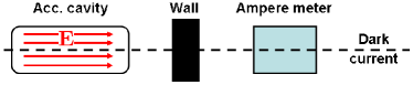
Figure 1: Schematic illustration of an accelerator cavity dark current (AC/DC) experiment for searching minicharged particles.

The basic setup for the experiment [10] is depicted in Fig. 1. In a strong electric field a vacuum pair of charged particles gains energy if the particles are separated by a distance along the lines of the electric field. If the electric field is strong enough (or the distance large enough) the energy gain can overcome the rest mass, i.e. the virtual particles turn into real particles. This is the famous Schwinger pair production mechanism [11]. After their production the electric field accelerates the particles and antiparticles according to their charge in opposite directions. This leads to an electric current (dashed line in Fig. 1). If the current is made up of minicharged particles the individual particles have very small charges and interact only very weakly with ordinary matter. Therefore, they can pass even through thick walls nearly unhindered. An electron current, however, would be stopped. After passage through the wall we can then place an ampere meter to detect the minicharged particle current.

Typical accelerator cavities achieve field strengths of $\gtrsim 25\,{\rm MeV/m}$ and their size is typically of the order of 10s of cm. Precision ampere meters can certainly measure currents as small as $\mu{\rm A}$ and even smaller currents of the order of ${\rm pA}$ seem feasible. Using the Schwinger pair production rate we can then estimate the expected sensitivity for such an experiment to be

$$\epsilon_{\rm sensitivity}\sim 10^{-8}-10^{-6}\quad{\rm for}\,\,m_{\epsilon}\lesssim{\rm meV}.$$ (19)

Therefore such an experiment has the potential for significant improvement over the currently best laboratory bounds shown in Fig. 2.

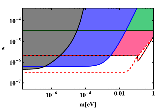
Figure 2: Laboratory bounds on minicharged particles. The black line (on the left, bottom solid) corresponds to the exclusion limit obtained in this note from the Cavendish type tests of Coulomb’s law [14, 15]. The blue bound (on the left, middle solid) arises from constraints on energy losses in high quality accelerator cavities [10]. The dark green curve (on the left, top solid) gives the limit arising from bounds on the invisible decay on orthopositronium [16, 17] (a similar bound can be obtained from a reactor experiment [18]). The red-black dashed line denotes the limit [19, 20] arising from light-shining-through-a-wall experiments [21, 22] and applies only to minicharged particles arising from kinetic mixing whereas the red dashed curve gives a limit [23, 20] from polarization experiments [21, 24]⁴ and applies for a pure minicharged particle scenario. The shaded areas are excluded in both scenarios.

Indeed, even without performing a dedicated experiment one can already obtain strong bounds from existing bounds on the energy loss in accelerator cavities [10]. The fact that high $Q$ values have been achieved at large field values strongly limits the energy loss into unknown sources such as minicharged particle production. The corresponding bound is shown as the blue region in Fig. 2.

5 Tests of Coulomb’s law as a probe for minicharged particles

Minicharged particles would also leave detectable footprints on the distance dependence of the electrostatic potential [15]. In presence of charged particles Coulomb’s law is modified due to the effects of the vacuum polarization $\Pi$. This is the so-called Uehling potential [26] (for a textbook derivation see, e.g., [27]),

$$V(\mathbf{x})=V_{\rm Coulomb}(x)+\delta V(x)=Q\int\frac{d^{3}q}{(2\pi)^{3}}\exp(i\mathbf{q}\cdot\mathbf{x})\frac{e^{2}}{|\mathbf{q}|^{2}(1-\Pi_{\epsilon}(q))}.$$ (20)

For large distances, $r\gg 1/m$, $\delta V$ drops off exponentially whereas for small distances, $r\ll 1/m$, it’s behavior is logarithmic as expected from the running gauge coupling,

$$\delta V(r)\!\! \approx \!\!\frac{Q\alpha}{r}\left[\frac{\alpha\epsilon^{2}}{4\sqrt{\pi}}\frac{\exp(-2mr)}{(mr)^{\frac{3}{2}}}\right]\quad\quad\quad\quad\quad\quad\quad\quad\quad\quad{\rm for}\quad\quad mr\gg 1,$$

$$\approx \!\!\frac{Q\alpha}{r}\left[-\frac{2\alpha\epsilon^{2}}{3\pi}\log(2mr)-a\right],\quad a\approx\frac{2\alpha\epsilon^{2}}{3\pi}\gamma\quad\quad\,\,{\rm for}\quad\quad mr\ll 1.$$

Due to their high mass electrons and heavier charged particles only lead to modifications of Coulomb’s law at extremely short distances. In contrast light minicharged particles could lead to modifications of Coulomb’s law at relatively large distances. We can therefore probe minicharged particles by testing Coulomb’s law.

One way to test Coulomb’s law is to use a so called Cavendish type experiment. Here, the electric potential between an outer charged conducting sphere and an uncharged inner sphere is measured. A specific feature of Coulomb’s law is that the electric potential inside a charged conductor is constant. Therefore, a non-vanishing voltage between the inner uncharged sphere and the outer sphere would indicate a deviation of Coulomb’s law.

By applying high voltages to the outer sphere and looking for minuscle voltages between the inner and the outer sphere experiments of this type have been performed with enormous precisions of up to about 2 parts in $10^{16}$ for sphere sizes of 10s of centimeters [14]. This leads to the black bound shown in Fig. 2.

6 Tunneling of the 3rd kind – Searching minicharged particles inside a superconducting box

Minicharged particles could also be searched for using a new type of tunneling process, “tunneling of the 3rd kind” [28]. This process is depicted in Fig. 3. Here, photons split into a virtual particle – antiparticle pair of charged particles which traverse an opaque wall and recombine after the wall into a photon. Due to their tiny interactions with ordinary matter the (virtual) minicharged particles can simply pass through the wall whereas photons would be stopped. After recombination the photons can then be detected. In this way minicharged particles lead to a light-shining-through-a-wall (LSW) signature. In contrast to the classical LSW process [29] (Fig. 3) where the photon is converted into a single real particle the intermediate particles are virtual. Accordingly, this process depends on the thickness of the wall.

To observe this process we would like to use a relatively thin wall that is nevertheless completely intransparent to the photons themselves. For optical frequencies this is rather difficult (among other things due to the high energy of the photons). Therefore, here we will consider an experiment using static magnetic fields shielded by a superconductor. The basic idea [30] of the proposed experiment is very similar to a classic LSW experiments [29]. However, instead of light it uses a static magnetic field and the wall is replaced by superconducting shielding (cf. Fig. 4). Outside the shielding we have a strong magnetic field. Upon entering the superconductor the ordinary electromagnetic field is exponentially damped with a length scale given by the London penetration depth $\lambda_{\rm Lon}$. Yet, due to tunneling of the 3rd kind a small fraction of the magnetic field penetrates the wall and can be detected by a magnetometer. Since the magnetometer measures directly the field (and not some probability or power output) the signal is proportional to the transition amplitude and therefore to the charge squared, $\epsilon^{2}$, instead of being proportional to $\epsilon^{4}$.

\begin{picture}(466.0,194.0)(42.0,-121.0) \put(0.0,0.0){} \put(0.0,0.0){} \put(0.0,0.0){} \put(0.0,0.0){} \put(0.0,0.0){} \put(0.0,0.0){} \put(0.0,0.0){} \end{picture}

\begin{picture}(466.0,194.0)(47.0,-121.0) \put(0.0,0.0){} \put(0.0,0.0){} \put(0.0,0.0){} \put(0.0,0.0){} \put(0.0,0.0){} \put(0.0,0.0){} \put(0.0,0.0){} \end{picture}

Figure 3: Left Panel: Diagram depicting a classical process for a penetration of the barrier via conversion into a real particle that interacts only very weakly with the barrier. Right Panel: Diagram depicting “tunneling of the 3rd kind”. The photon splits into a virtual pair of particle and antiparticle which traverse the wall and recombine into a photon.

High precision magnetometers can measure fields of the order of $10^{-13}$ T and even tiny fields of a few $10^{-18}$ T seem feasible. The expected sensitivity is of the order of $\epsilon\sim{\rm few}\times 10^{-7}$.

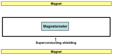
Figure 4: Sketched setup for the superconducting box experiment.

7 Searching minicharged particles with LSW experiments

In the previous section we have already encountered the possibility that minicharged particles can lead to a light-shining-through-a-wall signature. If there is also a light hidden U(1) gauge boson an additional process is possible and typically dominant: classical LSW via the hidden photon.

The essential process is depicted in Fig. 5. In presence of a non-vanishing magnetic background field the ordinary electromagnetic photon can be converted into a hidden photon via a minicharged particle loop [19]. The hidden photon can then traverse the wall and be reconverted on the opposite side of the wall via the inverse process. In terms of Fig. 3 the minicharged particle-loop is the (resolved) black dot and the hidden photon the dashed particle line.

Figure 5: The contribution of minicharged particles to the polarization tensor 5. The real part leads to birefringence, whereas the imaginary part reflects the absorption of photons caused by the production of particle-antiparticle pairs. The analogous diagram 5 shows how minicharged particles mediate transitions between photons and hidden-sector photons $\gamma^{\prime}$. Note that the latter diagram is enhanced with respect to the first one by a factor $\sim e_{\mathrm{h}}/(\epsilon e){=1/\chi}$. The double line represents the complete propagator of the minicharged particle in an external magnetic field $B$ as displayed in 5.

Currently a sizable number of LSW experiments [21] are under way [22]. They employ strong lasers as light sources and recycled magnets from accelerator experiments to provide for the magnetic field. Their power lies in the fact that they can put in $\gtrsim 10^{20}$ photons per second and are often able to detect $\lesssim 1$ photon per second.

The bounds arising from LSW experiments are shown as the red-black dashed line in Fig. 2. Let us note again, that this bound on minicharged particles relies on the presence of an extra hidden U(1) gauge boson. But, as we have seen in the first few sections, this is quite natural.

8 Searching minicharged particles with laser polarization experiments

Finally, let us turn to laser polarization experiments [21, 24]. In these experiments polarized laser light in shone through a strong magnetic field and changes in the polarization are searched for. These measurements can be used as sensitive probes of minicharged particles [23, 19, 20].

We can have two different types of changes in the polarization: a rotation of the linear polarization and a change into an elliptical polarization. In particular the rotation is (nearly) free of Standard Model backgrounds and therefore very suitable to probe for new physics [31]. As shown in Fig. 6 a selective absorption of one polarization direction via minicharged particle production results in a rotation of the linear polarization. A phase shift due to the vacuum polarziation leads to an ellipticity of the polarization.

Figure 6: Rotation (left) and ellipticity (right) caused by the existence of a light particle with a small electric charge (figure adapted from [32]). More precisely, the Feynman diagram in the left diagram corresponds to the imaginary part of Fig. 5 and the one in the right diagram corresponds to the real part of Fig. 5.

If there are only minicharged particles Fig. 6 describes the whole story. For this case we obtain the red-dashed bound in Fig. 2.

In presence of an additional hidden photon the situation is more complicated. Indeed one has to solve the full equations of motion arising from the diagrams shown in Fig. 5 [19]. As it turns out in this case the bounds are typically weaker than those obtained with other methods described above. This can serve as an example that the extra hidden photon can also “hide” some of the experimental signatures of minicharged particles. More positively, this also explicitly shows that we can experimentally distinguish between the two situations.

9 Conclusions

Minicharged particles are a natural candidate for physics beyond the Standard Model. Their embedding into extensions of the Standard Model as well as charge quantization tests suggest that they are accompanied by an extra U(1) gauge boson, the hidden photon.

Light minicharged particles can be searched for in a large variety of laboratory experiments using high precision measurements in strong electric and magnetic fields. Using different experiments it is possible to distinguish between a situation which only has minicharged particles and one where the minicharged particle is accompanied by a hidden photon.

It should be mentioned that for minicharged particles astrophysical bounds [12] are often considerably stronger than the current laboratory bounds. However, astrophysical bounds are also somewhat more model dependent [13]. Moreover, the recent rapid progress in the laboratory experiments raises the hope for considerable improvements in the near future.

Finally, the minicharged particles discussed in this note are only one example of a more general class of weakly interacting sub-eV particles (WISPs) that can be searched for in small scale laboratory experiments at low energies. Most of the above described experiments are also sensitive to other species of WISPs. For example, the extra hidden U(1) photon could also be massive. This leads to interesting effects such as photon – hidden photon oscillations even in absence of extra hidden matter that would become minicharged. For massive hidden photons experiments of the above described types provide the best bounds – even stronger than astrophysical bounds – for a large range of parameters.

With their small scale and rapid development low energy but high precision experiments inside strong elctromagnetic fields provide an interesting probe of physics beyond the Standard Model. They are not only complementary in the type of physics they probe but in addition they often recycle parts developed for accelerators such as high field magnets or high quality cavities.

Appendix A Alternative charge quantization arguments

In this appendix we will briefly consider alternative arguments for charge quantization and investigate how they are compatible with kinetic mixing.

A.1 A simple variant of the Dirac argument

In the main text we have used angular momentum quantization to argue in favor of charge quantization. Alternatively we can follow more closely Dirac’s original strategy [8] and look at gauge transformations.

Let us take a look at the gauge field configuration of a Dirac monopole. The gauge field for a Dirac monopole with its string pointing in the $\mathbf{n}$ direction is,

$$\mathbf{A}^{D}(\mathbf{r})=\frac{g}{4\pi}\frac{\hat{\mathbf{r}}\times\hat{\mathbf{n}}}{r(1-\hat{\mathbf{r}}\cdot\hat{\mathbf{n}})},$$ (22)

where the hat denotes unit vectors.

A Dirac monopole with its string pointing in the north pole direction $\mathbf{n}_{N}=(0,0,1)$ is physically equivalent to one with the string pointing in the south pole direction $\mathbf{n}_{S}=(0,0,-1)$. Therefore, they must be related by a gauge transformation,

$$\mathbf{A}^{D}_{N}-\mathbf{A}^{D}_{S}=\nabla\Lambda.$$ (23)

Under this gauge transformation the wave function of a particle with charge $q$ changes according to,

$$\psi\xrightarrow{\Lambda}\exp({\mathbf{i}}qe\Lambda)\psi.$$ (24)

Since the wave function must be a proper continuous function $\exp({\mathbf{i}}qe\Lambda)$ must be single valued.

Now let us calculate $\Lambda$ for our gauge transformation given by Eq. (23). Moving the particle from $\mathbf{x}_{0}$ to $\mathbf{x}$ the gauge phase changes by,

$$\Lambda(x)-\Lambda(\mathbf{x}_{0})=\int^{\mathbf{x}}_{\mathbf{x}_{0}}d\mathbf{s}\nabla\Lambda=\int^{\mathbf{x}}_{\mathbf{x}_{0}}d\mathbf{s}(\mathbf{A}^{D}_{N}-\mathbf{A}^{D}_{S}).$$ (25)

Now we can also imagine moving the particle around a closed loop. The single valuedness of the gauge transformation $\exp({\mathbf{i}}qe\Lambda)$ then requires

$$2\pi n=qe\oint d\mathbf{s}(\mathbf{A}^{D}_{N}-\mathbf{A}^{D}_{S}),\quad\quad n\in\mathbb{Z}$$ (26)

for any closed curve.

For our gauge transformation changing the direction of the string from the north to the south pole the right hand side of Eq. (26) can be easily evaluated for a closed curve around the equator and we obtain the charge quantization condition,

$$2\pi n=qeg.$$ (27)

In the case of minicharges with kinetic mixing we can now ask ourselves how this quantization condition is fulfilled. As with the angular momentum argument the trick is to take into account the effect of the hidden magnetic monopole field. For the ordinary electron which has no hidden electric charge the argument works as above. However, for the minicharged particle arising from kinetic mixing Eq. (26) picks up an additional contribution from the hidden monopole field,

$$2\pi n\!\! = \!\!\epsilon e\oint d\mathbf{s}(\mathbf{A}^{D}_{N}-\mathbf{A}^{D}_{S})+e_{h}\oint d\mathbf{s}(\mathbf{A}^{D,h}_{N}-\mathbf{A}^{D,h}_{S}),\quad\quad n\in\mathbb{Z}$$

$$= \!\!\epsilon eg+e_{h}g_{h}=-\chi e_{h}g+e_{h}g_{h}.$$

This is exactly equivalent to Eq. (17) and is automatically fulfilled if $g_{h}=\chi g$.

A.2 Charge quantization from the exclusion of black hole remnants

A completely different argument for charge quantization can be constructed by requiring that the theory is free of black hole remnants.

Let us assume for simplicity that we have only two types of particles with charge $q_{1}$ and $q_{2}$ with $q_{2}/q_{1}{\not\in}\mathbb{Q}$. Without restriction we can assume $q_{1}>q_{2}=1$. For simplicity we assume that they have the same mass $m$. Because the charge ratio is irrational we can make arbitrarily small total charges by combining a number $(n_{1},n_{2})$ or particles (and antiparticles)

$$1\gg Q_{tot}=n_{1}q_{1}+n_{2}q_{2}>0.$$ (29)

For each $\delta>0$ we can now find a combination such that $|n_{1}|+|n_{2}|=N_{min}(\delta)$ is minimal and $\delta\geq Q_{tot}\neq 0$. Neglecting the (small) interaction energy the energy of such a configuration is $N_{min}(\delta)m$.

However, on the other hand $N_{min}(\delta)$ depends on $\delta$ and goes to infinity as $\delta\to 0$. Therefore we can construct a series $\delta_{i}>0$ such that

$$\lim_{i\to\infty}\delta_{i}=0,\quad\quad N_{min}(\delta_{i+1})>N_{min}(\delta_{i})\quad\quad{\rm and}\quad\quad\lim_{i\to\infty}N_{min}(\delta_{i})\to\infty.$$ (30)

The last statement means that with increasing $i$ the energy of such configurations increases without bound.

Now, let us take such a configuration of charge $Q_{tot,i}\leq\delta_{i}$ and throw it into an uncharged black hole. Now this black hole can decay by emitting Hawking radiation of uncharged particles, e.g. photons, until it has reached an extremal Reissner-Nordstrom state with

$$\delta^{2}_{i}\geq Q^{2}_{tot,i}=M^{2}_{i}/M^{2}_{p},$$ (31)

and cannot decay any further without loosing charge. However, for sufficiently large $i$ (cf. Eq. (30)), $N_{min}(\delta_{i})m>M_{i}$ and the black hole also cannot shed charge by emitting charged particles because of energy conservation. In other words the created black hole is stable. Indeed we have an infinite number of such remnant states in the theory. This is in violation of our assumption that the theory is remnant free.

Again we can ask ourselves if minicharges arising from kinetic mixing can circumvent this charge quantization argument. Indeed they can. The reason is again that the electrically minicharged particles also have a hidden electric charge. A combination of particles with a smaller and smaller visible electric charge then must have higher and higher hidden charges. This modifies the condition for the charged black hole,

$$M^{2}/M^{2}_{P}\geq Q^{2}+Q^{2}_{h}.$$ (32)

Due to the high hidden charge the black hole now typically has enough energy/mass to decay directly into charged particles and thereby shed its charge, allowing for a complete decay.

References

- [1] B. Holdom, Phys. Lett. B 166 (1986) 196.
- [2] F. Brummer, J. Jaeckel and V. V. Khoze, JHEP 0906 (2009) 037 [arXiv:0905.0633 [hep-ph]].
- [3] B. Batell and T. Gherghetta, Phys. Rev. D 73 (2006) 045016 [hep-ph/0512356].
- [4] K. R. Dienes, C. F. Kolda and J. March-Russell, Nucl. Phys. B 492 (1997) 104 [hep-ph/9610479]; A. Lukas and K. S. Stelle, JHEP 0001 (2000) 010 [hep-th/9911156]; D. Lust and S. Stieberger, hep-th/0302221; S. A. Abel and B. W. Schofield, Nucl. Phys. B 685, 150 (2004) [hep-th/0311051]; S. Abel and J. Santiago, J. Phys. G 30, R83 (2004) [hep-ph/0404237]; R. Blumenhagen, G. Honecker and T. Weigand, JHEP 0506 (2005) 020 [hep-th/0504232]; R. Blumenhagen, S. Moster and T. Weigand, Nucl. Phys. B 751 (2006) 186 [hep-th/0603015]; S. A. Abel, J. Jaeckel, V. V. Khoze and A. Ringwald, Phys. Lett. B 666 (2008) 66 [hep-ph/0608248]; S. A. Abel, M. D. Goodsell, J. Jaeckel, V. V. Khoze and A. Ringwald, JHEP 0807 (2008) 124 [arXiv:0803.1449 [hep-ph]]; G. Dvali and M. Redi, arXiv:0905.1709 [hep-ph].
- [5] E. Witten, Phys. Lett. B 86 (1979) 283.
- [6] F. Brummer and J. Jaeckel, arXiv:0902.3615 [hep-ph].
- [7] H. A. Wilson, Phys. Rev. 75 (1949) 309; M. N. Saha, Indian J. Phys. 10 (1936) 145; Phys. Rev. 75 (1949) 1968; A. S. Goldhaber, Phys. Rev. 140 (1965) B1407.
- [8] P. A. M. Dirac, Proc. Roy. Soc. Lond. A 133 (1931) 60; Phys. Rev. 74 (1948) 817.
- [9] G. ’t Hooft, Nucl. Phys. B 79 (1974) 276; A. M. Polyakov, JETP Lett. 20 (1974) 194 [Pisma Zh. Eksp. Teor. Fiz. 20 (1974) 430].
- [10] H. Gies, J. Jaeckel and A. Ringwald, Europhys. Lett. 76 (2006) 794 [hep-ph/0608238].
- [11] J. Schwinger, Phys. Rev. 82 (1951) 664.
- [12] S. Davidson, S. Hannestad and G. Raffelt, JHEP 0005 (2000) 003 [hep-ph/0001179].
- [13] E. Masso and J. Redondo, JCAP 0509, (2005) 15, hep-ph/0504202; Phys. Rev. Lett. 97, (2006) 151802, hep-ph/0606163; J. Jaeckel, E. Masso, J. Redondo, A. Ringwald, and F. Takahashi, hep-ph/0605313; Phys. Rev. D75, (2007) 013004, hep-ph/0610203; P. Brax, C. van de Bruck, and A.-C. Davis, Phys. Rev. Lett. 99, (2007) 121103, hep-ph/0703243.
- [14] E. R. Williams, J. E. Faller and H. A. Hill, Phys. Rev. Lett. 26 (1971) 721; D. F. Bartlett and S. Loegl, Phys. Rev. Lett. 61 (1988) 2285.
- [15] J. Jaeckel, arXiv:0904.1547 [hep-ph].
- [16] A. Badertscher et al., Phys. Rev. D 75 (2007) 032004 [hep-ex/0609059].
- [17] A. Ringwald, private communication.
- [18] S. N. Gninenko, N. V. Krasnikov and A. Rubbia, Phys. Rev. D 75 (2007) 075014 [hep-ph/0612203].
- [19] M. Ahlers, H. Gies, J. Jaeckel, J. Redondo and A. Ringwald, Phys. Rev. D 76 (2007) 115005 [arXiv:0706.2836 [hep-ph]].
- [20] M. Ahlers, H. Gies, J. Jaeckel, J. Redondo and A. Ringwald, Phys. Rev. D 77 (2008) 095001 [0711.4991 [hep-ph]].
- [21] R. Cameron et al. [BFRT Collaboration], Phys. Rev. D 47 (1993) 3707.
- [22] K. Ehret et al. [ALPS Collaboration], hep-ex/0702023; C. Robilliard et al. [BMV Collaboration], Phys. Rev. Lett. 99 (2007) 190403; A. S. Chou et al. [GammeV (T-969) Collaboration], Phys. Rev. Lett. 100 (2008) 080402; P. Pugnat et al. [OSQAR Collaboration], arXiv:0712.3362 [hep-ex]. M. Fouche et al. [BMV Collaboration], Phys. Rev. D 78 (2008) 032013; A. Afanasev et al. [LIPSS Collaboration], Phys. Rev. Lett. 101 (2008) 120401; A. Afanasev et al. [LIPSS Collaboration], arXiv:0810.4189 [hep-ex]; K. Ehret et al. [ALPS Collaboration], arXiv:0905.4159 [physics.ins-det].
- [23] H. Gies, J. Jaeckel and A. Ringwald, Phys. Rev. Lett. 97 (2006) 140402 [hep-ph/0607118]; M. Ahlers, H. Gies, J. Jaeckel and A. Ringwald, Phys. Rev. D 75 (2007) 035011 [hep-ph/0612098].
- [24] E. Zavattini et al. [PVLAS Collaboration], Phys. Rev. Lett. 96 (2006) 110406 [arXiv:hep-ex/0507107]; S. J. Chen, H. H. Mei and W. T. Ni, Mod. Phys. Lett. A 22 (2007) 2815 [arXiv:hep-ex/0611050]; E. Zavattini et al. [PVLAS Collaboration], Phys. Rev. D 77 (2008) 032006 [arXiv:0706.3419 [hep-ex]].
- [25] D. Boer and J. W. Van Holten, arXiv:hep-ph/0204207. G. Zavattini and E. Calloni, Eur. Phys. J. C 62 (2009) 459 [arXiv:0812.0345 [physics.ins-det]]; B. Doebrich and H. Gies, arXiv:0904.0216 [hep-ph].
- [26] E. A. Uehling, Phys. Rev. 48 (1935) 55.
- [27] M. E. Peskin and D. V. Schroeder, “An Introduction To Quantum Field Theory,” Reading, USA: Addison-Wesley (1995) 842 p
- [28] H. Gies and J. Jaeckel, arXiv:0904.0609 [hep-ph].
- [29] L. B. Okun, Sov. Phys. JETP 56 (1982) 502 [Zh. Eksp. Teor. Fiz. 83 (1982) 892]. A. A. Anselm, Yad. Fiz. 42, 1480 (1985); M. Gasperini, Phys. Rev. Lett. 59, 396 (1987); K. Van Bibber, N. R. Dagdeviren, S. E. Koonin, A. Kerman and H. N. Nelson, Phys. Rev. Lett. 59, 759 (1987).
- [30] J. Jaeckel and J. Redondo, Europhys. Lett. 84 (2008) 31002 [arXiv:0806.1115 [hep-ph]].
- [31] M. Ahlers, J. Jaeckel and A. Ringwald, Phys. Rev. D 79 (2009) 075017 [arXiv:0812.3150 [hep-ph]].
- [32] F. Brandi et al., Nucl. Instrum. Meth. A 461 (2001) 329 [hep-ex/0006015].