Persistence of unvisited sites in presence of a quantum random walker

Abstract

A study of persistence dynamics is made for the first time in a quantum system by considering the dynamics of a quantum random walk. For a discrete walk on a line starting at $x=0$ at time $t=0$, the persistence probability $P(x,t)$ that a site at $x$ has not been visited till time $t$ has been calculated. $P(x,t)$ behaves as $(t/|x|-1)^{-\alpha}$ with $\alpha\sim 0.3$ while the global fraction ${\cal{P}}(t)=\sum_{x}P(x,t)/2t$ of sites remaining unvisited at time $t$ attains a constant value. $F(x,t)$, the probability that the site at $x$ is visited for the first time at $t$ behaves as $(t/|x|-1)^{-\beta}/|x|$ where $\beta=1+\alpha$ for $t/|x|>>1$, and ${\cal{F}}(t)=\sum_{x}F(x,t)/2t\sim 1/t$. A few other properties related to the persistence and first passage times are studied and some fundamental differences between the classical and the quantum cases are observed.

Various studies on persistence in dynamical systems have been made in recent years satya where the dynamical process is purely classical in nature. The persistence probability that the order parameter in a magnetic system has not changed sign till the present time derrida and the persistence of unvisited sites in a diffusion problem bray are common examples which have received extensive interest. The importance of persistence phenomena lies in the fact that the persistence probability in many systems shows an algebraic decay with a novel exponent.

The dynamics of a quantum system is expected to be different from the corresponding classical case. However, to the best of our knowledge no attempt to study persistence in quantum systems have been made so far. Here we report a study of persistence and related dynamical features in a quantum system which has a classial analogue such that it is possible to determine the differences, if any, between them.

The dynamical process we consider is a discrete quantum random walk (QRW). Classical random walk (CRW) on a line is a much studied topic chandra ; book ; redner where at every step one tosses a fair coin and takes a step, either to the left or right. In a quantum generalisation of a classical walk, one may consider superposition of particle movement in both directions, however such a process is physically impossible due to non-unitarity. A QRW in one dimension thus involves a quantum particle on a line with an additional degree of freedom which may be called chirality nayak ; kempe . The chirality takes values left and right analogous to Ising spin states $\pm 1$, and directs the motion of the particle. At any given time, the particle is in a superposition of left and right chirality. Thus the wave function has two components and at each time step, the chirality undergoes a rotation (a unitary transformation in general) and the particle moves according to its final chirality state.

The reason to study the qunatum random walk is that it is already known to have some distinctive behaviour when compared to the classical walk. While in the CRW, after $t$ time steps, the variance $\sigma^{2}\propto t$, the quantum walker propoagates much faster with $\sigma\propto t$. This feature of faster flow of a quantum walker has made its application in quantum computation highly relevant. Moreover, the QRW spreads roughly uniformly over the interval $[-t/\sqrt{2},t/\sqrt{2}]$ whereas in the classical case the distribution is peaked at the origin and drops off exponentially fast.

In the case of the classical random walker, the well studied quantities are (a) the first passage time $F_{cl}(x,t)$ which is the probability that the walker has reached the site $x$ for the first time at time $t$ redner and (b) persistence or the survival probability $P_{cl}(x,t)$ defined as the probability that the site at $x$ has not been visited till time $t$ chandra ; book . A related quantity is the average persistence probability given by $\sum_{x}P_{cl}(x,t)/L$ (where $x$ can take values from $-L/2$ to $L/2$). This quantity is global and can be interpreted as the fraction of sites remaining unvisited till time $t$.

In this paper, we have studied both the first passage probabilities and the persistence probabilities of sites in presence of a quantum random walker. Not only do we find out $F(x,t)$ and $P(x,t)$ as functions of $t$ and $x$, we also observe several other interesting features of the distributions which indicates that there are two independent dynamical exponents for the quantum random walker.

In this context, it may be mentioned that in the QRW, the walks can be realized in several possible ways, e.g., a walk can be infinite timed in which the walk is allowed upto time $t$ at which all measurements are made. Another method may be to have a semi infinite walk where the question is asked at every time step whether the walker is in a specific location, and if it is so, the system is allowed to collapse to that state. In our case, we simply evaluate the occupation probabilities at each step for each discrete location and calculate the persistence and first passage probabilities which are related to it. There is no actual measurements being made which will lead to a collapse to any particular state. Rather, our calculations will correspond to what would be the result of repeated experiments.

The states for a quantum random walker are written as $|x\rangle|d\rangle$ where $x$ is the location in real space and the $d$ the chirality having either “left” and “right” values. The chiral states are denoted as $|L\rangle$ and $|R\rangle$. A conventional choice of the unitary operator causing the rotation of the chirality state is the Hadamard coin represented by

$$H=\frac{1}{\sqrt{2}}\begin{pmatrix}1&1\\ 1&-1\end{pmatrix}.$$ (1)

The rotation is followed by a translation represented by the operator $T$:

$$\begin{array}[]{l}T|x\rangle|L\rangle\rightarrow|x-1\rangle|L\rangle\\ T|x\rangle|R\rangle\rightarrow|x+1\rangle|R\rangle\\ \end{array}.$$ (2)

The two component wave function $\psi(x,t)$ describing the position of the particle is written as

$$\psi(x,t)=\begin{pmatrix}\psi_{L}(x,t)\\ \psi_{R}(x,t)\end{pmatrix},$$ (3)

and the occupation probability is given by

$$f(x,t)=|\psi_{L}(x,t)|^{2}+|\psi_{R}(x,t)|^{2}.$$ (4)

Normalisation of the probability implies that at every step $\sum_{x}f(x,t)=1$.

We have used two methods to evaluate $f(x,t)$:
 1. A quantum random walk is generated using the above operators and $\psi_{L}(x,t)$ and $\psi_{R}(x,t)$ are evaluated numerically for all $x$ and $t$. We start with the walker at the origin with $\psi_{L}(0,0)=a_{0},\psi_{R}(0,0)=b_{0};~{}~{}a_{0}^{2}+b_{0}^{2}=1$ and all other $\psi_{L}$ and $\psi_{R}$ taken equal to zero.
2. In the second method we use the expressions nayak

$$\psi_{L}(x,t)=\frac{1+(-1)^{x+t}}{2}\int\frac{dk}{2\pi}(1+\frac{\cos k}{\sqrt{1+\cos^{2}k}})e^{-i(\omega_{k}t+kx)}$$ (5)

$$\psi_{R}(x,t)=\frac{1+(-1)^{x+t}}{2}\int\frac{dk}{2\pi}\frac{e^{ik}}{\sqrt{1+\cos^{2}k}}e^{-i(\omega_{k}t+kx)}$$ (6)

(which are obtained for a initial state with left chirality, i.e., $a_{0}=1,b_{0}=0$) and evaluate $f(x,t)$ directly.

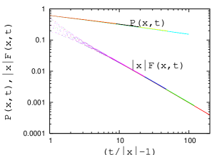
Figure 1: The data collapse for the persistence probability and scaled first passage probability for a quantum random walk shown for different values of $x$.

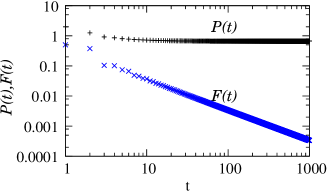
Figure 2: Plot of average persistence ${\cal{P}}(t)$ and first passage time ${\cal{F}}(t)$ indicate ${\cal{P}}(t)$ is approaching a constant for large time whereas ${\cal{F}}(t)$ behaves as $t^{-1}$.

The persistence probability that a site $x$ has not been visited till time $t$, is given by in terms of the occupation probabilities:

$$P(x,t)=\prod_{t^{\prime}=1}^{t}(1-f(x,t^{{}^{\prime}})),$$ (7)

while the first passage time

$$F(x,t)=\prod_{t^{\prime}=1}^{t-1}(1-f(x,t^{{}^{\prime}}))f(x,t)$$ (8)

$$=P(x,t-1)f(x,t).$$

Some time dependent features like hitting time, recurrence time etc. hitting ; Stefanak of the QRW have been studied earlier which involve the first passage time. However, in these studies, the spatial dependence has not been considered. For example, quantities like first passage time specifically at the origin has been estimated.

In the first method of calculation, in general, real values of the coefficients $a_{0}$ and $b_{0}$ give an asymmetric result for $f(x,t)$ in the sense the occupations probabilities $f(x,t)\neq f(-x,t)$ as there is destructive interference. However, taking specific complex values of $a_{0}$ and $b_{0}$ or by taking a different coin results in a symmetric walk kempe .

We first discuss the results for the symmetric case obtained by taking $a_{0}=1/\sqrt{2},b_{0}=i/\sqrt{2}$. We find that $P(x,t)$ and $F(x,t)$ as functions of $t$ and $x$ behave as

$$P(x,t)\propto(t/|x|-1)^{-\alpha}$$ (9)

for $t/|x|>1$, and

$$F(x,t)\propto(t/|x|-1)^{-\beta}/|x|$$ (10)

for $t/|x|>>1$ with $\alpha\simeq 0.31$ and $\beta\simeq 1.31$. The data collapse for $P(x,t)$ and $F(x,t)$ are shown in Fig. 1.

Using the above form of $P(x,t)$, the average probability ${\cal{P}}(t)$ that a site is unvisited till time $t$ is given by $\sum_{x=-t}^{t}P(x,t)/2t$ (since $x$ can assume discrete values from $-t$ to $+t$) which in the symmetric case is approximately equal to

$$\frac{1}{t}\int_{0}^{t}P(x,t)dx=\frac{A}{t}\int_{0}^{t}(\frac{t}{x}-1)^{-\alpha}dx.$$ (11)

The integral on the rhs of eq (11) can be done exactly giving a constant value equal to 0.738 (using $A=0.626$ which we get from the fitting of $P(x,t)$ shown in Fig.1), indicating that ${\cal{P}}(t)$ is time independent. We indeed find by numerically evaluating $\sum_{x=0}^{t}P(x,t)/t$ that it approaches a constant value as $t$ becomes large. The constant is $\approx 0.66$, quite close to the value obtained above. On the other hand, $\sum_{x=-t}^{t}F(x,t)/2t$ varies as $t^{-1}$, a result which can be obtained using a similar approximation and also obtained numercially. The numerical results are shown in Fig. 2.

The function $F(x,t)$ in fact has some additional features. Plotting $F(x,t)$ against $x$ or $t$, we notice that it has an oscillatory behaviour. These oscillations which die down for large values of $t/x$ as is apparant from Fig. 1 can be traced to the oscillatory behaviour of $f(x,t)$ for a QRW observed earlier nayak ; kempe . From Figs 3 and 4, we observe that $F(x,t)$ actually attains a maximum value $F_{max}(x,t)$ at values of $|x|=x_{max}$ (or $t=t_{max}$) for fixed values of $t$ (or $x$). We notice that $F_{max}(x_{max},t)\propto x_{max}^{-\delta}$ where $\delta\simeq 0.59$. Keeping $x$ fixed, $F_{max}(x,t_{max})$ versus $t_{max}$ shows the same kind of dependence, i.e., $F_{max}(x,t_{max})\propto t_{max}^{-\delta}$. That the scalings with $t_{max}$ and $x_{max}$ turn out to be identical is not surprising as $x$ scales as $t$ in a QRW. It is not possible to obtain this scaling form directly from eq. (10) since $F(x,t)$ attains a maximum value when $t/|x|$ is close to unity where the fitted scaling form is not exactly valid. In fact, eq. (10) does not give any maximum value at all.

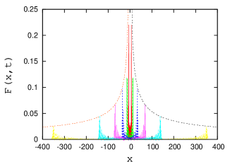
Figure 3: Typical variation of $F(x,t)$ against $x$ for different values of $t$. The peaks are approximately fitted to $0.81x_{max}^{-0.59}$.

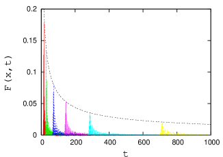
Figure 4: Typical variation of $F(x,t)$ against $t$ for different values of $x$. The peaks are approximately fitted to $t_{max}^{-0.59}$.

Another dynamic quantity called hitting time has been estimated earlier for the QRW, in which an absorber is assumed to be located at a specific vertex of a hypercube within which the walk is conceived hitting . The average hitting time is by definition the average time to reach that particular vertex for the first time. One can evaluate the average hitting time $\tau_{h}(x)$ using $\tau_{h}(x)=\sum_{0}^{T}tF(x,t)$ where $t$ is allowed to vary from $0$ to $T$:

$$\tau_{h}\approx\int_{0}^{T}tF(x,t)dt$$

$$\sim{T}^{2-\beta}x^{\beta-1}/(2-\beta)+O({T}^{-{\beta+1}}).$$

The numerical data (not shown) gives a fairly good agreement with this scaling. The above equation shows that $\tau_{h}$ blows up for $T\to\infty$ in agreement with some earlier results using other coins hitting .

When $a_{0}$ and $b_{0}$ are allowed to take up real values, in general the probability $f(x,t)$ is asymmetric. Now we study the behaviour of $P(x,t)$ and $F(x,t)$ for $x>0$ and $x<0$ independently. In particular, we find that when there is a left bias, i.e., the probability that $f(x<0,t)>f(x>0,t)$, $P(x<0,t)$ is less than $P(x>0,t)$, which is to be expected. Moreover, the scaling behaviour for $x<0$ shows an additional dependence on $x$, $P(x<0,t)$ is now given by

$$P(x,t)\propto(t/|x|-1)^{-\alpha}|x|^{p}$$

where $p$ is approximately 0.03 for $a_{0}=1$, $b_{0}=0$. If $a$ and $b$ are chosen differently, the value of $p$ shows up a variation with the chosen values, however it is still $O(0.01)$. Such a small value of $p$ suggests that this could be due to numerical errors. Fig. 5 shows the left-right persistence behaviour.

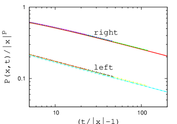
Figure 5: Data collapse of $P(x,t)$ for a quantum random walk with a left bias. For the right side data, $p=0$ and for the left side, $p=0.03.$

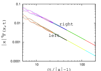
Figure 6: Data collapse of $F(x,t)$ for a quantum random walk with a left bias. For the right side data, $q=1$ and for the left side, $q=1-0.07$

The first passage probability for $x<0$ shows a similar correction to scaling

$$F(x,t)\propto(t/|x|-1)^{-\beta}|x|^{-q}$$

where $q=1-O(0.01)$ Fig. 6 shows typical variations of $F(x,t)$ for $a_{0}=1$, $b_{0}=0$ with $q=0.93$ .

The significance of the various results obtained in the present work becomes quite clear when these are compared to those of the classical random walker. For a CRW, the first passage time $F_{cl}(x,t)$ is known exactly chandra ; book

$$F_{cl}(x,t)={\rm{const}}\frac{|x|}{t^{3/2}}\exp(-x^{2}/Dt),$$

where $D$ is a diffusion constant. Hence $F(x,t)$ behaves as $t^{-3/2}$ for large $t$. The persistence or survival probability is given by ${\rm{erf}}(\frac{|x|}{\sqrt{Dt}})$ which behaves as $|x|t^{-1/2}$ as $t\to\infty$. In fact the two quantities, persistence probability and first passage time are related in the continuum limit:

$$F(x,t)=-\frac{\partial P(x,t)}{\partial t},$$ (12)

and hence the scaling behaviour (with time) of $F$ can be found out from that of $P$ or vice versa; e.g., $\beta_{cl}=\alpha_{cl}+1$, where $P_{cl}\propto t^{-\alpha_{cl}}$ and $F_{cl}\propto t^{-\beta_{cl}}$.

In general one can write $x\propto t^{\gamma}$ for these kind of dynamical phenomena where the inverse of $\gamma$ is a dynamical exponent. It can be expected that the scaling behaviour of all other quantities will be dictated by the exponent $\gamma$. Here we would like to emphasise that while this is true for the classical case, for the QRW, that is not the case. Let us consider each physical measure for the CRW and QRW to establish this claim.

In the CRW, $\gamma=\gamma_{cl}=1/2$ and the scaling of the first passage time with time occurs with an exponent $\beta_{cl}=3\gamma_{cl}$ and the persistence probability with an exponent $\alpha_{cl}=\gamma_{cl}$. For the quantum walker, $\gamma=\gamma_{q}=1$, however, the persistence behaviour and the first passage times vary in time with exponents $\alpha$ and $\beta$ which are not simple multiples of $\gamma_{q}$ although $F(x,t)$ and $P(x,t)$ indeed obey the relation given in eq. (12) such that $\beta=1+\alpha$. The form of the persistence probability and first passage time are in fact entirely different from those of the classical case as indicated by the collapsed data.

In the classical case, the global fraction ${\cal{F}}_{cl}$ behaves as $t^{-1}$. From this, one can infer that the global fraction ${\cal{P}}_{cl}$ is approximately a constant. In the quantum case, surprisingly, we have identical scaling behaviour for ${\cal{P}}(t)$ (which saturates to a constant value) and ${\cal{F}}(t)$ (which varies as $t^{-1}$). In terms of $\gamma$ however, ${\cal{F}}_{cl}\propto t^{-2\gamma_{cl}}$ while ${\cal{F}}\propto t^{-\gamma_{q}}$. In the QRW a striking feature is that these global properties do not involve the exponents $\alpha$ and $\beta$ at all and only $\gamma_{q}$ dictates their behaviour.

Concerning the maximum values of the classical probability $F_{cl}$, we find that it behaves as $1/t_{max}$ (for $x$ constant) or $1/x_{max}^{2}$ (for $t$ constant) showing that the obtained exponents are simple multiples of $\gamma_{cl}=1/2$. On the other hand, the behaviour of $F_{max}$ in the quantum case appears to depend on the value of $\alpha$ and not $\gamma_{q}$ as it varies with ${t_{max}}$ or $x_{max}$ with an exponent $\delta$ which is very close to $2\alpha$ numerically.

The average hitting time for a CRW is found to vary as $T^{\gamma_{cl}}$. In the QRW, this variation is given by $T^{2-\beta}$. For the classical case, $2-\beta_{cl}=\gamma_{cl}$ but since no such relation exists for the quantum case, the hitting time scaling is therefore not dictated by $\gamma_{q}$ but by $\beta$ (or $\alpha$) only.

Thus the scaling forms of different quantities for the quantum and classical walks are not identical in general and the scaling behaviour in the quantum case is dictated either by $\gamma_{q}$ or by $\alpha$. From this we draw the important conclusion that there are two nontrivial and independent exponents for the QRW in contrast to the CRW. This result may have serious impact on quantum computational aspects.

Acknowledgement: Financial supports from DST grant no. SR-S2/CMP-56/2007 (PS) and UGC sanction no. UGC/209/JRF(RFSMS) (SG) are acknowledged.

References

- (1)
- (2) S.N. Majumdar, Curr. Sci. 77 370 (1999).
- (3) B. Derrida, A.J.Bray and C. Godreche, J.Phys. A 27 L357 (1994).
- (4) S. J. O’Donoghue and A. J. Bray, Phys. Rev. E 64, 041105 (2001); P. K. Das, S. Dasgupta and P. Sen, J. Phys. A: Math. Theor. 40 6013 (2007).
- (5) S. Chandrasekhar, Phys. Rev.,15 1 (1943).
- (6) G. H. Weiss, Aspects and applications of the random walk, North Holland, Amsterdam (1994).
- (7) S. Redner, A guide to first-passage processes,, Cambridge University Press, (2001).
- (8) A. Nayak and A. Vishwanath, DIAMCS Technical Report 2000-43 and Los Alamos preprint archive,quant-ph/001017; A. Ambanis, E. Bach, A. Nayak, A. Vishwanath and J. Watrous, Proc. 33th New York, NY (2001).
- (9) J. Kempe, Contemporary Physics 44 307-327 (2003).
- (10) H. Krovi and T.A. Brun, Phys. Rev. A 73 032341 (2006); J. Kempe, arXiv quant-ph/0205083.
- (11) M. Stefanak, I. Jex, T. Kiss, Phys. Rev. Lett 100 020501 (2008); C. M. Chandrashekar, arXiv:0810.5592, v2 01 (2008).