Hydrodynamics of Strongly Coupled Non-conformal Fluids from Gauge/Gravity Duality

Abstract

The subject of relativistic hydrodynamics is explored using the tools of gauge/gravity duality. A brief literature review of AdS/CFT and gauge/gravity duality is presented first. This is followed by a pedagogical introduction to the use of these methods in determining hydrodynamic dispersion relations, $w(q)$, of perturbations in a strongly coupled fluid.

Shear and sound mode perturbations are examined in a special class of gravity duals: those where the matter supporting the metric is scalar in nature. Analytical solutions (to order $q^{4}$ and $q^{3}$ respectively) for the shear and sound mode dispersion relations are presented for a subset of these backgrounds.

The work presented here is based on previous publications by the same author [1], [2], and [3], though some previously unpublished results are also included. In particular, the subleading term in the shear mode dispersion relation is analyzed using the AdS/CFT correspondence without any reference to the black hole membrane paradigm.

University of Minnesota Physics

August 2009

331 I would like to thank R. Anthony, E. Aver, A. Buchel, T. Cohen, A. Cherman, T. Kelley, M. Natsuume, D. T. Son, and A. Starinets for helpful comments, suggestions and discussions regarding the work presented here.

I thank the members of my examination committee: D. Cronin-Hennessey, L.L.R. Williams, and M. Peloso for their time and consideration

I would also like to thank T. Gherghetta, R. Fries and S. Barthel for their help in transitioning to life after graduate school.

Finally, I gratefully acknowledge the support and guidance of my adviser J. I. Kapusta who has provided invaluable insight and feedback on all aspects of my graduate school career.

This work was was supported by the US Department of Energy (DOE) under Grant. NO. DE-FG02-87ER40328, and by the Graduate School at the University of Minnesota under the Doctoral Dissertation Fellowship.

To my parents, who have provided me with unconditional support over the years.

Chapter Introduction

Each of the fundamental forces in nature is currently understood in the context of a particular theory. Gravity is understood in terms of Einstein’s theory of general relativity (the quantum theory of gravity is currently unknown, and highly sought after); while the electromagnetic and weak forces are both understood in the context of the standard model of electroweak interactions. The subject of this research is the theory of the strong nuclear force, Quantum Chromodynamics (QCD).

QCD is the theory of the interaction that binds protons and neutrons together to form atomic nuclei. Quarks (fermions), and gluons (gauge bosons of the underlying SU(3) gauge group) are the fundamental constituents of the theory. It is believed that if one heats normal matter to high enough temperatures, or compresses it to high enough densities, a new state of matter is formed wherein the boundaries between particular nucleons are no longer well defined. Instead of a sea of nucleons, one finds a “soup” of quarks and gluons. We will refer to this state of matter as quark-gluon plasma (QGP) It is believed to have dominated the universe in the first few microseconds after the Big Bang.

Experimentalists are attempting to re-create this environment using particle accelerators which smash nuclei into each other at very high energies. In the last few years, there is evidence that the Relativistic Heavy Ion Collider (RHIC) at Brookhaven National Laboratory has created such a state of matter [4, 5, 6, 7].

The plasma created at RHIC exhibits some surprising properties. In particular, observation of strong collective behavior (elliptic flow), and the large energy loss of high energy particles traversing the medium (jet quenching) indicate that the plasma interacts very strongly with itself, and is thus referred to as strongly coupled. This presents a problem for theoretical physicists, because the equations of QCD cannot be solved analytically in this regime; traditional approximation techniques involve a perturbative expansion in the coupling constant which measures the strength of the interaction. If the coupling constant is large (i.e. $\mathcal{O}(1)$), such a perturbative expansion is unreliable, as each successive term in the series becomes larger than the previous one, and the approximation scheme breaks down. This difficulty with QCD has plagued theorists for over 30 years since the inception of the theory.

However, in the late 1990’s, new techniques were developed which attempt to address these non-perturbative problems [8, 9, 10]. In particular, it has been conjectured that there is a duality between certain strongly coupled gauge theories and weakly coupled string theories. By this, it is meant that both theories may describe the same physics, but calculations may be easier in one theory than the other. As mentioned above, it has been argued that the duality is a weak/strong type, such that when one theory is strongly coupled, the other is weakly coupled and vice-versa. One can immediately see the possible application to QCD; if a dual theory to QCD is found, one can do computations in the dual theory (at weak coupling, where calculations are possible), instead of in QCD itself (at strong coupling where calculations are difficult).

Much work needs to be done before we can apply these ideas to real-world QCD. At the present time, the duality (referred to in the title as the gauge/gravity correspondence) is well developed for a theory which shares some properties with QCD, but lacks some of the essential features that we observe in the real world. Attempts are currently being made to both search for a dual theory of QCD, and to modify the idealized theory to make it more physically relevant.

The ultimate goal of this line of research is the calculation of observable properties of the quark-gluon plasma. This is still a difficult task, because the string dual to QCD is not currently known. In light of this fact, there are two avenues which one may pursue. First, one can attempt to compute observables in phenomenologically motivated extra-dimensional models of QCD. The drawback here is that at the present time, such models are lacking from a theoretical point of view. Secondly, one can attempt to look for universal features of strongly coupled theories, which might then also be applicable to QCD.

Here we employ the latter approach; we search for universal behavior in hydrodynamic transport coefficients which describe a fluid’s response to small perturbations. Hydrodynamics is an effective theory of fluids in thermal equilibrium. It is applicable when macroscopic length and time scales of interest are much longer than any microscopic scale. In this regime, the effective stress-energy tensor can be constructed as a derivative expansion in the fluid velocity. Naturally, such an effective construction introduces unknown coefficients. These are the transport coefficients mentioned above, and which will be discussed in much greater detail in the coming chapters.

These coefficients are necessary input for hydrodynamical simulations of the quark-gluon plasma. Currently, we understand that a heavy ion collision occurs in roughly three distinct phases. Before the collision, the two colliding nuclei are highly Lorentz contracted, but have not yet entered into thermal equilibrium; in this phase, the nuclei can be described within the framework of, for example, the Color Glass Condensate [11]. After the collision, some of the energy of the colliding nuclei is transformed into a bath of new particles, which rapidly thermalizes. Once the new system has reached thermal equilibrium, a hydrodynamic description is appropriate. The newly created region of quark-gluon plasma then expands and cools; once it has cooled enough, it drops out of thermal equilibrium and the matter hadronizes into particles which are then detected. Describing the initial (pre-equilibrium) and final (freeze out) stages of the heavy ion collision is a difficult and very active area of research, it is also beyond the scope of this thesis - for reviews, see [12, 13, 14]. Luckily, it appears that there is a stage of the heavy ion collision when the matter is thermally equilibrated, and thus admits a hydrodynamic description. It is in this phase of the collision that one needs to specify the relevant transport coefficients. It is thus desirable to calculate these coefficients, but as mentioned above, the strong coupling of the plasma renders traditional perturbative calculations unreliable. Thus, one is led to try using gauge/gravity duality methods to compute such quantities.

The thesis is organized as follows

• In Chapter Hydrodynamics of Strongly Coupled Non-conformal Fluids from Gauge/Gravity Duality, we give a brief review of the motivation, and some of the basic tools of gauge/gravity duality. While hydrodynamics and transport coefficients are the main focus of this work, in this section we also discuss some other applications of gauge/gravity duality to strongly coupled plasma. Particular attention is paid to thermodynamic applications, some of which are useful in later chapters.

• In Chapter Hydrodynamics of Strongly Coupled Non-conformal Fluids from Gauge/Gravity Duality, we explain the relevant background material regarding hydrodynamics. We also discuss some of the standard methods of computing transport coefficients from gauge/gravity duality, and explain in detail the method which will be used in deriving the central results of the thesis.

• In Chapters Hydrodynamics of Strongly Coupled Non-conformal Fluids from Gauge/Gravity Duality and Hydrodynamics of Strongly Coupled Non-conformal Fluids from Gauge/Gravity Duality, the techniques described above are applied to a particular class of dual theories. These sections contain the central results of this thesis. We derive equations which are applicable to a wide variety of gravitational dual theories, and could in principle be used within the context of phenomenological models of QCD. We also apply these equations to a few analytically solvable special cases, and examine the results to determine if any universal features of strongly coupled plasmas are manifest. The methodology employed in each of these chapters is the same, but each one concerns a different type of hydrodynamic perturbation. In Chapter Hydrodynamics of Strongly Coupled Non-conformal Fluids from Gauge/Gravity Duality we study shear perturbations while sound (or compressional) perturbations are studied in Chapter Hydrodynamics of Strongly Coupled Non-conformal Fluids from Gauge/Gravity Duality.

• Finally, in Chapter Hydrodynamics of Strongly Coupled Non-conformal Fluids from Gauge/Gravity Duality, we discuss the main conclusions of the analysis and also mention open questions and prospects for future investigation.

Chapter Gauge/Gravity Duality: An Overview

In this chapter, we first explain the basics of gauge/gravity duality, and the AdS/CFT (Anti-de Sitter/Conformal Field Theory) correspondence. The focus of this thesis is phenomenology, and particular applications of the correspondence, so many of the details regarding the foundations of the duality will not be presented here. Relevant references are provided for the interested reader. Some excellent reviews of the subject which parallel the present discussion can be found in [15, 16, 17, 18, 19].

Once the basics of the duality have been established, we present a review of the relevant literature regarding applications of the duality (mass spectra, form factors, jet quenching, etc.). The main application discussed in this thesis (hydrodynamic dispersion relations and transport coefficients) will be explored in more detail in the next chapter.

Finally, we discuss in some detail applications of the duality to thermodynamic aspects of the relevant gauge theory. Many of these results will be useful in subsequent chapters.

1 What is Gauge/Gravity Duality?

The original motivation for gauge/gravity duality came from considerations of type IIB string theory, which exists in ten dimensions. It is not necessary to understand the details of string theory for this derivation, but one should appreciate that it is a theory which contains strings, but also extended membrane like objects, branes. D-branes are such objects which can serve as endpoints for the strings (‘D’ stands for Dirichlet). The theory has two types of excitations, closed strings which have no endpoints, and open strings which are allowed to have endpoints on a D-brane. Strings are characterized by their length $l_{s}$, and the coupling constant which controls the strength of their interaction is denoted $g_{s}$. The string coupling can be related to the $D$ dimensional Newton’s gravitational constant $G_{D}$ by

$$G_{D}\propto g_{s}^{2}l_{s}^{D-2}.$$ (1)

To proceed, let us consider type IIB string theory in the background of a system of $N$ D3-branes stacked on top of one another. (A D3-brane is a D-brane which extends in three spatial dimensions). We will now consider the low energy dynamics of this system from two different viewpoints.

First, the low energy excitations of open strings on the system of $N$ D3-branes can be described by a $SU(N)$ gauge theory. Specifically, the relevant low energy effective theory is $\mathcal{N}=4$ supersymmetric Yang-Mills (hereafter SYM) theory.The gauge coupling $g_{YM}$ is related to the string coupling $g_{s}$ as [20],

$$g^{2}_{YM}=4\pi g_{s}.$$ (2)

If we consider the string length to be small, then we can neglect any interactions between the branes and the closed strings which exist outside of the branes (in the region called the bulk). We can also neglect any interactions among the closed strings themselves. This is because all interaction terms will contain positive powers of the gravitational coupling $G_{D}$. If we are interested in processes which have typical energy $E$ much smaller than the Planck mass $M_{p}$, these interaction terms will be suppressed by powers of $E/M_{p}$. Thus, from this point of view, the low energy limit of this entire system consists of two decoupled pieces: free low energy closed string theory (type IIB supergravity) in the bulk, and $\mathcal{N}=4$ SYM theory on the branes. This point of view is presented in graphical form in Fig. 1.

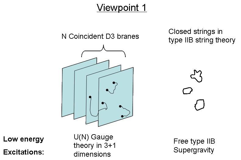
Figure 1: Type IIB string theory in the background of a set of N coincident D3 branes. Low energy excitations of this system decouple into the two pieces shown above; the low energy excitations of the brane system are those of a gauge theory.

Now, consider this system from an alternative point of view. If $N$ is very large, the stack of branes will have a considerable amount of energy, and thus will curve space-time in accordance with general relativity. In [21], it was shown that one can find black hole type solutions to these supergravity equations. The classical metric which solves the supergravity equations can be written

$$ds^{2}=\frac{1}{\sqrt{1+L^{4}/r^{4}}}\left(-dt^{2}+d\vec{x}^{2}\right)+\sqrt{1+\frac{L^{4}}{r^{4}}}\left(dr^{2}+r^{2}d\Omega_{5}^{2}\right),$$ (3)

where $L$ is the only scale, and is the so called curvature radius. The vector $\vec{x}$ runs over the three spatial coordinates, and $\Omega_{5}$ is the five dimensional angular element. In addition to this metric, there is a scalar field (dilaton), and a five-form, but these additional fields are unimportant for the argument here. From this point of view, the system now has two types of low energy excitations: closed string excitations which are far away from the brane which is located at $r=0$, or any sort of excitation near the location $r=0$. From the point of view of an observer at $r=\infty$, these excitations appear to be low energy due to the gravitational redshift from the metric. In the near horizon regime $r<<L$, the metric becomes

$$ds^{2}=\frac{r^{2}}{L^{2}}\left(-dt^{2}+d\vec{x}^{2}\right)+\frac{L^{2}}{r^{2}}dr^{2}+L^{2}d\Omega_{5}^{2},$$ (4)

which is the product of five dimensional anti-de Sitter space, with a 5-sphere ($AdS_{5}\times S_{5}$). (Anti-de Sitter space is a maximally symmetric metric which is a solution to Einstein’s equations with a negative cosmological constant).

Furthermore, both of the types of excitations listed above decouple if the energy is low enough, because the wavelength of the closed string excitations will be larger than the gravitational size of the branes ($\sim L$). This point of view is presented graphically in Fig. 2.

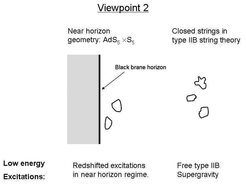
Figure 2: The same system as in Fig. 1, viewed in a different way. If the stack of branes is large, they curve space-time and can be described by a classical metric. The gravitational redshift causes excitations near the horizon to appear very low in energy.

Now let us compare the two viewpoints of this system. In each description there are two decoupled pieces. In the first system, the decoupled pieces are the $\mathcal{N}=4$ SYM gauge theory, and low energy closed string excitations. In the second description, the decoupled pieces are the excitations in the near horizon regime of the black hole, and low energy closed string excitations far away from the horizon. Maldacena’s conjecture is that these two systems should describe the same physics [8]. Each of the two descriptions has low energy closed string excitations as one element, thus we should equate the remaining two elements. The result is the conjecture that $\mathcal{N}=4$ SYM theory is dual to type IIB string theory on $\mathbf{AdS_{5}\times S_{5}}$.

To see why this is useful, consider describing the type IIB string theory by a classical supergravity metric (4) and associated supergravity fields. In other words, we neglect all stringy effects and treat the theory classically. When is such an approximation valid? Clearly, one must have the string length much less than the curvature radius:

$$l_{s}\ll L.$$ (5)

We can relate this to the parameters of the gauge theory by examining the total energy/volume of the stack of branes within these two different viewpoints.

On one hand, the total energy/volume of the brane system is just $N$ times the tension of one brane. The branes extend in three spatial dimensions, thus by dimensional analysis,

$$M/V\sim N/l_{s}^{4}.$$ (6)

Clearly, the tension must scale linearly with $N$, and the string length is the only relevant scale available to get the dimensions correct.

On the supergravity side, one can compute the total mass of the D-brane system by using the ADM mass formula

$$M\sim\int\,d^{D}x\,T^{00},$$ (7)

where $D$ is the number of dimensions, and $T^{00}$ is a particular component of an energy-momentum tensor. (We are not being rigorous here, we are doing dimensional analysis only). Now, by Einstein’s equations, we have

$$T_{\mu\nu}\sim G_{\mu\nu}/G_{D}$$ (8)

where $G_{\mu\nu}$ is the Einstein tensor. The components of the Einstein tensor in question will in general be functions of the space-time coordinates, but the ADM mass formula integrates over these coordinates. The only scale that can enter is the curvature scale $L$. Recalling that in $D$ dimensions, Newton’s constant has mass dimension $D-2$, by dimensional analysis

$$M \sim L^{D-3}/G_{D},$$ (9)

$$M/V \sim L^{D-6}/G_{D}.$$ (10)

Furthermore, Newton’s constant can be related to the string length, since the supergravity description is only a low energy limit of string theory. By dimension,

$$G_{D}\sim l_{s}^{D-2},$$ (11)

finally,

$$M/V\sim L^{D-6}/l_{s}^{D-2}.$$ (12)

Specifying to $D=10$, and equating this result with (6), we have

$$N\sim(L/l_{s})^{4}.$$ (13)

The above analysis was done on dimensional grounds only, which makes it impossible to track dimensionless quantities like the string coupling $g_{s}$. After a more careful analysis [22, 23, 24], one finds that the brane tension goes as $g_{s}^{-1}$, and that the gravitational constant $G_{D}$ goes as $g_{s}^{2}$ as mentioned previously. Including these factors, we have the useful relation

$$g_{s}N\sim g^{2}_{YM}N\sim L^{4}/l_{s}^{4}.$$ (14)

Here we have used (2) in the first step. Going back now to (5), one finds that the supergravity description is valid for $l_{s}\ll L$ which in turn implies

$$g^{2}_{YM}N\gg 1.$$ (15)

The quantity $g^{2}_{YM}N$ is referred to as the t’Hooft coupling. We have just shown that our classical approximation is valid when dual gauge theory is strongly coupled!

We also need to suppress quantum gravitational corrections in order to use the classical metric. To do so, we require that

$$L\gg l_{p}$$ (16)

where $l_{p}$ is the Planck length. It is related to Newton’s constant as

$$G_{D}\sim l_{p}^{D-2}.$$ (17)

Thus we have the relation

$$L^{4}/l_{p}^{4}\sim L^{4}/g_{s}l_{s}^{4}\sim N.$$ (18)

Hence, we can neglect quantum corrections provided that

$$N\gg 1.$$ (19)

This is referred to the t’Hooft limit. It is the limit where the rank of the gauge group is large $N\gg 1$, and the t’Hooft coupling is fixed and large $g^{2}_{YM}N\gg 1$. This is the limit where the supergravity approximation is valid.

To summarize, Maldacena’s conjecture is that a certain kind of string theory on a curved $AdS$ background is equivalent to $\mathcal{N}=4$ SYM theory. If we neglect stringy effects, we can describe the string theory by a classical metric (and other classical fields). It turns out that the regime when this works is the regime when the gauge theory is strongly coupled. Hence, we see the usefulness of this approach; the strong coupling regime of the gauge theory is exactly the regime where it is difficult to use traditional perturbative techniques. However, this is precisely the regime in the dual string theory where calculations are easy, because the theory can be described classically!

We will discuss how one can use the dual gravity theory to do calculations in future sections. In the next section, we will discuss how such a duality may be relevant to QCD.

2 Quantum Chromodynamics and AdS/CFT

A phenomenologist would like to apply these techniques to QCD, a real theory of nature, as opposed to the supersymmetric Yang-Mills theory mentioned in the previous chapter. Are these theories so different?

For one thing, $\mathcal{N}=4$ SYM theory is a conformal field theory. Such a theory has no intrinsic energy scale (unlike QCD, where the running of the coupling introduces the scale $\Lambda_{QCD}$). Thus the SYM theory has a gauge coupling which does not run, and the theory is not confining. It is also supersymmetric, and has $N\gg 1$ whereas QCD has $N=3$. Furthermore, QCD contains quarks whereas the only fermions in the SYM theory are the super-partners of the gauge bosons. These fermionic partners transform in the same way as the gauge bosons, but this is not how quarks transform. (In more pedestrian language, the gauge bosons have two “color indices”, as opposed to quarks which only have one).

At first sight, these two theories are thus very different, and one may be skeptical about the application of this duality to QCD. In general, there are three philosophies regarding the application of gauge/gravity duality to QCD.

2.1 Top Down Approach

The first approach, usually referred to as the top down approach, focuses on attempting to discover other dualities where the gauge theory more closely resembles QCD. Here, one must modify the existing string theory in some way. For example, one can address the lack of quarks by introducing ‘flavor branes’ in the bulk [25, 26]. One must break conformal symmetry in order to introduce confinement; some examples of string duals which do so are those of Witten [27], Polchinski and Strassler [28], Maldacena and Nunez [29], and Klebanov and Strassler [30]. The addition of flavor into Witten’s model by Kruczenski et al. [31] and by Sakai and Sugimoto [32] allows for chiral symmetry breaking. These latter constructions share many features with QCD and are sometimes called Holographic QCD.

2.2 Bottom Up Approach

The second approach (sometimes called the bottom up approach, or AdS/QCD) examines the duality from a phenomenological perspective. The idea is to modify by hand the existing classical $AdS_{5}$ background in order to introduce some essential features of QCD. The resulting modified backgrounds may or may not be embeddable into string theory. The benefits of such an approach are twofold. First, one may view the resulting background as a model of QCD, which may be systematically improved and can be used to make predictions, even though this model was not derived from a fundamental theory. Second, by examining the properties of the backgrounds which lead to QCD like behavior, one might gain information that may be useful in constructing top down string duals. Most often, these phenomenological modifications are ad hoc constructions introduced to break the conformal symmetry and allow the introduction of the QCD scale. This was first investigated by Polchinski and Strassler [33], who truncated the $AdS_{5}$ metric at some finite radius $r_{\rm min}$. This approach is called the hard-wall model, and was further investigated by Erlich et al. in [34]. Rather than chop off a piece of the $AdS$ space, Karch et al. [35] showed that the introduction of a non-trivial dilaton field $\phi(r)\propto 1/r^{2}$ also breaks the conformal symmetry. This latter approach is called the soft wall model, and is an improvement because the resulting meson spectrum displays the desired phenomenological behavior. One can also examine warped $AdS$ metrics, which often have phenomenologically interesting thermodynamics. Some notable examples are the works of Gubser [36, 37], Andreev [38] and Kajantie [39]. Finally, the work of Gursoy et al. [40, 41, 42, 43, 44] attempts to incorporate many of the features of QCD (e.g. running coupling) and are probably the most sophisticated examples of models built using the bottom up approach.

2.3 Universality Approach

Finally, one may hope that many or all strongly coupled theories share some common features. If in the course of working with other strongly coupled theories one discovers universal behavior which is model independent, one could then conjecture that the behavior would also be applicable to strongly coupled QCD.

This approach has been especially fruitful in the case of the shear viscosity, which is a transport coefficient necessary for the hydrodynamic description of the quark-gluon plasma (more details will be given in Chapter Hydrodynamics of Strongly Coupled Non-conformal Fluids from Gauge/Gravity Duality). Indeed, Kovtun, Son and Starinets showed that for a wide variety of gravity dual theories, the ratio of the shear viscosity $\eta$ to the entropy density $s$ has the universal value $1/4\pi$. It was later shown that this relation holds for all theories of Einstein gravity [45, 46] (assuming the dual gauge theory is infinitely strongly coupled). It is quite remarkable that this result holds for both conformal and non-conformal theories, and is independent of the number of dimensions.

One outgrowth of this universal behavior is the famous KSS bound conjecture [47] which states that for all physical substances,

$$\eta/s\geq 1/4\pi.$$ (20)

This has observable consequences for the plasma created at RHIC, even though the gravitational dual to QCD is not currently known. Hydrodynamic simulations of the quark-gluon plasma which attempt to fit the data from RHIC indicate that the QGP nearly saturates this bound [48, 49, 50, 51]. It is thus desirable to find other such universal behavior from gauge/gravity duality in hopes that there may be implications for heavy ion collisions at RHIC and at the Large Hadron Collider (LHC).

The central results of this thesis employ this universality approach. In Chapters Hydrodynamics of Strongly Coupled Non-conformal Fluids from Gauge/Gravity Duality and Hydrodynamics of Strongly Coupled Non-conformal Fluids from Gauge/Gravity Duality, we present the results for second order hydrodynamics for a wide variety of gravity duals. While these theories are not especially similar to QCD, one can examine the results to see if any other universal behavior is manifest. Some of the results presented in the aforementioned chapters could be applied to certain phenomenological bottom up models.

3 Applications of the duality

The idea that a strongly coupled gauge theory has a dual description in terms of an extra-dimensional gravitational theory has many practical applications. We will now review some of these applications. The application to hydrodynamic descriptions of the quark gluon plasma is the central focus of this thesis, and thus it will be presented in more detail in the next chapter. We will not dwell unnecessarily on the details of the other applications considered in the remainder of this chapter. Instead, a basic conceptual understanding of the relevant approaches is given, along with relevant references.

3.1 Thermodynamics

One can examine a strongly coupled gauge theory at finite temperature using gauge/gravity duality. In order to do so, one has to introduce a temperature into the gravitational background. The obvious way to do this is to include a black brane (an extra-dimensional generalization of a black hole) into the background. Black holes have well defined thermodynamic properties, such as entropy and temperature; these thermodynamic properties are dual to the thermodynamics of the gauge theory.

One gravitational background which is often used is the usual $AdS_{5}\times S_{5}$ with the addition of a black brane horizon. The metric (in the near horizon limit $r\ll L$) takes the form

$$ds^{2} = \frac{r^{2}}{L^{2}}\left(-f(r)dt^{2}+d\vec{x}^{2}\right)+\frac{L^{2}}{f(r)r^{2}}dr^{2}+L^{2}d\Omega_{5}^{2},$$ (21)

$$f(r) = 1-\frac{r_{0}^{4}}{r^{4}}.$$ (22)

Notice that this reduces to (4) if $f(r)=1$. The position $r_{0}$ is the horizon; the time component of the metric vanishes at the horizon, while the $r$ component diverges. We will often refer to this metric as the Schwarzschild $AdS$ black hole, or simply as the $SAdS$ metric.

Rather than restrict ourselves to this metric, we will begin to use a more general black brane metric as originally considered by [47],

$$ds^{2}=g_{tt}(r)dt^{2}+g_{xx}(r)dx_{i}dx^{i}+g_{rr}(r)dr^{2}.$$ (23)

Here, $r$ is the coordinate denoting the extra dimension, and we assume $r\,\epsilon\,(r_{0},\infty)$. The index $i$ runs over all spatial coordinates; let us denote the number of spatial coordinates by $p$. So that $i=1,2...p$. The metric components are assumed only to be functions of $r$. There is $p$ dimensional isometry along the spatial directions.

The position of a horizon at $r=r_{0}$ is assumed. We define this position as the place where $g_{tt}$ vanishes. If there is more than one such position, we take $r_{0}$ to be the maximum of these. Furthermore, we will need to specify the behavior of the metric components near the horizon:

$$g_{tt}(r\to r_{0}) \approx -\gamma_{0}(r-r_{0})+\mathcal{O}(r-r_{0})^{2},$$ (24)

$$g_{rr}(r\to r_{0}) \approx \frac{\gamma_{r}}{r-r_{0}}+\mathcal{O}(1),$$ (25)

$$g_{xx}(r\to r_{0}) \approx g_{xx}(r_{0})+\mathcal{O}(r-r_{0}).$$ (26)

The quantities $\gamma_{0},\gamma_{r}$ and $g_{xx}(r_{0})$ are independent of $r$, but can in principle depend on $r_{0}$.

The subject of black hole thermodynamics was pioneered by Bekenstein and Hawking [52, 53, 54]. The Bekenstein-Hawking entropy of a black hole for any theory of Einstein gravity is given by

$$S=\frac{A_{h}}{4G_{d}},$$ (27)

where $A_{h}$ is the area of the horizon. This quantity can be calculated from

$$A_{h}\equiv\int\sqrt{-\gamma}\,dV$$ (28)

where $\gamma_{ij}$ is the induced metric on the horizon, and $dV$ is the induced volume element. These can be straightforwardly found from our metric by setting $r=r_{0}$ and $dr=0$. Then, for our metric,

$$\frac{S}{V}\equiv s=\frac{g_{xx}(r_{0})^{p/2}}{4G_{D}}.$$ (29)

There are many ways to derive the Hawking temperature from the metric. The approach listed below is based on the presentation of Zee [55]. Let us examine our metric in the near horizon regime. We will only need the $t$ and $r$ components for this argument:

$$ds^{2}_{NH}=-\gamma_{0}(r-r_{0})dt^{2}+\frac{\gamma_{r}}{r-r_{0}}dr^{2}+...$$ (30)

Now, define a coordinate $\rho$ so that

$$\rho = 2\sqrt{\gamma_{r}(r-r_{0})},$$ (31)

$$d\rho^{2} = \frac{\gamma_{r}dr^{2}}{(r-r_{0})}.$$ (32)

Then the metric is

$$ds^{2}_{NH}=-\frac{\gamma_{0}}{4\gamma_{r}}\rho^{2}dt^{2}+d\rho^{2}+...$$ (33)

We now switch to an imaginary time variable $\tau\equiv it$:

$$ds^{2}_{NH}=\frac{\gamma_{0}}{4\gamma_{r}}\rho^{2}d\tau^{2}+d\rho^{2}+...$$ (34)

In these coordinates, this piece appears to be written in polar coordinates, where $\rho$ is the radial variable, and $\tau$ is an angular variable. Examine the arc length $\alpha$ of a circle at constant $\rho=\rho_{0}$, and denote the period of the angular variable by $\beta$. The arc length is

$$\alpha^{2}=\frac{\gamma_{0}}{4\gamma_{r}}\rho_{0}^{2}\beta^{2}$$ (35)

The distance $\alpha$ should be equal to the circumference of the circle, unless there is a conical singularity at the origin. We desire regularity at the origin, so

$$(2\pi\rho_{0})^{2} = \frac{\gamma_{0}}{4\gamma_{r}}\rho_{0}^{2}\beta^{2},$$ (36)

$$\frac{1}{\beta} = \frac{1}{4\pi}\sqrt{\frac{\gamma_{0}}{\gamma_{r}}}.$$ (37)

Finally, as is customary in the case of finite temperature field theory, one equates the period of Euclidean time with the inverse temperature

$$\beta^{-1}=T,$$ (38)

which gives us an expression for the Hawking temperature

$$T=\frac{1}{4\pi}\sqrt{\frac{\gamma_{0}}{\gamma_{r}}}.$$ (39)

Once we know the temperature and the entropy, it is easy to determine other quantities using thermodynamic identities. Throughout this thesis, we focus only on systems with zero chemical potential. In this case, the relations

$$s(T) = \frac{dP(T)}{dT},$$ (40)

$$Ts(T) = \epsilon(T)+P(T)$$ (41)

allow us to determine the pressure $P$ and the energy density $\epsilon$. Another quantity of interest is the speed of sound $v_{s}$ in a thermally equilibrated medium:

$$v_{s}^{2}\equiv\frac{\partial P}{\partial\epsilon}.$$ (42)

Again, in the case of zero chemical potential, we have

$$v_{s}^{2}=\frac{dP/dT}{d\epsilon/dT}=\frac{s}{Tds/dT}.$$ (43)

Generically, the temperature is a function of $r_{0}$, and thus we can instead write

$$v_{s}^{2}=\frac{s(r_{0})(dT(r_{0})/dr_{0})}{T(r_{0})(ds(r_{0})/dr_{0})}.$$ (44)

Substituting in the previous relations for the temperature and the entropy (29), (39), we have

$$v_{s}^{2}=\frac{1}{p}\frac{\frac{d}{dr_{0}}Log[\frac{\gamma_{0}(r_{0})}{\gamma_{r}(r_{0})}]}{\frac{d}{dr_{0}}Log[g_{xx}(r_{0})]}.$$ (45)

This is a simple way to determine the speed of sound from the metric. We shall see in the next chapter that one can also compute the speed of sound by determining the hydrodynamic dispersion relation. This latter approach, which is much more complicated than the formula above, is of greater utility since it allows one to determine other transport coefficients of interest as well.

These thermodynamic tools are indispensable when attempting to study a strongly coupled gauge theory using gauge/gravity duality. As mentioned previously, these formulas for the entropy, temperature and speed of sound are used to study the thermodynamic properties of phenomenological models in [36, 37, 38, 39, 42, 43]

In addition to the thermodynamic aspects above, methods exist for examining phase transitions within the context of gauge/gravity duality. Specifically, the gravity dual of a phase transition is the Hawking-Page transition which occurs if more than one gravitational background satisfies the equations of motion derived from the action. In this case, one must examine the conditions under which each background is energetically favorable over the other(s). If at a critical temperature, one background is suddenly favored over the existing background, a transition occurs. This transition can be equated to the phase transition in the dual field theory. This methodology has led to holographic predictions of the deconfinement temperature [56, 57].

3.2 Hadronic physics

Much work has been done in describing bound hadronic states within the context of gauge/gravity duality. In the top down approach, as mentioned above, the introduction of flavor branes is necessary in order in include fundamental matter. Strings which begin and end on the D7 branes can be thought of as a quark/anti-quark pair. (Since the strings have no endpoints on the $N$ D3 branes, they have no color indices, and are thus color singlets). Thus, excitations of this system correspond to the different hadronic states. There is a large literature on mesons in AdS/CFT, and an excellent review has recently been written [58].

One can also describe hadronic physics using the bottom up approach. This is done by introducing appropriate fields into the existing $AdS_{5}$ background. The bulk fields are necessarily dual to operators in the field theory. The normalizable solutions to the equations of motion for these fields correspond to the hadronic states. For example, consider the left-handed current operator in QCD, $\bar{q}_{L}\gamma^{\mu}t^{a}q_{L}$, where $q_{L}$ is a quark operator, and $\gamma^{\mu}$, and $t^{a}$ are the usual Dirac matrices and group generators respectively. A suitable five dimensional field dual to this operator must be a gauge field $A^{\mu\,(a)}_{L}$ due to the Lorentz structure of the operator.Similarly, a right-handed gauge field which is dual to the right-handed quark current operator is introduced. These two gauge fields can be combined into vector and axial fields $V^{\mu\,(a)}\propto A^{\mu\,(a)}_{L}+A^{\mu\,(a)}_{R}$ and $A^{\mu\,(a)}\propto A^{\mu\,(a)}_{L}-A^{\mu\,(a)}_{R}$. One then constructs a Lagrangian involving these fields, and solves the equations of motion for the gauge field excitations. The normalizable solutions for the excitations of the vector field $V^{\mu\,(a)}$ are interpreted as the vector mesons in QCD. Similarly, the solutions for the axial field $A^{\mu\,(a)}$ correspond to axial mesons. Other techniques exist which allow for the calculation of other observables such as form factors and decay constants.

These bottom up models are ad hoc. The backgrounds are often imposed by hand and not dynamically generated as the solution to any equations of motion; any back reaction which the fields have on the metric is usually neglected. The backgrounds are also not embedded within a high energy theory such as string theory. Despite these shortcomings, the phenomenological accuracy of such models is often close to 10%. The interested reader is referred to the review already mentioned [58], as well as the primary works [34, 35, 41, 59, 60, 61, 62].

The behavior of mesons at finite temperature has also been investigated using gauge/gravity duality. By examining different configurations of the D7 flavor branes, one finds an interesting phenomenon related to the disassociation of mesons in a plasma at finite temperature. The idea is that the flavor branes may or may not end on the black hole. To determine which setup is energetically favorable, one needs to examine the free energy of each configuration. It has been shown that there exists a critical temperature above which the flavor branes end on the horizon (black hole embedding), and below which the flavor branes do not end on the horizon (Minkowski embedding). The spectrum of the mesons is very different in each of these two cases. In the low temperature phase, the spectrum is discrete and the mesons are stable; in the high temperature phase the spectrum is continuous and there is no mass gap. Thus, one observes a phase transition for the fundamental matter, which gives a holographic prediction for the temperature at which mesons disassociate in the plasma. This phenomenon was noticed in [63, 64], which built upon the earlier works [65, 66].

3.3 Jet quenching and energy loss

A jet is a large collection of particles which arise from the hadronization of a freely moving quark. Usually two jets are produced from a quark/anti-quark pair, and these jets are both seen in the detector. At RHIC, often only one jet is seen. The physical interpretation is that the missing jet lost energy while traversing the strongly coupled medium in order to reach the detector on the other side. This phenomenon is not observed in proton-proton collisions because a large region of quark gluon plasma is not created.

We can learn a lot about a medium by examining how energetic particles traverse it. For this reason, it is desirable to examine how energetic quarks lose energy when traversing a strongly coupled plasma. This subject also helps us examine the phenomenon of jet quenching in heavy ion collisions at RHIC. From the point of view of gauge/gravity duality, this problem is usually approached in top down models. A quark, as mentioned previously, is the endpoint of a string on one of the flavor D7 branes. One can study a single quark by having one endpoint on the flavor brane, and the other on the color D3 brane (at the horizon). Alternatively, one can study a quark/anti-quark pair by having both ends of the string on the D7 brane. In either of these cases, the string connecting the two endpoints is described classically by the Nambu-Goto action. One can then examine the dynamics of this classical string in various situations (e.g. freely moving in one spatial dimension, falling toward the horizon, or under the influence of a constant force). The dynamics of the string and its corresponding energy tell us about the dynamics of the quark(s) in the dual field theory.

The pioneering papers in this regard are those of [67, 68], as well as [69] which uses another approach; this latter work allows the calculation of a transport coefficient $\hat{q}$, called the jet-quenching parameter using Wilson loops. These original papers have been extended in numerous ways, and this is still an active area of research. We refer the reader to the previously mentioned review [16] for a more complete set of references.

3.4 Out of equilibrium and real time dynamics

So far, we have only discussed the thermally equilibrated medium (QGP) that is supposedly created in heavy-ion collision. Of course, this grossly simplifies the problem, and in order to have a full description of the collision, other effects must be taken into account. For example, we have considered an infinitely extended thermal medium whereas in a heavy ion collision the region has finite extent and expands after it is created. The introduction of flow into the gravity picture originated with [70, 71].

Before and immediately after the collision, the system is not in thermal equilibrium, and the method by which it quickly equilibrates is not presently understood. From the point of view of the gravity dual, thermalization can be examined by perturbing a black hole background, and examining how long it takes to return to equilibrium. This approach has led to estimates of the thermalization time for a heavy ion collision. Typical estimates of this time are in the range of 0.3 - 0.5 fm/c, (see for example [72]). In addition to the thermalization time, one may also be interested in the isotropization time scale, and it can be accessed using similar methods [73, 74].

4 Summary

In this chapter, we have attempted to present the basics of the foundations of gauge/gravity duality and AdS/CFT. We have also explained three main philosophical approaches (top down, bottom up and universality) which attempt to adapt the existing AdS/CFT correspondence to the real world theory of QCD. Finally, we presented some example applications (and relevant references) of the duality to QCD and quark-gluon plasma phenomenology.

The literature on this subject is vast and grows every day. This chapter is not meant to be comprehensive, but can serve as a starting point for the interested reader. This chapter also serves to present a context for the central results of this thesis. We have not yet discussed the application of gauge/gravity duality to hydrodynamics; this topic will be the focus of the remaining chapters.

Chapter Hydrodynamics from Gauge/Gravity Duality

This chapter is an introduction to the methods used in the central calculations of this thesis. We first review the theory of viscous hydrodynamics, and thus explain the origin of the transport coefficients; one of the main goals of this thesis is to calculate such coefficients.

Secondly, we explain the methodology for calculating hydrodynamic dispersion relations within the context of gauge/gravity duality. These dispersion relations give access to the transport coefficients. The necessary linearized Einstein equations are presented in full generality here. These equations will be solved in specific cases in the remaining chapters.

5 Hydrodynamics

In this section, we review the theory of hydrodynamics. To this end, we discuss how to construct the effective energy momentum tensor and the relevant normal modes which result from perturbations of this tensor. The discussion here follows excellent reviews presented in [75, 76, 77, 78, 79].

5.1 Hydrodynamic energy momentum tensor

Hydrodynamics is best thought of as an effective theory which describes a thermal fluid when the length and time scales of interest are much longer than any relevant microscopic scale. In that case, one is able to smooth over the microscopic physics and instead use a perfect fluid description with viscous corrections. To lowest order, the energy momentum tensor takes the form of a perfect fluid

$$T^{\mu\nu}_{PF}=-P\eta^{\mu\nu}+u^{\mu}u^{\nu}(\epsilon+P).$$ (46)

The subscript “PF” stands for “perfect fluid”. Here, $P$ is the pressure, $\epsilon$ is the energy density, and $u^{\mu}$ is the fluid 4 velocity

$$u^{\mu}=(\gamma c,\gamma\vec{v}),$$ (47)

which takes the form $(1,0,0,0)$ in the fluid rest frame. The flat space Minkowski metric is denoted by $\eta_{\mu\nu}$; the fluids we consider will always be in flat space, while the extra dimensional gravity dual will have some non-trivial curvature. In general our conventions are those of Weinberg [76]. Our metric signature is $\eta_{\mu\nu}=$ diag(1,-1,-1,-1) in four dimensions, with an obvious generalization in higher dimensions. Greek indices indicate both space and time coordinates, while Latin indices $(i,j...)$ indicate spatial coordinates only.

One can proceed to add extra terms proportional to derivatives of the fluid velocity. In order to be in the hydrodynamic regime, the length and time scales of interest must be much larger than the microscopic scale, which is the inverse temperature $T^{-1}$. Because the fluid variations are assumed to happen on long length and time scales, any these derivative terms are small corrections to the perfect fluid case. First order hydrodynamics comes from adding terms which contain at most one derivative. Let us now write these corrections in the local fluid rest frame where $u^{i}=0$, though in general derivatives of these quantities may not vanish. We define such a rest frame as the one where there is no flow of energy or momentum in the fluid; this is the so called Landau formulation. In such a frame, the fluid is at rest, so $T^{00}$ is still the energy density, and $T^{0i}$ must vanish because there is no flow of momentum energy and momentum. Thus, the derivative terms can only show up in the spatial components of the energy momentum tensor:

$$T^{ij}=T^{ij}_{PF}+\Delta T^{ij}.$$ (48)

The viscous correction $\Delta T^{ij}$ is symmetric in $i$ and $j$, and must be composed out of derivatives of the fluid velocity. Clearly, the two relevant terms which one can write are $\partial^{i}u^{j}+\partial^{j}u^{i}$ and $\eta^{ij}\partial_{k}u^{k}$. Thus, the most general form of the first order derivative corrections is

$$\Delta T^{ij}=\eta\left(\partial^{i}u^{j}+\partial^{j}u^{i}-\frac{2}{p}\eta^{ij}\partial_{k}u^{k}\right)+\zeta\eta^{ij}\partial_{k}u^{k}.$$ (49)

This equation is sometimes referred to as the constitutive relation. Here, we have introduced the variable $p$ which denotes the number of spatial dimensions. We have written $T^{ij}$ as above so that the first term which is proportional to $\eta$ vanishes under the trace operation. The coefficients $\eta$ (shear viscosity) and $\zeta$ (bulk viscosity) are the low energy constants of the effective theory, and are referred to as transport coefficients. One should take care not to confuse the shear viscosity with the Minkowski metric.

Physically, these coefficients describe a fluid’s resistance to flow under stress. Shear viscosity is relevant for applied shear stress. As an example of shear stress, consider the following setup: lower a small, solid cylinder into a fluid and apply an external torque to the cylinder so that it rotates with a constant angular velocity. Naturally, the fluid very near to the cylinder will move with a greater velocity than the fluid further away. This velocity gradient will vary with the shear viscosity of the fluid. In fact, a similar technique is used to measure the shear viscosity of laboratory fluids, by measuring the amount of torque required to reach a certain angular velocity.

Bulk viscosity is relevant for applied volume stress. To apply such stress, one should take a fluid element and compress it to a smaller volume (or expand it to a larger volume) without changing the shape of the fluid element. Bulk viscosity is thus only relevant for fluids which are compressible.

Clearly, we are not in a position to directly measure these coefficients for the QGP, since it exists for an exremely short time. Instead, one must infer transport properties of the fluid from the multitude of hadrons which reach the detector after a heavy ion collision. Theoretically, these transport coefficients can in principle be calculated from the microscopic physics, but if the fluid is strongly coupled, perturbative methods used to compute these quantities fail. Fortunately, gauge/gravity duality allows one to gain information about these coefficients. We will explain this how this is done in Sec. 6.

If the fluid under consideration has a conserved charge, one can also construct a similar relation for the current $j^{\mu}$ as an expansion in derivatives. Such an expansion will necessarily come with its own transport coefficients (e.g. the thermal conductivity $\kappa$). Throughout this thesis we avoid any such complications; all theories under consideration here will have no chemical potential, and thus no conserved charge. In this case, the energy momentum tensor (49) is all that is necessary.

5.2 Hydrodynamic modes

Let us consider a fluid’s response to hydrodynamic perturbations. To this end, we introduce fluctuations of the energy momentum tensor $\delta T^{\mu\nu}$ and examine the equations of motion for such perturbations. We assume that all perturbations are of the plane wave type, $e^{i(qz-wt)}$ where $q$ is the momentum and $w$ is the energy of the perturbation. Without loss of generality, we have chosen our coordinate system so that $z\equiv x_{p}$ points in the direction of the momentum. By assumption, we require the energy and momentum of these perturbations to be small compared with the temperature $w,q\ll T$ (otherwise we are no longer in the hydrodynamic regime).

Expanding $T^{\mu\nu}$ to linear order in these perturbations gives

$$\delta T^{0\mu} = -\delta P\eta^{0\mu}+(\delta\epsilon+\delta P)u^{0}u^{\mu}+(\epsilon+P)\left(\delta u^{0}u^{\mu}+u^{0}\delta u^{\mu}\right)$$ (50)

$$= -\delta P\eta^{0\mu}+(\delta\epsilon+\delta P)u^{\mu}+(\epsilon+P)\left(\delta u^{0}u^{\mu}+\delta u^{\mu}\right)$$ (51)

and

$$\delta T^{ij}=-v_{s}^{2}\eta^{ij}\delta\epsilon+\eta\left(\partial^{i}\delta u^{j}+\partial^{j}\delta u^{i}-\frac{2}{p}\eta^{ij}\partial_{k}\delta u^{k}\right)+\zeta\eta^{ij}\partial_{k}\delta u^{k}.$$ (52)

Here, we have introduced the speed of sound $v_{s}$ defined as

$$v_{s}^{2}\equiv\frac{\delta P}{\delta\epsilon}.$$ (53)

The equations of motion for such fluctuations can be found from the conservation of the energy momentum tensor

$$\partial_{\mu}\left(\delta T^{\mu\nu}\right)=0.$$ (54)

First, let us consider the case of $\nu=1$, recalling the assumed plane wave style dependence of the perturbations. We have

$$\partial_{t}\delta T^{01}+\partial_{z}\delta T^{1p} = 0$$ (55)

$$(-iw)\delta T^{01}+(iq)\delta T^{1p} = 0.$$ (56)

Substituting results from (51) and (52),

$$\delta T^{01} = (\epsilon+P)\delta u^{1}$$ (57)

$$\delta T^{1p} = \eta\left(\partial^{z}\delta(u^{1})\right)=-(iq)\eta\delta u^{1},$$ (58)

we have

$$(-iw)(\epsilon+P)\delta u^{1}+q^{2}\eta\delta u^{1}=0,$$ (59)

which requires a dispersion relation of the form

$$w(q)_{\rm shear}=-i\frac{\eta}{\epsilon+P}q^{2}+\mathcal{O}(q^{4}).$$ (60)

The corrections of order $q^{4}$ to the dispersion relation would come from higher order dissipative corrections. Since we have only written the energy momentum tensor to first order in derivatives, our dispersion relation is only valid to the leading order in $q$. This is the shear mode perturbation; its dispersion relation depends on the shear viscosity. We derived it by assuming $\nu=1$ in the conservation equation, but we would get the same relation if we used $\nu=2,3...p-1$.

Next, consider the conservation equation (54) with $\nu=0$ and $\nu=p$. We then get two coupled equations

$$-iw\delta T^{00}+iq\delta T^{0p} = 0,$$ (61)

$$-iw\delta T^{0p}+iq\delta T^{pp} = 0.$$ (62)

One can now go back to the constitutive relations for $\delta T^{\mu\nu}$ (49) and substitute them here. Before doing, so, however, it is useful to note that when introducing these perturbations, we desire preservation of the normalization of the velocity vector. This means

$$\delta\left(\eta_{\mu\nu}u^{\mu}u^{\nu}\right) = 0$$ (63)

$$\eta_{\mu\mu}\left(2u^{\mu}\delta u^{\mu}\right) = 0\,\,\,\rm{(no\,summation)}$$ (64)

$$\delta u^{0} = 0\,\,\,\rm{(fluid\,rest\,frame)}.$$ (65)

In the last line, we have specified to the local rest from where only $u^{0}$ is non-zero. Using this fact along with (51), (52), we can now write

$$\delta T^{00} = \delta\epsilon,$$ (66)

$$\delta T^{0p} = \left(\epsilon+P\right)\delta u^{p},$$ (67)

$$\delta T^{pp} = v_{s}^{2}\delta\epsilon-iq\delta u^{p}\left[\zeta+2\left(\frac{p-1}{p}\right)\eta\right].$$ (68)

Plugging these back into (62) gives

$$-w\delta\epsilon+q\left(\epsilon+P\right)\delta u^{p} = 0,$$ (69)

$$-w\left(\epsilon+P\right)\delta u^{p}+q\left\{v_{s}^{2}\delta\epsilon-iq\delta u^{p}\left[\zeta+2\left(\frac{p-1}{p}\right)\eta\right]\right\} = 0,$$ (70)

which combine to give

$$\delta u^{p}\left(\epsilon+P\right)\left\{-w^{2}+q^{2}v_{s}^{2}-\frac{iq^{2}w}{\epsilon+P}\left[\zeta+2\left(\frac{p-1}{p}\right)\eta\right]\right\}=0.$$ (71)

After solving for $w(q)$ and expanding in powers of $q$ we find

$$w(q)_{\rm sound}=\pm v_{s}q-\frac{iq^{2}}{2(\epsilon+P)}\left[\zeta+2\left(\frac{p-1}{p}\right)\eta\right]+\mathcal{O}(q^{3}).$$ (72)

Our hydrodynamic dispersion relation is only accurate to first order in the dissipative terms. In order to go to higher order in $q$, we would need to add terms with more than one derivative to the effective energy momentum tensor.

This latter dispersion relation is the sound mode (or compressional mode). It corresponds to a perturbation moving with speed $v_{s}$ relative to the fluid; the dissipation of the wave is controlled by a combination of the shear and bulk viscosities.

5.3 Second order (causal) hydrodynamics

In the preceding section, we discussed first order hydrodynamics; in this section we discuss the next hydrodynamic order. This subject was first approached by Müller [80] and later Israel and Stewart [81, 82]. It is desirable to extend the theory of hydrodynamics to the next order, because the first order theory has problems with causality [83]. Formally, the issues with causality have been shown to exist only for modes which are outside the hydrodynamic regime [84, 85, 86, 87], but from a practical standpoint, such issues are unacceptable when attempting to do numerical simulations [86, 87, 88]. These are the issues which the Israel-Stewart formulation attempts to resolve, and for this reason the approach is sometimes called causal hydrodynamics.

The examination of the next hydrodynamic order is also attractive from a theoretical standpoint. Gauge/gravity duality has led to the important observation that in all Einstein gravity duals, the ratio of the shear viscosity to entropy density $\eta/s$ takes on the universal value $1/4\pi$ (this will be discussed in more detail in the subsequent chapters). Given this success, it is interesting to inquire whether other such universal relations exist at the next hydrodynamic order.

Israel introduced five new transport coefficients that appear in the hydrodynamic expansion of the energy momentum tensor. In what follows, we use the same notations and conventions as [89]. Three of these five transport coefficients are relaxation times associated with the diffusive, shear, and sound mode, and are denoted by $(\tau_{J},\tau_{\pi},\tau_{\Pi})$ respectively. There are two other transport coefficients which are related to coupling between the different modes, $\alpha_{0},\alpha_{1}$.

We will not write down the full expression for the second order energy momentum tensor in Israel-Stewart theory, but refer the interested reader to the original works mentioned above. For our purposes, we need the expression for the shear and sound mode dispersion relations in terms of the transport coefficients. These relations were worked out by Natsuume et al. [89] for the case of a background without a conserved charge. (As mentioned previously, this is the case which we focus on here. A more complete list of assumptions regarding this dispersion relation can be found in [89]). The results for the sound mode are

$$w(q)_{\rm sound} = w_{1}q+w_{2}q^{2}+w_{3}q^{3}+\mathcal{O}(q^{4}),$$ (73)

$$w_{3} = \pm\frac{\eta}{2v_{s}Ts}\left\{\frac{p-1}{p}\left[2v_{s}^{2}\tau_{\pi}-\left(1-\frac{1}{p}\right)\frac{\eta}{Ts}\right]\right.$$

$$+ \left.\frac{\zeta}{\eta}\left[v_{s}^{2}\tau_{\Pi}-\left(1-\frac{1}{p}\right)\frac{\eta}{Ts}-\frac{\zeta}{4Ts}\right]\right\}$$

with $w_{1}$ and $w_{2}$ unchanged from (72).Furthermore,

$$w(q)_{\rm shear}=-i\frac{\eta}{\epsilon+P}q^{2}-i\left(\frac{\eta}{\epsilon+P}\right)^{2}\left(\tau_{\pi}+\Delta\right)q^{4}+\mathcal{O}(q^{6}).$$ (75)

A few words are in order about the parameter which we have denoted as $\Delta$ above. Suppose that we are after the next order correction to the shear mode dispersion relation. Let us return to the conservation equation for the shear mode (58)

$$-w\delta T^{01}+q\delta T^{1p}=0.$$ (76)

In the rest frame which we consider, $\delta T^{01}\sim\mathcal{O}(1)$, it does not depend on $q$. If we are working within the context of second order hydrodynamics, $\delta T^{1p}$ can have terms proportional to one or two derivatives. In general, it will have the form

$$\delta T^{1p}=Aq+Bw+Cw^{2}+Dwq+Eq^{2},$$ (77)

where $A$, $B$, $C$… are functions of the fluid four velocity, but are independent of $q$. The conservation equation becomes

$$-w\delta T^{01}+Aq^{2}+Bwq+Cw^{2}q+Dwq^{2}+Eq^{3}=0.$$ (78)

Expanding $w(q)$ in even powers of $q$, one finds that the term which is relevant for determining the next correction to the dispersion relation is the term containing $D$, since this is the only piece which has a term proportional to $q^{4}$. However, it is clear that there is another way to produce a term which is proportional to $q^{4}$, and that is if $T^{1p}\sim q^{3}$. Clearly, such a term could occur from three spatial derivatives, and is thus only possible within the context of third order hydrodynamics. Hence, we have shown that the correction to the shear mode dispersion relation is dependent on the third order hydrodynamic expansion of the energy momentum tensor. This fact was first realized in [90]. One might be surprised by the fact that in order to consistently compute the subleading term in the hydrodynamic dispersion relation, one needs to use third order hydrodynamics. This is simply a consequence of the fact that the to lowest order $w(q)_{\rm shear}\propto q^{2}$.

Currently, there is no formulation for third order hydrodynamics. We have introduced the parameter $\Delta$ which appears in the shear mode dispersion relation (75) to denote the sum of all such contributions from third order hydrodynamics.

6 Dispersion relations from gravity

Observations of elliptic flow of the plasma created at RHIC indicate that the system exhibits collective motion characteristic of a thermally equilibrated system, and is thus describable by hydrodynamics [4, 5, 6, 7, 91, 92, 93]. The transport coefficients mentioned in the previous section are necessary input for hydrodynamical simulations of this matter. As outlined in Chapter Hydrodynamics of Strongly Coupled Non-conformal Fluids from Gauge/Gravity Duality, gauge/gravity duality allows one to map a strongly coupled gauge theory to a classical gravity theory in an extra dimension. Thus, there exist methods for determining transport coefficients, and the shear and sound mode dispersion relations within this framework.

There are many ways to calculate the transport coefficients and dispersion relations of a strongly coupled gauge theory using an extra-dimensional gravity dual. One can compute correlation functions of the stress-energy tensor and use Kubo formulas or examine the poles of such correlators [94, 95, 96, 97, 98, 99]. Alternatively, one can examine the behavior of the gravitational background under perturbations and determine the dispersion relation for such perturbations by applying appropriate boundary conditions. Comparison with the expected dispersion relations from (60),(72) yields formulas for the transport coefficients [2, 100, 101]. In addition, the black hole membrane paradigm has been employed to calculate the hydrodynamic properties of the stretched horizon of a black hole.In many cases, the transport coefficients calculated on the stretched horizon coincide with the transport coefficients in the dual gauge theory [1, 45, 47, 103, 104, 105].Recently, the work of [106] provides yet another way to compute hydrodynamic transport coefficients (sometimes referred to as fluid/gravity correspondence), by deriving the equations of fluid dynamics directly from gravity. This work has proved quite influential, and has led to much subsequent research [107, 108, 109, 110, 111, 112].

In the past few years, much work has been done to extend previous analyses to second order hydrodynamics [1, 89, 90, 105, 107, 108, 109, 110, 111, 112]. Most of the work on second order hydrodynamics has focused on conformal theories. It is notable that a universal relation between second order hydrodynamic transport coefficients of a conformal theory was presented in [113], though it is not known whether this relation still holds for non-conformal theories.

In this thesis, we use the gravitational perturbation approach similar to [100, 101] to compute the shear and sound mode dispersion relations for a special class of gravity duals. In this section we explain this methodology. We will always work with a black brane type metric (23) as discussed in Chapter Hydrodynamics of Strongly Coupled Non-conformal Fluids from Gauge/Gravity Duality.

The idea behind this method is conceptually simple. Fluctuations in the strongly coupled plasma should be dual to fluctuations of the gravitational background. The latter are introduced by adding perturbations in the metric

$$g_{\mu\nu}\rightarrow g_{\mu\nu}+h_{\mu\nu}$$ (79)

and any matter fields present. For example, if a scalar field is present, one must introduce the fluctuation

$$\phi\rightarrow\phi+\delta\phi.$$ (80)

In later chapters, we will specify the matter supporting the metric as scalar in nature. For now, though, we will work with a general energy momentum tensor. It is important to note that the energy momentum tensor discussed here describes the matter which supports the gravity dual. It is not the same as the hydrodynamic energy momentum tensor discussed in the previous section. This latter quantity is defined on the (p+1) dimensional boundary of the bulk space-time. In short, one should take care to distinguish the energy momentum tensor which supports the extra-dimensional metric, and the energy momentum tensor of the dual field theory.

Returning now to our perturbations of the gravity background, one must take the background Einstein equations

$$G^{(0)}_{\mu\nu}=-8\pi G_{p+2}T^{(0)}_{\mu\nu},$$ (81)

and expand them to linear order in these perturbations. Symbolically, we write

$$G^{(1)}_{\mu\nu}=-8\pi G_{p+2}T^{(1)}_{\mu\nu}.$$ (82)

Here, $G_{\mu\nu}$ is the Einstein tensor and $G_{p+2}$ is the $p+2$ dimensional Newton’s constant. The superscripts $(0)$ and $(1)$ denote the order of the perturbation. Explicit expressions for the background and perturbed Einstein tensor are given in Appendix Hydrodynamics of Strongly Coupled Non-conformal Fluids from Gauge/Gravity Duality. (In addition, the background equations for the matter fields must also be expanded to first order in the perturbation).

The resulting set of linearized equations can then be solved for the perturbations. The perturbations of the hydrodynamic energy momentum tensor were considered to be plane waves in the previous section. Hence, we should make the same assumption here, but there is an extra complication owing to the fact that the metric lives in one extra dimension. Thus, we make the ansatz

$$h_{\mu\nu}=h_{\mu\nu}(r)e^{i(qz-wt)},$$ (83)

and similarly for the matter perturbations. One must then solve the linearized Einstein equations for the functions $h_{\mu\nu}$ perturbatively in $q$ (since we are still working in the hydrodynamic regime $w,q\ll T$). Applying appropriate boundary conditions to these solutions will result in a dispersion relation $w(q)$. One can then read off relations for the transport coefficients by comparing the resulting dispersion relations to those expected from the hydrodynamic fluid (60),(72). This allows one to write expressions for the quantities in the dispersion relation ($w_{1},w_{2},...$) in terms of the metric components ($g_{tt},g_{rr},g_{xx}$) and any background fields. Let us now discuss the individual steps of this method in more detail.

6.1 Classification of hydrodynamic modes

In Sec. 5.2, we described how perturbations of the hydrodynamic energy-momentum tensor can be decomposed into two normal modes: shear and sound. Since we assume that our system admits a dual gravitational description, we need to do the same thing for the gravitational perturbations. Which components of the metric fluctuation $h_{\mu\nu}$ correspond to shear/sound perturbations in the dual field theory?

These components are determined by classifying the perturbations under the rotation group $SO(p-1)$ [47, 96, 101]. We have singled out the $z$ direction as the direction of our momentum, but there is still symmetry in the remaining $p-1$ spatial dimensions, and thus such a classification is possible. A general transformation matrix for a spatial rotation about the z-axis is given by

$$U(\theta)^{\mu}_{\,\,\nu}=\left(\begin{array}[]{ccccccc}1&0&...&0&0&0\\ 0&\lambda_{1,1}(\theta)&...&\lambda_{1,p-1}(\theta)&0&0\\ :&:&...&:&:&:\\ :&:&...&:&:&:\\ 0&\lambda_{p-1,1}(\theta)&...&\lambda_{p-1,p-1}(\theta)&0&0\\ 0&0&...&0&1&0\\ 0&0&...&0&0&1\\ \end{array}\right).$$ (84)

Here $\mu$ denotes the row, and $\nu$ denotes the column. The indices are ordered such that $\mu=0,1,...p-1,p,p+1$ corresponds to $t,x_{1},x_{2}...,x_{p-1},z,r$. The components $\lambda(\theta)$ describe how the various spatial components are rotated into one another. (As a simple illustration, in the case of three spatial dimensions, $\lambda_{1,1}=\lambda_{2,2}=\cos(\theta)$, and $\lambda_{1,2}=-\lambda_{2,1}=\sin(\theta)$). Let us now examine how the components of $h_{\mu\nu}$ transform under this transformation

$$\tilde{h}_{\mu\nu}=U^{\alpha}_{\,\,\mu}U^{\beta}_{\,\,\nu}h_{\alpha\beta}.$$ (85)

For example, consider

$$\tilde{h}_{\mu r}=U^{\alpha}_{\,\,\mu}U^{\beta}_{\,\,r}h_{\alpha\beta}=U^{\alpha}_{\,\,\mu}h_{\alpha r}.$$ (86)

In what follows, we use the Latin indices ($a,b,c...$) to denote the spatial coordinates $x_{1}...x_{p-1}$. Then, it is clear that

$$\tilde{h}_{tr} = h_{tr}$$ (87)

$$\tilde{h}_{zr} = h_{zr}$$ (88)

$$\tilde{h}_{rr} = h_{rr}$$ (89)

$$\tilde{h}_{ar} = U^{b}_{\,\,a}h_{br}.$$ (90)

Notice that the components $h_{tr},h_{rr},h_{zr}$ transform into themselves, and are thus referred to as scalars under this transformation. The components $h_{br}$ transform with one factor of $U$, which is how a vector transforms. Continuing with other components, one finds that $h_{zz},h_{tz},h_{tt}$ belong to the scalar mode, while $h_{ta}$, and $h_{za}$ belong to the vector sector. The only unaccounted for elements are the $h_{ab}$ components.

The components of $h_{ab}$ can be split into a trace and a trace-free part. How does the trace piece transform under the spatial rotation? Clearly, our rotation is a unitary transformation. Recalling that the trace of a matrix is unchanged under a unitary transformation, it is required that

$$\tilde{h}_{tt}+\sum_{a}\tilde{h}_{aa}+\tilde{h}_{zz}+\tilde{h}_{rr}=h_{tt}+\sum_{a}h_{aa}+h_{zz}+h_{rr}.$$ (91)

Since we’ve already shown that $h_{tt},h_{zz}$, and $h_{rr}$ are scalars under the transformation, we conclude that the trace of $h_{ab}$ is also a scalar.

The remaining (trace-free) part of $h_{ab}$ transforms as a rank two tensor. These components constitute a separate mode (the tensor mode), which we will not be concerned with in this thesis because the the resulting dispersion relation does not have a well defined hydrodynamic limit (see for example [89]). In full, we have the following tensor decomposition for the metric perturbations

$$\begin{array}[]{ll}h_{tt},\sum_{a}h_{aa},h_{zz},h_{rr},h_{tz},h_{tr},h_{rz}&\mbox{ scalar mode (sound mode) }\\ h_{ra},h_{ta},h_{za}&\mbox{ vector mode (shear mode) }\\ h_{ab}-\delta_{ab}\frac{1}{p-1}\sum_{c}h_{cc}&\mbox{ tensor mode }.\end{array}$$ (92)

6.2 Shear mode equations

In the previous subsection, we found that to describe the shear mode, we should make only the following components of the metric perturbation non-zero: $h_{ta}$, $h_{za}$, and $h_{ra}$. We now make the ansatz mentioned in the Sec. 6 and define the functions $M(r)$ and $N(r)$ as

$$h_{ta} = h_{ta}(r)e^{i(qz-wt)}\equiv g_{xx}M(r)e^{i(qz-wt)},$$ (93)

$$h_{za} = h_{za}(r)e^{i(qz-wt)}\equiv g_{xx}N(r)e^{i(qz-wt)}.$$ (94)

There is always relativistic gauge freedom when one deals with gravitational perturbations. We are free to choose our coordinate system so that $h_{\mu r}$ vanishes. This is referred to as the radial gauge. It is important to note that this choice only partially fixes the gauge; later we will define a set of gauge invariant variables to deal with the remaining gauge freedom.

In Appendix Hydrodynamics of Strongly Coupled Non-conformal Fluids from Gauge/Gravity Duality, the relevant formulas are given which allow one to compute the Einstein equations to linear order in the metric perturbation. Using these formulas with only the shear perturbations non-vanishing results in three non-trivial Einstein equations.These equations come from the ($ta$), ($za$) and ($ra$) components of the linearized Einstein equations (E). They can be written:

$$\frac{1}{\sqrt{-g}}\partial_{r}\left[\sqrt{-g}g^{rr}g^{tt}g_{xx}M^{\prime}\right]-qg^{tt}\left(qM+wN\right)=-16\pi Gg_{xx}\left[T^{ta}_{(1)}+T^{tt}_{(0)}M\right],$$ (95)

$$\frac{1}{\sqrt{-g}}\partial_{r}\left[\sqrt{-g}g^{rr}N^{\prime}\right]-wg^{tt}\left(qM+wN\right)=-16\pi Gg_{xx}\left[T^{za}_{(1)}+T^{xx}_{(0)}N\right],$$ (96)

$$qg^{xx}N^{\prime}-wg^{tt}M^{\prime}=-i16\pi GT^{ra}_{(1)}.$$ (97)

Here, the prime denotes derivatives with respect to $r$. When not indicated otherwise, $G$ is short for $G_{p+2}$. Of course, components of the background energy momentum tensor $T^{\mu\nu}_{(0)}$ can be written in terms of the metric components using the relations (359 - 361).

6.3 Sound mode equations

In contrast to the shear mode, the relevant perturbations which must be considered for the sound mode are $h_{tt},h_{tz},h_{zz}$, and $h_{aa}$. Again we have partially fixed the gauge by setting $h_{\mu r}=0$. We proceed as before by defining

$$h_{tt}(r) \equiv g_{tt}(r)A(r),$$ (98)

$$\frac{1}{p-1}\sum_{a=1}^{p-1}h_{aa}(r) \equiv g_{xx}(r)B(r),$$ (99)

$$h_{zz}(r) \equiv g_{xx}(r)C(r),$$ (100)

$$h_{tz}(r) \equiv g_{tt}(r)D(r),.$$ (101)

Ostensibly, there are $5+p$ Einstein equations. These come from the $(tt)$, $(zz)$, $(rr)$, $(tz)$, $(rz)$, $(tz)$ components of the linearized Einstein equation (E), plus the $(p-1)$ equations for the $(aa)$ components of this equation. However, each of these latter equations is identical up to a change of variable. For example, label two of the $a$ coordinates as $x$ and $y$. Then the equation involving the $(xx)$ component of (E) is identical to the equation equation involving the $(yy)$ component up to a replacement $h_{xx}\rightarrow h_{yy}$. We can add all of these $p-1$ equations together and get a single equation which involves only the variable $B$ defined above. Thus, there are seven Einstein equations in total. To simplify the presentation of these equations, we make the following definitions

$$f(r)\equiv-g_{tt}g^{xx}.$$ (102)

$$\mathcal{D}_{L}[X(r)]\equiv\frac{X^{\prime}(r)}{X(r)}.$$ (103)

Then, the relevant seven Einstein equations (in the radial gauge) can be written

$$\frac{g_{rr}}{\sqrt{-g}}\sqrt{f}\partial_{r}\left[\frac{\sqrt{-g}g^{rr}}{\sqrt{f}}((p-1)B^{\prime}+C^{\prime})\right] - (p-1)q^{2}g_{rr}g^{xx}B$$

$$= 16\pi Gg_{rr}g_{tt}\left(T^{tt}_{(1)}+T^{tt}_{(0)}A\right),$$

$$\frac{g_{rr}}{\sqrt{-gf}}\partial_{r}\left[\sqrt{-gf}g^{rr}A^{\prime}\right] + \frac{g_{rr}}{\sqrt{-g}}\partial_{r}\left[\sqrt{-g}g^{rr}\left((p-2)B^{\prime}+C^{\prime}\right)\right]$$

$$- g_{rr}g^{xx}\biggl{\{}q^{2}\left[A+(p-2)B+\frac{2w}{q}D\right]-\frac{w^{2}}{f}\left[(p-2)B+C\right]\biggr{\}}$$

$$= 16\pi Gg_{rr}g_{xx}\left(\frac{1}{p-1}\sum_{b=1}^{p-1}T^{bb}_{(1)}+T^{zz}_{(0)}B\right),$$

$$\frac{g_{rr}}{\sqrt{-gf}}\partial_{r}\left[\sqrt{-gf}g^{rr}A^{\prime}\right] + \frac{g_{rr}}{\sqrt{-g}}\partial_{r}\left[\sqrt{-g}g^{rr}(p-1)B^{\prime}\right]$$

$$- (p-1)w^{2}g_{rr}g^{tt}B=16\pi Gg_{rr}g_{xx}\left(T^{zz}_{(1)}+T^{zz}_{(0)}C\right),$$

$$\frac{g_{rr}}{f\sqrt{-g}}\partial_{r}\left[\sqrt{-g}g^{rr}fD^{\prime}\right]+(p-1)qwg^{tt}g_{rr}B=-16\pi Gg_{xx}g_{rr}\left(T^{tz}_{(1)}+T^{zz}_{(0)}D\right),$$ (107)

$$\mathcal{D}_{L}\left[(g_{xx})^{p}\right]A^{\prime} + \mathcal{D}_{L}\left[g_{tt}(g_{xx})^{p-1}\right]((p-1)B^{\prime}+C^{\prime})$$

$$- 2g_{rr}\left\{w^{2}g^{tt}\left[(p-1)B+C\right]+q^{2}g^{xx}\left[A+(p-1)B+\frac{2w}{q}D\right]\right\}$$

$$= 32\pi G(g_{rr})^{2}T^{rr}_{(1)},$$

$$w\sqrt{f}\partial_{r}\left[\frac{1}{\sqrt{f}}((p-1)B+C)\right]-qfD^{\prime}=-i\left(16\pi Gg_{rr}g_{tt}T^{tr}_{(1)}\right),$$ (109)

$$\frac{q}{\sqrt{f}}\partial_{r}\left[\sqrt{f}A\right]+\frac{w}{f}\partial_{r}\left[fD\right]+q(p-1)B^{\prime}=i\left(16\pi Gg_{rr}g_{xx}T^{rz}_{(1)}\right).$$ (110)

These equations are the Einstein equations which involve the $(tt)$, $(aa)$, $(zz)$, $(tz)$, $(rr)$, $(tr)$ and $(rz)$ components of the (E) respectively. We emphasize that these equations are valid for any matter distribution which is minimally coupled to the metric (in other words, they are valid for Einstein gravity, and any matter distribution). When a particular form of matter is chosen, the components of the energy momentum tensor on the right side of the above equations will have to be explicitly evaluated.

Whatever matter fields are present will obey separate background equations. Introducing perturbations into these equations will result in equations for the matter fluctuations (e.g. $\delta\phi$ for a scalar field, $\delta A_{\mu}$ for a gauge field, etc…). We will determine the form of these equations for scalar matter in Chapters Hydrodynamics of Strongly Coupled Non-conformal Fluids from Gauge/Gravity Duality and Hydrodynamics of Strongly Coupled Non-conformal Fluids from Gauge/Gravity Duality.

6.4 Gauge invariance

When examining perturbations of a general relativistic background, it becomes difficult to tell the difference between physical perturbations, and those which could be interpreted as a coordinate transformation. The ability to change ones coordinates at will, is referred to as relativistic gauge freedom. In particular, metric perturbations which are related to each other under the transformation

$$h_{\mu\nu}\rightarrow h_{\mu\nu}-\nabla^{(0)}_{\mu}\xi_{\nu}-\nabla^{(0)}_{\nu}\xi_{\mu}$$ (111)

describe the same physics. Here $\xi_{\mu}$ is any vector, and $\nabla^{(0)}$ denotes the covariant derivative with respect to the background metric (see Appendix Hydrodynamics of Strongly Coupled Non-conformal Fluids from Gauge/Gravity Duality). In order to preserve the assumed space-time dependence of our perturbations, the vector $\xi_{\mu}$ should also contain the same dependence

$$\xi_{\mu}=\xi_{\mu}(r)e^{i(qz-wt)}.$$ (112)

In order to address the issue of gauge freedom, one can take two approaches: either fix the gauge completely, or do the analysis in terms of gauge invariant variables. In this thesis, we use the latter approach. Hence, before we determine our dispersion relation, we will need to create gauge invariant combinations of the perturbations which do not transform under (111). The particular choice of gauge invariant variables will be given explicitly in the later chapters, as they depend on the type of matter fields that are present. Gauge invariant variables have been used extensively within the context of cosmology (cf. [114]); in the context of gauge/gravity duality, they were first introduced in [100]. In this thesis, we use $Z$ to denote gauge invariant variables; sometimes we will also add an additional subscript (e.g. $Z_{0},Z_{\phi}$) when it is necessary to make a distinction between several such variables.

When constructing such gauge invariant combinations, one has two possible choices. The first option is to first solve for the perturbations $h_{\mu\nu}(r)$, and then construct gauge invariant combinations from these solutions. The second option is to first take combinations of the linearized Einstein equations and reduce them to a set of equations which depend only on the gauge invariant variables, and then solve these equations. In our analysis of the shear and sound modes, we will employ the latter approach.

6.5 Boundary conditions

After deriving the relevant equations for the perturbations, one must solve these equations perturbatively (order by order) in the variable $q$ by first expanding the perturbations in powers of $q$, and also inserting an ansatz for the dispersion relation $w(q)$. We are ultimately interested in the dispersion relation (not the solutions for $h_{\mu\nu}(r)$ or $Z(r)$). One must apply appropriate boundary conditions on the solutions in order to determine $w(q)$.

Two obvious places to apply boundary conditions are at the horizon and at the boundary $r\rightarrow\infty$. The correct boundary conditions that need to be applied on the gauge invariant variables were worked out in [100]. In this work, the authors constructed gauge invariant equations for the $AdS_{5}$ background. By examining the behavior of the equations in the near horizon regime, one finds that the gauge invariant variable $Z$ must behave as

$$Z(r\rightarrow r_{0}) \sim (r-r_{0})^{\alpha}+\mathcal{O}(r-r_{0})^{\alpha+1}$$ (113)

$$\alpha = \pm\frac{iw}{4\pi T}.$$ (114)

One interprets the positive/negative exponent by stating that the perturbation corresponds to either an outgoing/incoming wave. Because classically nothing can be emitted from the horizon of a black brane, we should choose the minus sign. This is referred to as the incoming wave boundary condition. It can be implemented by making the ansatz

$$Z(r)=f(r)^{-iw/4\pi T}Y(r),$$ (115)

where the function $Y(r)$ is regular at the horizon - it either vanishes there or approaches a constant. Another way to implement this condition is to take the logarithmic derivative of the above equation (using the notation defined in (103)),

$$\mathcal{D}_{L}[Z(r)]=-\frac{iw}{4\pi T}\mathcal{D}_{L}[f(r)]+\mathcal{D}_{L}[Y(r)].$$ (116)

Let us examine the leading behavior of this equation near the horizon, using the near horizon behavior of the black brane (24 - 26) and the fact that $Y(r)$ is regular at the horizon. This leads to

$$Z^{\prime}(r\to r_{0})(r-r_{0})=-\frac{iw}{4\pi T}Z(r\to r_{0}).$$ (117)

A condition at the boundary ($r\rightarrow\infty$) is also needed. The authors of [100] show that the correct boundary condition to apply is

$$Z(r\rightarrow\infty)=0.$$ (118)

The authors of the above mentioned paper argue this is the correct boundary condition because if one applies this condition, one correctly reproduces the dispersion relation that appears as a pole in correlation functions of the energy-momentum tensor. In other words, if one applies this boundary condition, one finds agreement between this method and other methods of computing the dispersion relation.

6.6 Summary

To summarize, in order to compute hydrodynamic dispersion relations using gauge/gravity duality, one must follow the following prescription.

1. Depending on which hydrodynamic mode is being studied, one must introduce the relevant metric perturbations (92), as well as perturbations of any and all matter fields present.

2. With the relevant perturbations turned on, one must linearize the background Einstein equations, and equations for the matter fields. The linearized Einstein equations for our particular black brane metric are given explicitly in (95 - 97) for the shear mode, and (6.3 - 110) for the sound mode.

3. Either:

   • Reduce this set of equations down to equations which depend only on gauge invariant variables and then solve for the gauge invariant variables order by order in the momentum of the perturbation, $q$.

   Or:

   • Solve for the perturbations $h_{\mu\nu}(r)$ order by order in $q$, and construct gauge invariant combinations from these solutions.

4. For the resulting solutions, apply the incoming wave boundary condition in the form of (115) or (117). Also apply a Dirichlet boundary condition at the boundary ($r\rightarrow\infty$).

In the next two chapters, we will illustrate this procedure for the shear and sound modes assuming the matter fields present are scalar fields.

Chapter Shear mode

7 Introduction

In this chapter, we will apply the prescription outlined in the previous chapter to the shear mode. We assume that the matter which supports the black brane metric is scalar in nature. To this end, we must first explicitly compute the components of the energy momentum tensor to first order in the perturbations. Once this is done, we proceed to construct gauge invariant equations, solve them, and apply the appropriate boundary conditions to determine the shear mode dispersion relation. Shear mode perturbations are strongly over-damped, and the shear mode dispersion relation is an expansion in even powers of the momentum $q$. Let us parametrize the dispersion relation by introducing two real constants $D_{\eta}$ and $\tau_{\rm shear}$.

$$w(q)_{\rm shear}=-iD_{\eta}q^{2}\left(1+\tau_{\rm shear}D_{\eta}q^{2}+...\right).$$ (119)

In what follows, we will determine $D_{\eta}$ and $\tau_{\rm shear}$ in terms of the metric components $g_{tt},g_{xx}$, and $g_{rr}$. Through comparison with the hydrodynamic expectations for the shear mode (75), the computation of $D_{\eta}$ allows one to derive a formula for the shear viscosity $\eta$, and the result for $\tau_{\rm shear}$ provides information the relating second order transport coefficient $\tau_{\pi}$ to the correction from third order hydrodynamics $\Delta$ which was introduced in section 5.3.

The formula presented here for $D_{\eta}$ was first derived by Kovtun, Son and Starinets in [47] using the membrane paradigm, and later in [115] using techniques similar to those we employ here. The formula for $\tau_{\rm shear}$ was first derived by Kapusta and Springer in [1] again using the membrane paradigm. This chapter is based on this previous work, though here we do not make any reference to the membrane paradigm. As far as we are aware, this is the first instance in the literature where the formula for $\tau_{\rm shear}$ is derived without any reference to the black hole membrane paradigm.

Finally, once we have the formulas for $D_{\eta}$ and $\tau_{\rm shear}$ in hand, we will consider a few applications of these formulae to specific gravitational backgrounds.

8 Scalar matter

8.1 Background equations

Let us assume that the matter supporting the metric is a set of $n$ minimally coupled scalar fields. In other words, we assume the action is of the form

$$\mathcal{S}=\frac{1}{16\pi G_{p+2}}\int\,d^{p+2}x\sqrt{-g}\left(R-{\textstyle{\frac{1}{2}}}\partial_{\mu}\phi_{k}\partial^{\mu}\phi_{k}-U(\phi_{1},\phi_{2}...\phi_{n})\right).$$ (120)

We assume a summation over the repeated index $k$, and we use superscripts $(0)$ and $(1)$ to denote background quantities and quantities that are first order in the perturbation respectively. Then, the background equations are

$$G^{(0)}_{\mu\nu} = -8\pi G_{p+2}T^{(0)}_{\mu\nu}$$ (121)

$$\Box^{(0)}\phi_{k} = \frac{\partial U}{\partial\phi_{k}}.$$ (122)

Here $\Box^{(0)}$ is defined as in the appendix (cf. 356). We ignore any subtleties regarding boundary terms that come from integration by parts. Such terms can be taken care of by adding additional boundary terms to the action.

The energy-momentum tensor derived from the action is

$$8\pi G_{p+2}T^{(0)}_{\mu\nu} = \frac{1}{2}\left(\partial_{\mu}\phi_{k}\partial_{\nu}\phi_{k}-g_{\mu\nu}\mathcal{L}_{\phi}\right),$$ (123)

$$\mathcal{L}_{\phi} \equiv \frac{1}{2}\partial_{\lambda}\phi_{k}\partial^{\lambda}\phi_{k}+U(\phi_{1},\phi_{2}...\phi_{n}).$$ (124)

Because the background metric only depends on the extra dimensional coordinate $r$, if $n=1$ it is clear that the single field $\phi$ must also only a function of $r$. In the case of multiple scalar fields ($n>1$), it might be possible to have fields which depend on the other coordinates, provided that all such dependence cancels out in the combination that appears in $T^{(0)}_{\mu\nu}$. We will not consider such special cases, and will always assume that the scalar fields only depend on $r$.

One can write the fields $\phi_{k}(r)$ in terms of the metric components by noting that

$$g^{tt}G^{(0)}_{tt}-g^{rr}G^{(0)}_{rr}=F_{t}(r)-F_{r}(r),$$ (125)

where the $F$ functions are defined in the Appendix Hydrodynamics of Strongly Coupled Non-conformal Fluids from Gauge/Gravity Duality. Furthermore,

$$8\pi G_{p+2}\left(g^{tt}T^{(0)}_{tt}-g^{rr}T^{(0)}_{rr}\right) = \frac{1}{2}\left[-\mathcal{L}_{\phi}-\left(\sum_{k=1}^{n}g^{rr}\phi_{k}^{\prime}(r)^{2}-\mathcal{L}_{\phi}(r)\right)\right]$$ (126)

$$= -\frac{1}{2}g^{rr}\sum_{k=1}^{n}\phi_{k}^{\prime}(r)^{2}.$$ (127)

Thus we have the relation

$$\sum_{k=1}^{n}\phi_{k}^{\prime}(r)^{2}=2g_{rr}\left[F_{t}(r)-F_{r}(r)\right].$$ (128)

It is also noteworthy that this background has the special property $F_{t}=F_{x}$ as can be seen by considering

$$g^{tt}G^{(0)}_{tt}-g^{xx}G^{(0)}_{xx} = -8\pi G_{p+2}\left(g^{tt}T^{(0)}_{tt}-g^{xx}T^{(0)}_{xx}\right)$$ (129)

$$F_{t}(r)-F_{x}(r) = \mathcal{L}_{\phi}(r)-\mathcal{L}_{\phi}(r)=0.$$ (130)

Because of this fact, and the general theorem given in [46], all backgrounds we consider saturate the conjectured shear viscosity bound: $\eta/s=1/4\pi$.

8.2 A note on phenomenological model building

Let us make a small digression and examine implications of these background equations for phenomenological model building. As mentioned in Chapter Hydrodynamics of Strongly Coupled Non-conformal Fluids from Gauge/Gravity Duality, the bottom up approach (or AdS/QCD) often employs metrics and scalar fields which are chosen to reproduce some essential features of QCD. Often, these metrics are imposed by hand, and are not dynamically generated from any matter distribution.

One such popular background is the soft-wall model of [35]. At zero temperature, this five dimensional model has a (string frame) metric and background scalar field (dilaton) of the form

$$ds^{2}_{\rm string} = \frac{r^{2}}{L^{2}}\left(-dt^{2}+dx_{i}dx^{i}\right)+\frac{L^{2}}{r^{2}}dr^{2}\,,$$ (131)

$$\phi(r) = \frac{cL}{r^{2}}.$$ (132)

Here, $L$ is the usual $AdS$ curvature radius and $c$ is a dimensionful constant which allows for conformal symmetry breaking and the introduction of the QCD scale. In [116], it was shown that such a background can be realized dynamically with the addition of a second scalar field $\chi(r)$, and an appropriate scalar potential $V(\phi,\chi)$.

These results have not yet been generalized to finite temperature. Here we will show that an obvious generalization of this metric to finite temperature is not possible. Because the string frame metric is exactly $AdS_{5}$, a naive expectation is that at finite temperature, the metric should take the form of the Schwarzschild $AdS$ black hole. Thus, we might expect a finite temperature generalization of the metric to be

$$ds^{2}_{\rm string} = \frac{r^{2}}{L^{2}}\left(-f(r)dt^{2}+dx_{i}dx^{i}\right)+\frac{L^{2}}{r^{2}f(r)}dr^{2}\,,$$ (133)

$$f(r) = 1-\frac{r_{0}^{4}}{r^{4}}.$$ (134)

The dilaton is a scalar field which is coupled to gravity by a term $e^{b\phi}R$ in the (string frame) action where $b$ is a constant, and $R$ is the Ricci scalar. Thus, in the string frame, the action is not of the form (120). However, it is easy to make a conformal transformation of the metric which brings the action into the form (120) (cf. Appendix G of [117]). This is called the Einstein frame; in this frame, the metric takes the form

$$g^{\mu\nu}_{\rm Einstein}=e^{a\phi(r)}g^{\mu\nu}_{\rm string}.$$ (135)

$a$ is a constant which depends on $b$ and the number of dimensions of the theory; its value is unimportant for our purposes.

With the Einstein frame metric in hand, we can use the results of the previous section. For example, if this metric is generated by scalar fields, it must obey the constraint (130). An explicit evaluation of this equation yields

$$-\frac{3ae^{a\phi(r)}{r_{0}^{4}}\phi^{\prime}(r)}{L^{2}r^{3}}=0.$$ (136)

Clearly, this is inconsistent as long as $a$ is non-zero and the dilaton $\phi$ has some non-trivial profile. The conclusion is that the metric (133) cannot be generated by scalar fields alone. One can phrase this another way by stating that one must modify the metric away from the $SAdS$ form in order to generate a finite temperature soft wall model using scalar fields alone. The reason why there is no problem at zero temperature is that one can arrive at the zero temperature $AdS_{5}$ metric by taking the limit $r_{0}\to 0$. In this limit, the equation (136) is satisfied and there is no inconsistency.

9 Shear mode equations for scalar matter

Let us now move beyond the background equations and examine the relevant shear mode perturbations. In order to make use of the general Einstein equations given in the previous chapter (95 - 97), one must determine the components of the perturbed energy momentum tensor $T^{\mu\nu}_{(1)}$. For the background, we have

$$8\pi G_{p+2}T^{\mu\nu}_{(0)}=\frac{1}{2}\left(g^{\mu\alpha}g^{\nu\beta}\partial_{\alpha}\phi_{k}\partial_{\beta}\phi_{k}-g^{\mu\nu}\mathcal{L}_{\phi}\right).$$ (137)

Including the perturbations $g^{\mu\nu}\rightarrow g^{\mu\nu}-h^{\mu\nu}$, and $\phi_{k}\rightarrow\phi_{k}+\delta\phi_{k}$, to linear order we have,

$$8\pi G_{p+2}T^{\mu\nu}_{(1)} = \frac{1}{2}\Bigl{\{}g^{\mu\alpha}g^{\nu\beta}\left[\partial_{\alpha}(\delta\phi_{k})\partial_{\beta}\phi_{k}+\partial_{\alpha}\phi_{k}\partial_{\beta}(\delta\phi_{k})\right]\Bigr{.}$$ (138)

$$- h^{\mu\alpha}g^{\nu\beta}\partial_{\alpha}\phi_{k}\partial_{\beta}\phi_{k}-g^{\mu\alpha}h^{\nu\beta}\partial_{\alpha}\phi_{k}\partial_{\beta}\phi_{k}$$

$$- \Bigl{.}g^{\mu\nu}\left(\delta\mathcal{L}_{\phi}\right)+h^{\mu\nu}\mathcal{L}_{\phi}\Bigr{\}}.$$

With the choice of the radial gauge $h^{\mu r}=0$, the second line vanishes due to the fact that the background scalar fields only depend on $r$. For the shear mode, we need to evaluate $T^{ta},T^{za}$, and $T^{ra}$. For linear response, it is natural to assume that the perturbed scalar fields have the same space-time dependence as the metric perturbations

$$\delta\phi_{k}=\delta\phi_{k}(r)e^{i(qz-wt)}.$$ (139)

Then, these three components of the energy momentum tensor are straightforwardly given as

$$8\pi G_{p+2}T^{ta}_{(1)} = {\textstyle{\frac{1}{2}}}h^{ta}\mathcal{L}_{\phi},$$ (140)

$$8\pi G_{p+2}T^{za}_{(1)} = {\textstyle{\frac{1}{2}}}h^{za}\mathcal{L}_{\phi},$$ (141)

$$8\pi G_{p+2}T^{ra}_{(1)} = 0.$$ (142)

Noting that for the background,

$$8\pi G_{p+2}T^{xx}_{(0)} = -{\textstyle{\frac{1}{2}}}g^{xx}\mathcal{L}_{\phi},$$ (143)

$$8\pi G_{p+2}T^{tt}_{(0)} = -{\textstyle{\frac{1}{2}}}g^{tt}\mathcal{L}_{\phi},$$ (144)

we have the relations

$$T^{ta}_{(1)} = -h^{ta}g_{tt}T^{tt}_{(0)}=-M(r)T^{tt}_{(0)}$$ (145)

$$T^{za}_{(1)} = -h^{za}g_{xx}T^{xx}_{(0)}=-N(r)T^{xx}_{(0)}.$$ (146)

Here we have used the definitions of $M,N$ in (93),(94). Thus, the equations that we need to solve are simply (95 - 97) with the right hand side set to zero:

$$\frac{1}{\sqrt{-g}}\partial_{r}\left[\sqrt{-g}g^{rr}g^{tt}g_{xx}M^{\prime}\right]-qg^{tt}\left(qM+wN\right) = 0$$ (147)

$$\frac{1}{\sqrt{-g}}\partial_{r}\left[\sqrt{-g}g^{rr}N^{\prime}\right]-wg^{tt}\left(qM+wN\right) = 0$$ (148)

$$qg^{xx}N^{\prime}-wg^{tt}M^{\prime} = 0.$$ (149)

10 Gauge invariant variables

As previously mentioned, it is desirable to work only with physical degrees of freedom, and this is accomplished by introducing gauge invariant variables which do not transform under (111). Within the context of the shear mode, one such gauge invariant combination is

$$Z(r)\equiv qM(r)+wN(r).$$ (150)

This can be seen by using the definition of the covariant derivative and the Christoffel symbols in Appendix Hydrodynamics of Strongly Coupled Non-conformal Fluids from Gauge/Gravity Duality:

$$\nabla^{(0)}_{\mu}\xi_{\nu}+\nabla^{(0)}_{\nu}\xi_{\mu}=\partial_{\mu}\xi_{\nu}+\partial_{\nu}\xi_{\mu}-2\Gamma^{\lambda}_{\mu\nu}\xi_{\lambda}.$$ (151)

Using the presumed form of the vector $\xi$ (112), we have

$$\nabla^{(0)}_{t}\xi_{a}+\nabla^{(0)}_{a}\xi_{t} = \partial_{t}\xi_{a}+\partial_{a}\xi_{t}-2\Gamma^{\lambda}_{ta}\xi_{\lambda}$$ (152)

$$= -iw\xi_{a},$$

and similarly

$$\nabla^{(0)}_{z}\xi_{a}+\nabla^{(0)}_{a}\xi_{z}=iq\xi_{a}.$$ (153)

Thus, under the gauge transformation (111) the shear mode metric perturbations behave as

$$h_{ta} \rightarrow h_{ta}+iw\xi_{a}$$ (154)

$$h_{za} \rightarrow h_{za}-iq\xi_{a},$$ (155)

or equivalently

$$g_{xx}M(r) \rightarrow g_{xx}M(r)+iw\xi_{a}(r),$$ (156)

$$g_{xx}N(r) \rightarrow g_{xx}N(r)-iq\xi_{a}(r).$$ (157)

It is clear that the variable $Z(r)$ from (150) does not transform and is thus gauge invariant.

It is quite straightforward to take combinations of the equations (147 - 149) and reduce them to a single equation for $Z(r)$. Eliminating $M$ from (149) results in

$$N^{\prime}(r)=\frac{wg_{xx}Z^{\prime}(r)}{q^{2}g_{tt}+w^{2}g_{xx}}$$ (158)

substituting this into (148) gives an equation which only involves $Z$. It can be written

$$\frac{g_{rr}\left(q^{2}g_{tt}+w^{2}g_{xx}\right)}{\sqrt{-g}}\partial_{r}\left[\frac{\sqrt{-g}g_{xx}}{g_{rr}\left(q^{2}g_{tt}+w^{2}g_{xx}\right)}Z^{\prime}\right]-g_{rr}g^{tt}\left(q^{2}g_{tt}+w^{2}g_{xx}\right)Z=0.$$ (159)

We now insert the incoming wave ansatz,

$$Z(r) = f(r)^{-iw/4\pi T}\left(Y_{0}(r)+q^{2}Y_{2}(r)+q^{4}Y_{4}(r)+\mathcal{O}(q^{6})\right),$$ (160)

$$w(q) = w_{2}q^{2}+w_{4}q^{4}+\mathcal{O}\left(q^{6}\right),$$ (161)

and expand (159) in powers of $q$. The $Y$ functions must be regular at the horizon, and must also satisfy a Dirichlet boundary condition at $r\rightarrow\infty$ as explained in Sec. 6.5.

11 Solution for $w_{2}$ and shear viscosity

The lowest order equation for $Y_{0}$ is

$$\partial_{r}\left[\frac{\sqrt{-g}g^{rr}}{f}Y_{0}^{\prime}\right]=0,$$ (162)

which is easily solved as

$$Y_{0}(r)=a_{1}\int_{\infty}^{r}\frac{f(r^{\prime})}{\sqrt{-g(r^{\prime})}g^{rr}(r^{\prime})}dr^{\prime}$$ (163)

where $a_{1}$ is a constant, and the Dirichlet boundary condition has been applied at the boundary $r\rightarrow\infty$. Notice that the function $Y_{0}$ already meets the requirement of regularity at the horizon. Near the horizon, the integrand approaches a finite value due to (24), (25), and (102) and thus there are no divergences which need to be removed. For convenience, we define the quantity

$$\xi\equiv\frac{iw_{2}}{4\pi T}.$$ (164)

Then, expanding (159) to the next order in $q$ gives an equation for $Y_{2}$,

$$\partial_{r}\left[\frac{\sqrt{-g}g^{rr}}{f}\left(Y_{2}^{\prime}+\frac{w_{2}^{2}}{f}Y_{0}^{\prime}-\xi\partial_{r}\left(Y_{0}\log[f]\right)\right)\right]+Y_{0}\sqrt{-g}g^{tt}=0.$$ (165)

Performing a single integration gives

$$Y_{2}^{\prime}+\frac{w_{2}^{2}}{f}Y_{0}^{\prime}-\xi\partial_{r}\left(Y_{0}\log[f]\right)=\frac{f}{\sqrt{-g}g^{rr}}\left[a_{2}-\int_{\infty}^{r}Y_{0}\sqrt{-g}g^{tt}dr^{\prime}\right]=0.$$ (166)

Perhaps the simplest way to implement the requirement of regularity of $Y_{2}$ is to require that, $Y_{2}^{\prime}(r\rightarrow r_{0})$ should be at most logarithmically divergent. To this end, let us examine (166) near the horizon. To leading order we have

$$Y_{2}^{\prime}(r_{0})+\frac{1}{r-r_{0}}\left[-\frac{w_{2}^{2}}{\gamma_{0}g^{xx}(r_{0})}Y_{0}^{\prime}(r_{0})-\xi Y_{0}(r_{0})\right]+\mathcal{O}(\log(r-r_{0}))=0.$$ (167)

In deriving the above expression, one can estimate the divergence of the right hand side of (166) by simply inserting the near horizon behavior of each function. For example, the integrand

$$Y_{0}(r^{\prime})\sqrt{-g(r^{\prime})}g^{tt}(r^{\prime})\sim\mathcal{O}\left(\frac{1}{r^{\prime}-r_{0}}\right),$$ (168)

so that after the integration over $r^{\prime}$, this term is at most logarithmically divergent, and does not contribute to the leading order in (167). By assumption, $Y_{2}$ is regular at the horizon, thus the coefficient of the leading divergence in (167) must vanish. Recalling the definition of $\xi$ from (164) we obtain the solution for $w_{2}$:

$$w_{2}=\frac{-i\gamma_{0}g^{xx}(r_{0})}{4\pi T}\frac{Y_{0}(r_{0})}{Y_{0}^{\prime}(r_{0})}.$$ (169)

Using the definition of the temperature (39), and the solution for $Y_{0}$ (163), we find

$$w_{2}=-i\frac{\sqrt{-g(r_{0})}}{\sqrt{\gamma_{0}\gamma_{r}}}\int_{r_{0}}^{\infty}\frac{f(r^{\prime})}{\sqrt{-g(r^{\prime})}g^{rr}(r^{\prime})}dr^{\prime}.$$ (170)

Comparison with (119) and (60) gives a formula for the shear viscosity

$$D_{\eta}=\frac{\eta}{Ts}=\frac{\sqrt{-g(r_{0})}}{\sqrt{\gamma_{0}\gamma_{r}}}\int_{r_{0}}^{\infty}\frac{f(r^{\prime})}{\sqrt{-g(r^{\prime})}g^{rr}(r^{\prime})}dr^{\prime},$$ (171)

which was already derived using similar methods in [115], and from the membrane paradigm in [1, 47]. Agreement with these results in a reassuring check on our methodology. Explicit evaluation of this formula for any gravity dual which satisfies the equations (147 - 149) results in $\eta/s=1/4\pi$, as should be expected given the general proofs of universality [46, 45].

It is worth reemphasizing that this formula has only been shown to be valid for gravity duals which satisfy (147) - (149), as well as the relevant background equations. There has been some confusion in the literature regarding this point. For example, one could try to use this formula to get the shear viscosity for a theory with a non-vanishing chemical potential (e.g. $AdS$ Reissner-Nördstrom). Application of (171) in this case results in $\eta/s\neq 1/4\pi$. The reason for this discrepancy is that such metrics are not generated by scalar fields alone, and hence the equations (147) - (149) are not satisfied. Of course, a more careful treatment of the perturbations in the case where a chemical potential is present gives the expected result, $\eta/s=1/4\pi$ [118, 119, 120, 121].

A second example where confusion may occur is application of the formula (171) to phenomenological models such as the soft-wall model. In the Einstein frame, these metrics are usually a warped version of anti-de Sitter space (cf. (131),(135)). Naively plugging such a metric into the formula (171) again results in $\eta/s\neq 1/4\pi$ [1, 122]. The reason for this strange result is exactly what was discussed in Sec. 8.2; these metrics cannot be generated by scalar fields alone, and hence violate the assumptions inherent in the derivation of (171).

In summary, if application of (171) to a background based on Einstein gravity results in a value different than $1/4\pi$, this result should not be viewed as a violation of the viscosity bound. Instead, it should be viewed as an inconsistency. All classical Einstein gravity duals saturate the conjectured viscosity bound as shown in [45].

12 Solution for $\tau_{\rm shear}$

We now proceed to the next order in $q$. By expanding the gauge invariant equation (159) to order $q^{4}$, one finds an equation for $Y_{4}$,

$$\partial_{r}\left[\frac{\sqrt{-g}g^{rr}}{f}\left(Y_{4}^{\prime}+w_{2}^{2}\frac{Y_{2}^{\prime}}{f}-\xi\partial_{r}\left(\log[f]Y_{2}\right)\right.\right.$$ (172)

$$+ \left.\left.Y_{0}^{\prime}\left(\frac{w_{2}^{4}}{f^{2}}+\frac{2w_{2}w_{4}}{f}\right)-\xi\left(\frac{w_{2}^{2}}{f}+\frac{w_{4}}{w_{2}}\right)\partial_{r}\left(\log[f]Y_{0}\right)+\frac{\xi^{2}}{2}\partial_{r}\left(\log[f]^{2}Y_{0}\right)\right)\right]$$

$$+ \sqrt{-g}g^{tt}\left(Y_{2}-\xi\log[f]Y_{0}\right)=0.$$

Again, the requirement of regularity of $Y_{4}$ is best implemented by requiring that there are no power divergences in $Y_{4}^{\prime}$ near $r_{0}$. Integrating once, we have

$$Y_{4}^{\prime} + w_{2}^{2}\frac{Y_{2}^{\prime}}{f}-\xi\partial_{r}\left(\log[f]Y_{2}\right)+Y_{0}^{\prime}\left(\frac{w_{2}^{4}}{f^{2}}+\frac{2w_{2}w_{4}}{f}\right)$$ (173)

$$- \xi\left(\frac{w_{2}^{2}}{f}+\frac{w_{4}}{w_{2}}\right)\partial_{r}\left(\log[f]Y_{0}\right)+\frac{\xi^{2}}{2}\partial_{r}\left(\log[f]^{2}Y_{0}\right)$$

$$= \frac{f}{\sqrt{-g}g^{rr}}\left[a_{3}-\int_{\infty}^{r}\sqrt{-g}g^{tt}\left(Y_{2}-\xi\log[f]Y_{0}\right)dr^{\prime}\right].$$

We should now expand this equation near the horizon in powers of $(r-r_{0})$. Before proceeding, it is useful to know the near horizon behavior of $Y_{2}$ and $Y_{0}$. By construction, $Y_{0}(r_{0})$ and $Y_{2}(r_{0})$ are finite. It is easy to verify from (163) that $Y_{0}^{\prime}(r_{0})$ is also finite. However, from (167), it is clear that $Y_{2}^{\prime}(r_{0})$ could potentially be logarithmically divergent. Near the horizon, this equation takes the form

$$Y_{2}^{\prime}(r_{0})-\xi Y_{0}^{\prime}(r_{0})\log(r-r_{0})+\mathcal{O}(1)=\frac{\gamma_{r}\gamma_{0}g^{xx}(r_{0})}{\sqrt{-g(r_{0})}}\int_{\infty}^{r_{0}}\sqrt{-g}g^{tt}Y_{0}dr^{\prime}.$$ (174)

The integrand on the right side behaves as

$$\sqrt{-g}g^{tt}Y_{0}\approx-\frac{\sqrt{-g(r_{0})}Y_{0}(r_{0})}{\gamma_{0}(r^{\prime}-r_{0})}+\mathcal{O}(1),$$ (175)

and is thus potentially logarithmically divergent upon integration. Taking this into account, (174) becomes

$$Y_{2}^{\prime}(r_{0})+\log(r-r_{0})\left[-\xi Y_{0}^{\prime}(r_{0})+\gamma_{r}g^{xx}(r_{0})Y_{0}(r_{0})\right]+\mathcal{O}(1)=0.$$ (176)

However, using (169), (164) and the expression for the temperature (39) we see that the term in brackets vanishes. Thus, we have shown that $Y_{2}^{\prime}(r_{0})$ is also finite, along with $Y_{2}(r_{0}),Y_{0}(r_{0})$, and $Y_{0}^{\prime}(r_{0})$.

With this knowledge, we return to (173) and examine its behavior near the horizon. For simplicity, we use the notation

$$f(r\rightarrow r_{0})\approx f_{0}(r-r_{0})+f_{1}(r-r_{0})^{2}+\mathcal{O}(r-r_{0})^{3}.$$ (177)

In all, (173) becomes

$$Y_{4}^{\prime}(r_{0}) + \frac{1}{(r-r_{0})^{2}}\left[Y_{0}^{\prime}(r_{0})\frac{w_{2}^{4}}{f_{0}^{2}}-\xi\frac{w_{2}^{2}}{f_{0}}Y_{0}(r_{0})\right]+\frac{\log(r-r_{0})}{r-r_{0}}\left[\xi^{2}Y_{0}(r_{0})-\xi\frac{w_{2}^{2}}{f_{0}}Y_{0}^{\prime}(r_{0})\right]$$ (178)

$$+ \frac{1}{r-r_{0}}\Biggl{\{}\frac{w_{2}^{2}}{f_{0}}Y_{2}^{\prime}(r_{0})-\xi Y_{2}(r_{0})+\frac{w_{2}^{4}}{f_{0}^{2}}\left(Y_{0}^{\prime\prime}(r_{0})-2\frac{f_{1}}{f_{0}}Y_{0}^{\prime}(r_{0})\right)\Biggr{.}$$

$$+ \Biggl{.}2\frac{w_{2}w_{4}}{f_{0}}Y_{0}^{\prime}(r_{0})-\xi\frac{w_{2}^{2}}{f_{0}}Y_{0}^{\prime}(r_{0})-\xi\frac{w_{4}}{w_{2}}Y_{0}(r_{0})\Biggr{\}}+\mathcal{O}(\log(r-r_{0}))=0.$$

The requirement of regularity of $Y_{4}$ at the horizon means that each of these divergent terms must vanish. Using (169), one finds that the leading and sub-leading divergent terms vanish. The coefficient of $(r-r_{0})^{-1}$ does not vanish on its own; requiring that this term vanish we obtain an expression for $w_{4}$. Again, employing (169), we find

$$-i\frac{w_{4}}{w_{2}}=\tau_{\rm shear} = \frac{4\pi T}{f_{0}}\left[\frac{Y_{2}^{\prime}(r_{0})}{Y_{0}(r_{0})}-\frac{Y_{0}^{\prime}(r_{0})Y_{2}(r_{0})}{Y_{0}(r_{0})^{2}}\right]$$ (179)

$$+ \frac{1}{4\pi T}\frac{Y_{0}(r_{0})}{Y_{0}^{\prime}(r_{0})}\left[\frac{Y_{0}^{\prime}(r_{0})}{Y_{0}(r_{0})}+\frac{2f_{1}}{f_{0}}-\frac{Y_{0}^{\prime\prime}(r_{0})}{Y_{0}^{\prime}(r_{0})}\right].$$

This expression can be simplified somewhat by recalling a special property of our metric (130). Using the explicit expressions for $F_{t}$ and $F_{x}$ given in the appendix, we see that our backgrounds have the property that $\sqrt{-g}g^{rr}\propto f/f^{\prime}$. Thus,

$$Y_{0}^{\prime}(r)\propto f^{\prime}(r).$$ (180)

Using this fact, and the expansion for $f$ (177) we see that

$$\frac{Y_{0}^{\prime\prime}(r_{0})}{Y_{0}^{\prime}(r_{0})}=\frac{2f_{1}}{f_{0}},$$ (181)

which eliminates the last two terms in the expression for $\tau_{\rm shear}$ given above. We can then write the expression for $\tau_{\rm shear}$ rather succinctly as

$$\tau_{\rm shear}=\frac{4\pi T}{f_{0}}\lim_{r\to r_{0}}\partial_{r}\left[\frac{Y_{2}(r)}{Y_{0}(r)}\right]+\frac{1}{4\pi T}.$$ (182)

All that remains is to get an explicit expression for $Y_{2}(r)$ in order to express $\tau_{\rm shear}$ in terms of the metric only.

Returning to (166), one can solve for $Y_{2}/Y_{0}$:

$$\frac{Y_{2}}{Y_{0}}=\frac{a_{2}}{a_{1}}+\xi\log[f]-\frac{1}{Y_{0}}\int_{\infty}^{r}Y_{0}^{\prime}\left(\frac{w_{2}^{2}}{f}+\frac{1}{a_{1}}\int_{\infty}^{r^{\prime}}\sqrt{-g}g^{tt}Y_{0}dr^{\prime}\right)\,dr.$$ (183)

It turns out to be useful to integrate the term involving the nested integrals by parts. With this simplification, we have

$$\frac{Y_{2}}{Y_{0}} = \frac{a_{2}}{a_{1}}+\xi\log[f]-\frac{1}{a_{1}}\int_{\infty}^{r}\sqrt{-g}g^{tt}Y_{0}dr^{\prime}$$ (184)

$$+ \frac{1}{Y_{0}}\int_{\infty}^{r}\left(\frac{1}{a_{1}}\sqrt{-g}g^{tt}Y_{0}^{2}-w_{2}^{2}\frac{Y_{0}^{\prime}}{f}\right)dr^{\prime}.$$

Taking the derivative,

$$\partial_{r}\left[\frac{Y_{2}}{Y_{0}}\right]=\xi\mathcal{D}_{L}[f]-\frac{w_{2}^{2}Y_{0}^{\prime}}{fY_{0}}+\frac{Y_{0}^{\prime}}{Y_{0}^{2}}\int_{\infty}^{r}\left(\frac{Y_{0}^{\prime}w_{2}^{2}}{f}-\frac{\sqrt{-g}g^{tt}Y_{0}^{2}}{a_{1}}\right)dr^{\prime},$$ (185)

and using the definitions of $Y_{0}$ (163), and $w_{2}$ (169) this becomes

$$\partial_{r}\left[\frac{Y_{2}}{Y_{0}}\right] = \xi\mathcal{D}_{L}[f]-\frac{w_{2}^{2}Y_{0}^{\prime}}{fY_{0}}$$

$$+ a_{1}\frac{Y_{0}^{\prime}(r)}{Y_{0}(r)^{2}}\left(\frac{if_{0}Y_{0}(r_{0})}{4\pi TY_{0}^{\prime}(r_{0})}\right)^{2}\int_{\infty}^{r}\frac{g_{rr}}{\sqrt{-g}}\left[1+\left(\frac{Y_{0}\sqrt{-g}}{\sqrt{-g_{tt}g_{rr}}a_{1}w_{2}}\right)^{2}\right]dr^{\prime}.$$

Defining the quantity

$$D(r)\equiv-\frac{1}{a_{1}}\frac{\sqrt{-g(r)}}{\sqrt{-g_{tt}(r)g_{rr}(r)}}Y_{0}(r)=\frac{\sqrt{-g(r)}}{\sqrt{-g_{tt}(r)g_{rr}(r)}}\int^{\infty}_{r}\frac{f(r^{\prime})}{\sqrt{-g(r^{\prime})}g^{rr}(r^{\prime})}dr^{\prime},$$ (187)

and noting that

$$w_{2}=-iD(r_{0}),$$ (188)

we have

$$\partial_{r}\left[\frac{Y_{2}}{Y_{0}}\right] = \xi\mathcal{D}_{L}[f]-\frac{w_{2}^{2}Y_{0}^{\prime}}{fY_{0}}$$ (189)

$$- a_{1}\frac{Y_{0}^{\prime}(r)}{Y_{0}(r)^{2}}\left(\frac{f_{0}Y_{0}(r_{0})}{4\pi TY_{0}^{\prime}(r_{0})}\right)^{2}\int_{\infty}^{r}\frac{g_{rr}}{\sqrt{-g}}\left(1-\frac{D(r^{\prime})^{2}}{D(r_{0})^{2}}\right)dr^{\prime}.$$

The first two terms of this expression can be simplified by again invoking the special property of our background that $F_{t}(r)=F_{x}(r)$ which means that $\sqrt{-g}g^{rr}\propto f^{\prime}/f$ so that (163) gives $Y_{0}(r)\propto 1-f(r)$. Using this fact, and the universal fact that $w_{2}=-i/4\pi T$ for all Einstein gravity duals [45, 46], we have

$$\xi\mathcal{D}_{L}[f]-\frac{w_{2}^{2}Y_{0}^{\prime}}{fY_{0}}=\left(\frac{1}{4\pi T}\right)^{2}\frac{f^{\prime}(r)}{f(r)-1}.$$ (190)

Then, with the use of (177), we have

$$\lim_{r\to r_{0}}\partial_{r}\left[\frac{Y_{2}}{Y_{0}}\right] = -\frac{f_{0}}{(4\pi T)^{2}}$$ (191)

$$+ a_{1}\frac{1}{Y_{0}^{\prime}(r_{0})}\left(\frac{f_{0}}{4\pi T}\right)^{2}\int^{\infty}_{r_{0}}\frac{g_{rr}}{\sqrt{-g}}\left(1-\frac{D(r^{\prime})^{2}}{D(r_{0})^{2}}\right)dr^{\prime}.$$

Inserting this into (182) gives

$$\tau_{\rm shear}=a_{1}\frac{1}{Y_{0}^{\prime}(r_{0})}\frac{f_{0}}{4\pi T}\int^{\infty}_{r_{0}}\frac{g_{rr}}{\sqrt{-g}}\left(1-\frac{D(r^{\prime})^{2}}{D(r_{0})^{2}}\right)dr^{\prime}.$$ (192)

As a final step, insert the definition of $Y_{0}^{\prime}$ (163) and substitute in for the temperature using (39). This precisely determines the quantity $\tau_{\rm shear}$ which thus completes the shear dispersion relation up to order $q^{4}$,

$$\tau_{\rm shear}=\frac{\sqrt{-g(r_{0})}}{\sqrt{\gamma_{0}\gamma_{r}}}\int_{r_{0}}^{\infty}dr\frac{g_{rr}(r)}{\sqrt{-g(r)}}\left[1-\left(\frac{D(r)}{D(r_{0})}\right)^{2}\right],$$ (193)

where $D(r)$ is defined as in (187).

The formula given in Eq. (193) is the main result of this chapter. This is the same formula that was derived in [1] within the context of the black hole membrane paradigm. Here, we have shown that the formula can also be derived using AdS/CFT and the method of gauge invariant equations. This further illustrates the agreement between these two methods, at least in the case of zero chemical potential. For a more in depth discussion of this agreement (which is not fully understood at present) see [45, 47, 115].

13 Applications

Let us consider a few simple applications of this formula. All metrics generated by $r$ dependent scalar fields will have the aforementioned property that $F_{t}=F_{x}$, and thus $\sqrt{-g}g^{rr}\propto f/f^{\prime}$. In addition to this “automatic” constraint, let us examine metrics which satisfy

$$f(r)=1-\left(\frac{g_{xx}(r_{0})}{g_{xx}(r)}\right)^{c_{2}}.$$ (194)

Here, $c_{2}$ is a constant. We also assume that the metric is asymptotically $AdS$ so that $f(r)\rightarrow 1$ as $r\rightarrow\infty$. We will explain the motivation behind this constraint in subsequent chapters; for the moment, imposing the constraint simply allows us to get analytical solutions for a special class of metrics. Using (193) for this special class of metrics we have

$$\tau_{\rm shear}=\frac{1}{4\pi T}H_{n}\left(2-\frac{p}{c_{2}}\right),$$ (195)

where $H_{n}(\alpha)$ is the “Harmonic Number” defined as

$$H_{n}(\alpha)\equiv\int_{0}^{1}\frac{1-x^{\alpha}}{1-x}dx.$$ (196)

The results for $\eta/s$ and $\tau_{\rm shear}$ for this special class of metrics is represented graphically in Fig. 3.

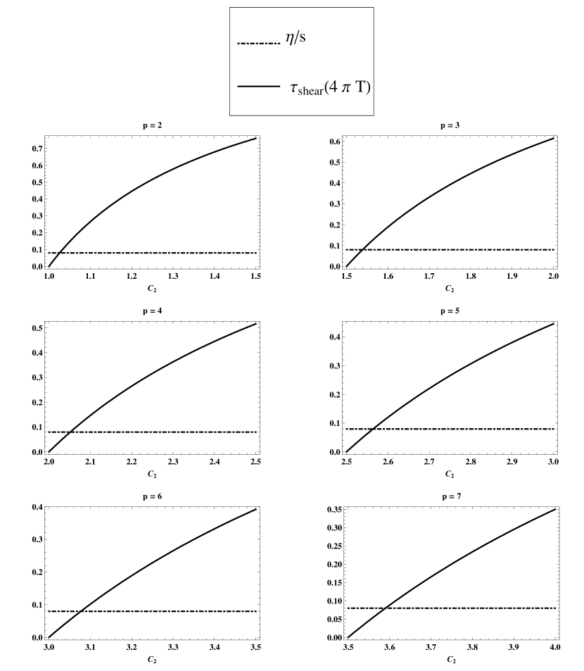
Figure 3: Plots of the dimensionless quantities: $\eta/s$ and $4\pi T\tau_{\rm shear}$, as a function of the free parameter $c_{2}$ appearing in the metric (194). Each plot corresponds to a different number of spatial dimensions $p$. This range of values of $c_{2}$ was chosen because outside this particular range, unphysical behavior is found in the sound mode. This will be explained in later chapters (cf. (289),(290)). The metric is conformal at the upper end of the range of $c_{2}$ when $c_{2}=(p+1)/2$. Note the universality of the shear viscosity to entropy density ratio is evident, while the value of $\tau_{\rm shear}$ varies with both $c_{2}$ and $p$.

Two notable special metrics are the Schwarzschild anti-de Sitter black hole, and the Dp-brane metric. The first of these is a black brane type metric which is a solution to Einstein’s equations with a negative cosmological constant. This ($p+2$ dimensional) metric can be written

$$ds^{2}_{SAdS} = \frac{r^{2}}{L^{2}}\left[-f(r)dt^{2}+dx_{j}dx^{j}\right]+\frac{L^{2}dr^{2}}{r^{2}f(r)}$$ (197)

$$f(r) = 1-\left(\frac{r_{0}}{r}\right)^{p+1}.$$ (198)

Here, $L$ is the usual $AdS$ curvature radius. Clearly, this fits the constraint (194) with $c_{2}=(p+1)/2$, thus for this metric we have

$$\tau_{\rm shear}^{SAdS}=\frac{1}{4\pi T}H_{n}\left(\frac{2}{p+1}\right).$$ (199)

As a second example, the Dp-brane metric arises from a stack of $N$ Dp-branes in string theory with $N\gg 1$. The metric exists in 10 dimensions, but can be reduced to an effective (p+2 dimensional) metric using dimensional reduction [47, 101]. The effective metric is a solution to Einstein’s equations where the metric is supported by a single scalar field, and the scalar potential is a single exponential

$$U(\phi)=-\frac{(7-p)(9-p)}{2L^{2}}e^{-\sqrt{\frac{2(3-p)^{2}}{p(9-p)}}\phi}.$$ (200)

The metric is:

$$ds^{2} = \left(\frac{r}{L}\right)^{\frac{9-p}{p}}\left[-f(r)dt^{2}+dx_{j}dx^{j}\right]+\left(\frac{r}{L}\right)^{\frac{p^{2}-8p+9}{p}}\frac{dr^{2}}{f(r)},$$ (201)

$$f(r) = 1-\left(\frac{r_{0}}{r}\right)^{7-p}.$$ (202)

This fits our special class of metrics with $c_{2}=(7p-p^{2})/(9-p)$. (Note that $p\leq 7$, or else the metric is not asymptotically anti-de Sitter.) Applying the formula (193) we have

$$\tau_{\rm shear}^{DP}=\frac{1}{4\pi T}H_{n}\left(\frac{5-p}{7-p}\right).$$ (203)

The results (199) and (203) were first presented by Natsuume in [105]. A few comments are in order about these applications. First, before the formula (193) was presented in [1], the quantity $\tau_{\rm shear}$ had been computed in several special cases, most notably in [89, 90]. The applications above (199) and (203) reproduce all known results in the literature, which is another check on our calculations. In addition, the formulas above give new information. A particularly curious feature is that $\tau_{\rm shear}^{Dp}=0$ for $p=5$, and $\tau_{\rm shear}^{Dp}\rightarrow\infty$ for $p>5$. It has been known that the Dp-brane metric exhibits unusual features for $p>4$ in the sound channel. (For example, for $p=5$, the speed of sound vanishes, while for $p>5$ the speed of sound becomes imaginary [101]). The analysis given here shows that these features are also present for the shear mode.

Furthermore, once we have completed the analysis of the sound mode, the comparison with the formula (195) gives us some information about the third order hydrodynamic contribution to the shear mode as mentioned in Sec. 5.3. This will be explained further in the next chapter.

Finally, perhaps the most obvious feature of these applications is that the quantity $\tau_{\rm shear}$ is not universal in the same way as the shear viscosity; application of the formula to different metrics yields different results.

14 Summary

In this chapter, we have applied the prescription which was outlined in Sec. 6 to shear perturbations of a black brane background supported by scalar fields. We have thus been able to determine the shear mode dispersion relation $w(q)$ up to order $q^{4}$. This dispersion relation is parametrized in (119) with two unknown quantities which we denote $D_{\eta}$ and $\tau_{\rm shear}$. The formulas (187) and (193) are the main results of this chapter, and they allow one to compute these unknown quantities if the background metric is given.

The formula for $D_{\eta}$, which was first derived in [47], allows one to compute the shear viscosity, since it is the only hydrodynamic transport coefficient which appears to lowest order in the shear dispersion relation. Application of the formula for $D_{\eta}$ to any Einstein gravity dual (in the limit of infinite coupling) yields $\eta/s=1/4\pi$, and is one of the main inspirations for the conjectured shear viscosity bound. The quantity $\tau_{\rm shear}$ does not display the same universal behavior.

It is important to make a distinction between the dispersion relation and the hydrodynamic transport coefficients which would appear in the derivative expansion of the energy momentum tensor. To lowest order, the shear dispersion relation contains only the shear viscosity, but at the next order ($q^{4}$), the quantity which we call $\tau_{\rm shear}$ contains more than one transport coefficient. (In fact, it contains contributions from third order hydrodynamics as explained in section 5.3). At this point, all we can state is that the combination of transport coefficients which comprise $\tau_{\rm shear}$ is not universal in the same way as the shear viscosity. If and when a consistent theory of third order hydrodynamics is formulated, one could revisit these results to see whether additional information about these new transport coefficients can be gained from the formula (193).

Chapter Sound Mode

15 Introduction

In this chapter, we will perform an analysis similar to that of the previous chapter within the context of a different hydrodynamic mode, the sound mode. In general, the prescription detailed in Sec. 6 will be applied in exactly the same way, but analysis is more complicated here due to the fact that the matter perturbations are coupled with the metric perturbations.

In [47], a formula for the shear viscosity to entropy density ratio $\eta/s$ was derived which is applicable to a wide variety of gravity duals. Application of this formula to known Einstein gravity duals always resulted in $\eta/s=1/4\pi$ (in the large N/infinite t’Hooft coupling limit), and eventually led to the celebrated viscosity bound conjecture that $\eta/s\geq 1/4\pi$ for all physical substances. Clearly, a similar general formula for the bulk viscosity would also be desirable in the hopes that other universal behavior might be discovered. Such a formula would also be useful when comparing the predictions of a phenomenological gravity dual to the lattice data [123, 124].

The work detailed in this chapter is partially motivated by the goal of obtaining such a formula, though such a formula has not yet been developed. This work should be viewed as a first step towards this goal. Here, we consider sound mode fluctuations of a dual gravity theory supported by a single scalar field, and then generalize to the case of multiple scalar fields. We attempt to be as general as possible by not specifying the background profiles of the scalar field(s) except in certain special cases.

Recent works [37, 125] also explore the sound mode in phenomenologically motivated single scalar models. The results presented here are complementary to these papers, though we allow for the possibility of multiple scalar fields, and also do not restrict ourselves to five dimensions.

The main results of this chapter are twofold. First, we derive a set of sound mode gauge invariant equations which are applicable to any Einstein gravity dual which is supported by $r$ dependent scalar fields. These equations are, in general, complicated but could be solved numerically to determine the sound mode dispersion relation for certain phenomenological models of the quark-gluon plasma. Second, we solve these equations analytically for the sound mode dispersion relation (up to order $q^{3}$) for a certain special class of metrics.

16 Background field and potential

We again work with the same set up as in the previous chapter. We will examine sound mode perturbations of a general black brane metric (23) with presumed near horizon behavior (24 - 26). We assume that the matter supporting the metric is scalar in nature, so that the action, background equations, and energy momentum tensor are given respectively by (120),(122), and (123).

Because the sound mode perturbations transform like scalars under rotations (see Sec. 5.2), the perturbations of the scalar fields will be coupled to the metric perturbations. For this reason, the sound mode requires more information about the matter perturbations than the shear mode. In particular, we will need information about the scalar potential.

The background equations of motion give a relationship between the scalar field profile and the potential.

$$\frac{\partial U(\phi_{i}(r))}{\partial\phi_{i}}=\Box^{(0)}\phi_{i}(r)=\frac{1}{\sqrt{-g}}\partial_{r}\left[\sqrt{-g}g^{rr}\phi_{i}^{\prime}(r)\right].$$ (204)

As usual, the prime denotes derivative with respect to $r$, and $\Box^{(0)}\equiv\nabla^{(0)}_{\mu}\nabla_{(0)}^{\mu}$. The covariant derivatives are defined in Appendix Hydrodynamics of Strongly Coupled Non-conformal Fluids from Gauge/Gravity Duality.

17 Perturbations and linearized equations

We now introduce fluctuations of the fields on this background $g_{\mu\nu}\rightarrow g_{\mu\nu}+h_{\mu\nu}$ and $\phi\rightarrow\phi+\delta\phi$, and assume the usual time dependence

$$h_{\mu\nu}(t,z,r) = e^{i(qz-wt)}h_{\mu\nu}(r),$$ (205)

$$\delta\phi(t,z,r) = e^{i(qz-wt)}\delta\phi(r).$$ (206)

The linearized Einstein equations for the sound mode and an arbitrary set of matter fields were derived in Sec. 6.3. In order to apply these equations to the case at hand, we must evaluate the perturbed energy momentum tensor for the case of the scalar fields. The energy momentum tensor was expanded to first order in the perturbation in (138). For the sound mode, we require the following components of the energy momentum tensor: $T^{tt},T^{aa},T^{zz},T^{tz},T^{rz},T^{tr},T^{rr}$. As in previous chapters, we use the subscripts (0) and (1) to distinguish background quantities from those that are $\mathcal{O}(h_{\mu\nu})$ or $\mathcal{O}(\delta\phi)$. A summation over the repeated index $k$, which labels the particular scalar field, is implied.

First, let us examine $T_{(1)}^{mn}$ with $m,n\neq r$. Using (138), we have

$$8\pi G_{p+2}T^{mn}_{(1)}=\frac{1}{2}\left(h^{mn}\mathcal{L}_{\phi}-g^{mn}\delta\mathcal{L}_{\phi}\right).$$ (207)

Noting that

$$16\pi G_{p+2}T^{mn}_{(0)}=-g^{mn}\mathcal{L}_{\phi},$$ (208)

and recalling the definitions of $A$,$B$,$C$, and $D$ (98)-(101) we have

$$16\pi G_{p+2}\left(T^{tt}_{(1)}+T^{tt}_{(0)}A\right) = -g^{tt}\delta\mathcal{L}_{\phi},$$ (209)

$$16\pi G_{p+2}\left(\frac{1}{p-1}\sum_{a=1}^{p-1}T^{aa}_{(1)}+T^{zz}_{(0)}B\right) = -g^{xx}\delta\mathcal{L}_{\phi},$$ (210)

$$16\pi G_{p+2}\left(T^{zz}_{(1)}+T^{zz}_{(0)}C\right) = -g^{xx}\delta\mathcal{L}_{\phi},$$ (211)

$$16\pi G_{p+2}\left(T^{tz}_{(1)}+T^{zz}_{(0)}D\right) = 0.$$ (212)

The right hand side is straightforward to evaluate

$$\delta\mathcal{L}_{\phi} = {\textstyle{\frac{1}{2}}}g^{\alpha\beta}\left[\partial_{\alpha}(\delta\phi_{k})\partial_{\beta}\phi_{k}+\partial_{\beta}(\delta\phi_{k})\partial_{\alpha}\phi_{k}\right]+\delta U$$ (213)

$$= \left(g^{rr}(\delta\phi_{k})^{\prime}\phi_{k}^{\prime}+\frac{\partial U}{\partial\phi_{k}}\delta\phi_{k}\right).$$

Secondly, examine $T_{(1)}^{mr}$:

$$8\pi G_{p+2}T^{mr}_{(1)}=\frac{1}{2}g^{mm}g^{rr}\partial_{m}(\delta\phi_{k})\partial_{r}\phi_{k},$$ (214)

This gives the relations

$$16\pi G_{p+2}T^{tr}_{(1)} = (-iw)g^{tt}g^{rr}(\delta\phi_{k})\phi_{k}^{\prime},$$ (215)

$$16\pi G_{p+2}T^{zr}_{(1)} = (iq)g^{xx}g^{rr}(\delta\phi_{k})\phi_{k}^{\prime}.$$ (216)

Finally, the only remaining component to evaluate is $T^{rr}_{(1)}$, evaluating (138) gives

$$8\pi G_{p+2}T^{rr}_{(1)}=\frac{1}{2}\left[2\left(g^{rr}\right)^{2}\partial_{r}(\delta\phi_{k})\partial_{r}\phi_{k}-g^{rr}\delta\mathcal{L}_{\phi}\right],$$ (217)

which simplifies to

$$16\pi G_{p+2}T^{rr}_{(1)}=(g^{rr})^{2}(\delta\phi_{k})^{\prime}\phi_{k}^{\prime}-g^{rr}\frac{\partial U}{\partial\phi_{k}}\delta\phi_{k}.$$ (218)

The insertion of these relations for the energy momentum tensor into the general sound mode equations (6.3 - 110) results in the following set of seven linearized Einstein equations. Here we have inserted a line above each equation that allows the reader to see which Einstein equation is the source of the following differential equation.

$G^{t\,(1)}_{\,t}=-8\pi G_{p+2}T^{t\,(1)}_{\,t}$

$$\frac{g_{rr}}{\sqrt{-g}}\sqrt{f}\partial_{r}\left[\frac{\sqrt{-g}g^{rr}}{\sqrt{f}}((p-1)B^{\prime}+C^{\prime})\right] + g_{rr}\frac{\partial U}{\partial\phi_{k}}(\delta\phi_{k})$$

$$+ \phi_{k}^{\prime}(\delta\phi_{k})^{\prime}-(p-1)q^{2}g_{rr}g^{xx}B=0,$$

$\displaystyle\sum_{i=1}^{p-1}G^{i\,(1)}_{\,i}=\displaystyle\sum_{i=1}^{p-1}\left(-8\pi G_{p+2}T^{i\,(1)}_{\,i}\right)$

$$\frac{g_{rr}}{\sqrt{-gf}}\partial_{r}\left[\sqrt{-gf}g^{rr}A^{\prime}\right] + \frac{g_{rr}}{\sqrt{-g}}\partial_{r}\left[\sqrt{-g}g^{rr}\left((p-2)B^{\prime}+C^{\prime}\right)\right]+g_{rr}\frac{\partial U}{\partial\phi_{k}}(\delta\phi_{k})$$

$$+\,\phi_{k}^{\prime}(\delta\phi_{k})^{\prime} - g_{rr}g^{xx}\left[q^{2}\left(A+(p-2)B\right)-\frac{w^{2}}{f}\left((p-2)B+C\right)+2qwD\right]$$ (220)

$$= 0\,$$

$G^{z\,(1)}_{\,z}=-8\pi G_{p+2}T^{z\,(1)}_{\,z}$

$$\frac{g_{rr}}{\sqrt{-gf}}\partial_{r}\left[\sqrt{-gf}g^{rr}A^{\prime}\right]+\frac{g_{rr}}{\sqrt{-g}}\partial_{r}\left[\sqrt{-g}g^{rr}(p-1)B^{\prime}\right] + g_{rr}\frac{\partial U}{\partial\phi_{k}}(\delta\phi_{k})+\phi_{k}^{\prime}(\delta\phi_{k})^{\prime}$$

$$- (p-1)w^{2}g_{rr}g^{tt}B=0,$$

(221)

$G^{z\,(1)}_{\,t}=-8\pi G_{p+2}T^{z\,(1)}_{\,t}$

$$\frac{\sqrt{-g}(g^{xx})^{p+1}}{f}\partial_{r}\left[\frac{(g_{xx})^{p+1}}{\sqrt{-g}}\partial_{r}\left(fD\right)\right]-2g_{rr}(F_{t}-F_{x})D+qw(p-1)g_{rr}g^{tt}B=0,$$

(222)

$G^{r\,(1)}_{\,r}=-8\pi G_{p+2}T^{r\,(1)}_{\,r}$

$$\mathcal{D}_{L}\left[(g_{xx})^{p}\right]A^{\prime}+\mathcal{D}_{L}\left[g_{tt}(g_{xx})^{p-1}\right]((p-1)B^{\prime}+C^{\prime})-2\phi_{k}^{\prime}(\delta\phi_{k})^{\prime}+2g_{rr}\frac{\partial U}{\partial\phi_{k}}(\delta\phi_{k})$$ (223)

$$-2g_{rr}\left(w^{2}g^{tt}((p-1)B+C)+q^{2}g^{xx}(A+(p-1)B)+2qwg^{xx}D\right) = 0,$$

$G^{t\,(1)}_{\,r}=-8\pi G_{p+2}T^{t\,(1)}_{\,r}$

$$w\sqrt{f}\partial_{r}\left[\frac{1}{\sqrt{f}}((p-1)B+C)\right]-qfD^{\prime}+w\phi_{k}^{\prime}(\delta\phi_{k})=0,$$ (224)

$G^{z\,(1)}_{\,r}=-8\pi G_{p+2}T^{z\,(1)}_{\,r}$

$$\frac{q}{\sqrt{f}}\partial_{r}\left[\sqrt{f}A\right]+\frac{w}{f}\partial_{r}\left[fD\right]+q(p-1)B^{\prime}+q\phi_{k}^{\prime}(\delta\phi_{k})=0.$$ (225)

In addition to these equations, one must also examine perturbations of the background scalar equations (204). Using the formulas given in the Appendix, especially (357) the equation for each scalar field (in the radial gauge, as usual) is

$\delta\left(\Box^{(0)}\phi_{i}\right)=\delta\left(\frac{\partial U}{\partial\phi_{i}}\right)$

$$\frac{g_{rr}}{\sqrt{-g}}\partial_{r}\left[\sqrt{-g}g^{rr}(\delta\phi_{i})^{\prime}\right]+{\textstyle{\frac{1}{2}}}\phi_{i}^{\prime}H^{\prime}-g_{rr}\left(w^{2}g^{tt}+q^{2}g^{xx}\right)(\delta\phi_{i})=g_{rr}\frac{\partial^{2}U}{\partial\phi_{i}\partial\phi_{k}}(\delta\phi_{k}).$$ (226)

Again, a summation over $k$ is implied and we have defined

$$H(r)\equiv A(r)+(p-1)B(r)+C(r).$$ (227)

18 Gauge Invariant Equations

There is still residual gauge freedom in these equations under the infinitesimal diffeomorphism (111). The scalar field perturbations also transform under a gauge transformation. Such a gauge transformation is essentially the freedom to choose ones coordinates. Imagine a small coordinate shift

$$x^{\mu}\rightarrow x^{\mu}-\xi^{\mu}.$$ (228)

Then, the background scalar field will be altered

$$\phi(x^{\mu})\rightarrow\phi(x^{\mu})-\xi^{\mu}\partial_{\mu}\phi(x^{\mu}).$$ (229)

The latter term appears to be a perturbation, but it is not a physical perturbation; it only appears due to a change in coordinates. Thus, under such a transformation, the scalar field perturbations behave as

$$\delta\phi_{i}\rightarrow\delta\phi_{i}-\xi^{\mu}\partial_{\mu}\phi_{i}=\delta\phi_{i}-\xi^{r}\phi_{i}^{\prime}.$$ (230)

Let us now examine how the different sound mode perturbations transform under this gauge transformation. Recall

$$\nabla^{(0)}_{\mu}\xi_{\nu}+\nabla^{(0)}_{\nu}\xi_{\mu}=\partial_{\mu}\xi_{\nu}+\partial_{\nu}\xi_{\mu}-2\Gamma^{\lambda}_{\mu\nu}\xi_{\lambda},$$ (231)

the Christoffel symbols given in Appendix Hydrodynamics of Strongly Coupled Non-conformal Fluids from Gauge/Gravity Duality, and the presumed form of the vector $\xi$ (112). Then, it is straightforward to evaluate

$$h_{tt} \rightarrow h_{tt}-2\partial_{t}\xi_{t}+2\Gamma_{tt}^{\lambda}\xi_{\lambda}=h_{tt}+2iw\xi_{t}-g^{rr}g_{tt}^{\prime}\xi_{r},$$ (232)

$$A \rightarrow A+2iwg^{tt}\xi_{t}-g^{rr}\mathcal{D}_{L}[g_{tt}]\xi_{r}.$$ (233)

In a similar manner,

$$B \rightarrow B-g^{rr}\mathcal{D}_{L}[g_{xx}]\xi_{r},$$ (234)

$$C \rightarrow C-2iqg^{xx}\xi_{z}-g^{rr}\mathcal{D}_{L}[g_{xx}]\xi_{r},$$ (235)

$$D \rightarrow D+iwg^{tt}\xi_{z}-iqg^{tt}\xi_{t}.$$ (236)

Given the transformation rules (230), (233), and (236), it is easy to verify that the following gauge invariant combinations first presented in [101] transform only into themselves under such a diffeomorphism (i.e. $Z_{0}\rightarrow Z_{0}$ and $Z_{\phi}\rightarrow Z_{\phi}$). The choice of these gauge invariant variables is not unique.

$$Z_{0}(r)=-f(r)\left[q^{2}A(r)+2qwD(r)\right]+w^{2}C(r)-\left[q^{2}\frac{g_{tt}^{\prime}(r)}{g_{xx}^{\prime}(r)}+w^{2}\right]B(r)$$ (237)

$$Z_{\phi i}(r)=\delta\phi_{i}(r)-\frac{\phi_{i}^{\prime}(r)}{\mathcal{D}_{L}\left[g_{xx}(r)\right]}B(r)$$ (238)

By taking an appropriate combination of the equations (17-226), one can arrive at coupled second order equations for the gauge invariant variables. Because of the complexity of the sound mode equations and the gauge invariant variables, reducing the linearized perturbation equations down to a set of gauge invariant equations is a very difficult task. The equations presented below were arrived at by “brute force”, by eliminating the variables $A,C,D,\delta\phi$ one at a time, and then by showing that the remaining coefficient of $B$ vanishes by the background equations of motion.

18.1 Equation for $Z_{0}$

First, define the quantity

$$\alpha(r)\equiv q^{2}\left((p-1)+\frac{\mathcal{D}_{L}[g_{tt}(r)]}{\mathcal{D}_{L}[g_{xx}(r)]}\right)-\frac{pw^{2}}{f(r)}.$$ (239)

Consider the following combination of the Einstein equations (17 - 226):

$$f \left\{\frac{\alpha}{p}\left[(\ref{g00scalareqn})-(\ref{gxxscalareqn})+(\ref{gzzscalareqn})+{\textstyle{\frac{1}{2}}}(\ref{grrscalareqn})\right]+\left[(\ref{g00scalareqn})+{\textstyle{\frac{1}{2}}}(\ref{grrscalareqn})\right]\left(\frac{w^{2}}{f}\right)-2qw(\ref{g0zscalareqn})\right.$$

$$- q^{2}\Biggl{.}\left[{\textstyle{\frac{1}{2}}}(\ref{grrscalareqn})+(\ref{gzzscalareqn})\right]\Biggr{\}}+2\left\{qf\mathcal{D}_{L}[\alpha](\ref{grzscalareqn})-w\mathcal{D}_{L}[\alpha f](\ref{g0rscalareqn})\right\}.$$

(240)

For simplicity, for the moment we assume there is only one scalar field. After a long calculation, one can show that this reduces to

$$\mathcal{Z}_{1}-2g_{rr}(F_{t}-F_{x})\left(w^{2}(B-C)+Z_{0}\right)-Bq^{2}f\Delta_{1}=0,$$ (241)

where

$$\mathcal{Z}_{1}\equiv\frac{g_{rr}}{\sqrt{-g}}\alpha^{2}f^{2}\partial_{r}\left[\frac{\sqrt{-g}g^{rr}}{\alpha^{2}f^{2}}Z_{0}^{\prime}\right]+Z_{0}\left(\mathcal{D}_{L}[f]\mathcal{D}_{L}[f\alpha]-g_{rr}\left(w^{2}g^{tt}+q^{2}g^{xx}\right)\right) +$$

$$2Z_{\phi}\phi^{\prime}f\left(\alpha\partial_{r}\left[\frac{1}{\alpha}\left(\frac{w^{2}}{f}-q^{2}\right)\right]+\frac{q^{2}\mathcal{D}_{L}[f]}{p\mathcal{D}_{L}[g_{xx}]}\mathcal{D}_{L}\left[\sqrt{-g}g^{rr}\phi^{\prime}\right]\right),$$ (242)

and

$$\Delta_{1} \equiv 2\mathcal{D}_{L}[g_{xx}]\alpha^{2}\partial_{r}\left[\frac{g_{rr}}{\alpha^{2}\mathcal{D}_{L}[g_{xx}]^{2}}(F_{t}-F_{x})\right]-\frac{4g_{rr}}{p\mathcal{D}_{L}[g_{xx}]^{2}}(F_{t}-F_{x})(\phi^{\prime})^{2}$$ (243)

$$+ \alpha^{2}\mathcal{D}_{L}[f]\partial_{r}\left[\frac{1}{p\alpha^{2}\mathcal{D}_{L}[g_{xx}]^{2}}\left(2g_{rr}(F_{t}-F_{r})-(\phi^{\prime})^{2}\right)\right].$$

Here, we have been able to eliminate the potential using (204), since it only appears in these equations via $\partial U/\partial\phi$. Clearly, $\Delta_{1}$ vanishes by the background equations of motion (130) and (128), leaving a differential equation involving only the gauge invariant variables, namely $\mathcal{Z}_{1}=0$,

$$\frac{g_{rr}}{\sqrt{-g}}\alpha^{2}f^{2}\partial_{r}\left[\frac{\sqrt{-g}g^{rr}}{\alpha^{2}f^{2}}Z_{0}^{\prime}\right]+Z_{0}\left(\mathcal{D}_{L}[f]\mathcal{D}_{L}[f\alpha]-g_{rr}\left(w^{2}g^{tt}+q^{2}g^{xx}\right)\right) +$$ (244)

$$2Z_{\phi}\phi^{\prime}f\left(\alpha\partial_{r}\left[\frac{1}{\alpha}\left(\frac{w^{2}}{f}-q^{2}\right)\right]+\frac{q^{2}\mathcal{D}_{L}[f]}{p\mathcal{D}_{L}[g_{xx}]}\mathcal{D}_{L}\left[\sqrt{-g}g^{rr}\phi^{\prime}\right]\right) = 0.$$

In this special case of one scalar field, one can write these equations only in terms of the metric components because of the relation (128).

The generalization to multiple scalar fields is straightforward. Since all of the equations used to derive (244) depend only on the sum of all scalar fields, it is clear that all we need to do is include a summation on the last term. An explicit calculation (using the same combination of background Einstein equations) reveals this is correct. The generalization is

$$\frac{g_{rr}}{\sqrt{-g}}\alpha^{2}f^{2}\partial_{r}\left[\frac{\sqrt{-g}g^{rr}}{\alpha^{2}f^{2}}Z_{0}^{\prime}\right]+Z_{0}\left(\mathcal{D}_{L}[f]\mathcal{D}_{L}[f\alpha]-g_{rr}\left(w^{2}g^{tt}+q^{2}g^{xx}\right)\right) +$$

$$\sum_{k=1}^{n}\left\{2Z_{\phi k}\phi_{k}^{\prime}f\left(\alpha\partial_{r}\left[\frac{1}{\alpha}\left(\frac{w^{2}}{f}-q^{2}\right)\right]+\frac{q^{2}\mathcal{D}_{L}[f]}{p\mathcal{D}_{L}[g_{xx}]}\mathcal{D}_{L}\left[\sqrt{-g}g^{rr}\phi_{k}^{\prime}\right]\right)\right\} = 0$$ (245)

18.2 Equations for $Z_{\phi i}$

We now proceed to derive the other gauge invariant equations. There will be an additional gauge invariant equation for each background scalar field present. The relevant combination of equations is:

$$(\ref{scalareqn}) + \frac{\phi_{i}^{\prime}}{p\mathcal{D}_{L}[g_{xx}]}\left\{(\ref{gxxscalareqn})-(\ref{gzzscalareqn})-(\ref{g00scalareqn})-\frac{1}{2}(\ref{grrscalareqn})\right\}$$ (246)

$$+ \frac{2}{\alpha}\partial_{r}\left[\frac{\phi_{i}^{\prime}}{\mathcal{D}_{L}[g_{xx}]}\right]\left\{\frac{w}{f}(\ref{g0rscalareqn})-q(\ref{grzscalareqn})\right\}.$$

Another lengthy calculation reduces this combination to

$$\mathcal{Z}_{2}-B\Delta_{2}=0,$$ (247)

where

$$\mathcal{Z}_{2} \equiv \frac{g_{rr}}{\sqrt{-g}}\partial_{r}\left[\sqrt{-g}g^{rr}Z_{\phi i}^{\prime}\right]-Z_{\phi i}g_{rr}\left(w^{2}g^{tt}+q^{2}g^{xx}\right)-g_{rr}\sum_{k=1}^{n}Z_{\phi k}\frac{\partial^{2}U}{\partial\phi_{i}\partial\phi_{k}}$$ (248)

$$- \frac{2\phi_{i}^{\prime}}{p\mathcal{D}_{L}[g_{xx}]\alpha}\left\{\sum_{k=1}^{n}\left[Z_{\phi k}\phi_{k}^{\prime}\left(\alpha\mathcal{D}_{L}\left[\sqrt{-g}g^{rr}\phi_{k}^{\prime}\right]+p\mathcal{D}_{L}\left[\frac{\phi_{i}^{\prime}}{\mathcal{D}_{L}[g_{xx}]}\right]\left(q^{2}-\frac{w^{2}}{f}\right)\right)\right]\right\}$$

$$+ \frac{2}{\alpha\sqrt{f}}\partial_{r}\left[\frac{\phi_{i}^{\prime}}{\mathcal{D}_{L}[g_{xx}]}\right]\partial_{r}\left[\frac{Z_{0}}{\sqrt{f}}\right],$$

and

$$\Delta_{2} \equiv \frac{g_{rr}}{\mathcal{D}_{L}[g_{xx}]}\left\{\sum_{k}\frac{\partial^{2}U}{\partial\phi_{i}\partial\phi_{k}}\phi_{k}^{\prime}-\partial_{r}\left[\frac{1}{\sqrt{-g}}\partial_{r}\left[\sqrt{-g}g^{rr}\phi_{i}^{\prime}\right]\right]\right\}$$ (249)

$$+ \frac{\phi_{i}^{\prime}}{p\mathcal{D}_{L}[g_{xx}]^{2}}\left(\frac{g_{rr}}{\sqrt{-g}}\right)^{2}\partial_{r}\left\{\left(\sqrt{-g}g^{rr}\right)^{2}\left[\sum_{k}(\phi_{k}^{\prime})^{2}-2g_{rr}(F_{t}-F_{r})\right]\right\}$$

$$+ \frac{2}{\alpha\mathcal{D}_{L}[g_{xx}]}\partial_{r}\left[\frac{\phi_{i}^{\prime}}{\mathcal{D}_{L}[g_{xx}]}\right]\left(\sum_{k}(\phi_{k}^{\prime})^{2}-2g_{rr}(F_{t}-F_{r})\right)\left(q^{2}-\frac{w^{2}}{f}\right)$$

$$+ \frac{2g_{rr}}{\mathcal{D}_{L}[g_{xx}]}\left(\frac{2q^{2}}{\alpha}\partial_{r}\left[\frac{\phi_{i}^{\prime}}{\mathcal{D}_{L}[g_{xx}]}\right]+\phi_{i}^{\prime}\right)(F_{t}-F_{x}).$$

Again, $\Delta_{2}$ vanishes by the background equations of motion (128), (130), and (204). Thus, we are left with an equation only containing the gauge invariant variables, $\mathcal{Z}_{2}=0$:

$$\frac{g_{rr}}{\sqrt{-g}}\partial_{r}\left[\sqrt{-g}g^{rr}Z_{\phi i}^{\prime}\right]-Z_{\phi i}g_{rr}\left(w^{2}g^{tt}+q^{2}g^{xx}\right)-g_{rr}\sum_{k=1}^{n}Z_{\phi k}\frac{\partial^{2}U}{\partial\phi_{i}\partial\phi_{k}}$$ (250)

$$- \frac{2\phi_{i}^{\prime}}{p\mathcal{D}_{L}[g_{xx}]\alpha}\left\{\sum_{k=1}^{n}\left[Z_{\phi k}\phi_{k}^{\prime}\left(\alpha\mathcal{D}_{L}\left[\sqrt{-g}g^{rr}\phi_{k}^{\prime}\right]+\mathcal{D}_{L}\left[\frac{\phi_{i}^{\prime}}{\mathcal{D}_{L}[g_{xx}]}\right]\left(q^{2}-\frac{w^{2}}{f}\right)\right)\right]\right\}$$

$$+ \frac{2}{\alpha\sqrt{f}}\partial_{r}\left[\frac{\phi_{i}^{\prime}}{\mathcal{D}_{L}[g_{xx}]}\right]\partial_{r}\left[\frac{Z_{0}}{\sqrt{f}}\right]=0.$$

When only one scalar field is present, (250) simplifies. This equation contains the combination $\partial^{2}U/\partial\phi_{i}\partial\phi_{k}$. In the case of one scalar field, one can use

$$\frac{d^{2}U(\phi(r))}{d\phi^{2}}=\frac{1}{\phi^{\prime}(r)}\partial_{r}\left[\frac{dU(\phi(r))}{d\phi}\right],$$ (251)

which, along with the expression for $U^{\prime}(\phi)$ (204), allows us to eliminate the potential completely in favor of the field $\phi$.

$$\frac{g_{rr}}{\sqrt{-g}}\partial_{r}\left[\sqrt{-g}g^{rr}Z_{\phi}^{\prime}\right]+\frac{2}{\alpha}\partial_{r}\left[\frac{\phi^{\prime}}{\mathcal{D}_{L}[g_{xx}]}\right]\left\{\frac{1}{\sqrt{f}}\partial_{r}\left[\frac{Z_{0}}{\sqrt{f}}\right]-\left(q^{2}-\frac{w^{2}}{f}\right)\phi^{\prime}Z_{\phi}\right\}$$ (252)

$$-Z_{\phi}\left\{g_{rr}\left(q^{2}g^{xx}+w^{2}g^{tt}\right)+\frac{\left(\mathcal{D}_{L}[g_{xx}]\right)^{2}}{f\phi^{\prime}}\partial_{r}\left[\frac{f\phi^{\prime}}{\left(\mathcal{D}_{L}[g_{xx}]\right)^{2}}\mathcal{D}_{L}\left[\sqrt{-g}g^{rr}\phi^{\prime}\right]\right]\right\} = 0$$

The equations (18.1) and (250) are the most general gauge invariant equations for any black brane background supported by $r$ dependent scalar fields. If only one scalar field is present, one can use (244) and (252). To determine the dispersion relation, one needs to solve the above equations perturbatively in $w,q$ as explained in previous chapters. Some terms can be neglected when considering these equations to $\mathcal{O}(w,q)$, but one should keep in mind that $Z_{0}$ is $\mathcal{O}(q^{2})$, $Z_{\phi}$ is $\mathcal{O}(1)$, and $\alpha$ is $\mathcal{O}(q^{2})$.

19 Special case solution

19.1 Solution for $Z_{\phi}$

Even for the case of a single scalar field, the gauge invariant equations are quite complicated and we have been unable to find a general analytic solution. However, analytic solutions do exist for certain special backgrounds, as we now show.

Consider the special case of one scalar field with profile $\phi(r)=\kappa\log\left[g_{xx}(r)\right]+\phi_{0}$ where $\kappa$ and $\phi_{0}$ are constants. In this special case, the equation (252) reduces to

$$\frac{g_{rr}}{\sqrt{-g}}\partial_{r}\left[\sqrt{-g}g^{rr}Z_{\phi}^{\prime}\right]-Z_{\phi}g_{rr}\left(q^{2}g^{xx}+w^{2}g^{tt}\right)=0.$$ (253)

This can be more easily seen by re-writing

$$\partial_{r}\left[\frac{f\phi^{\prime}}{\left(\mathcal{D}_{L}[g_{xx}]\right)^{2}}\mathcal{D}_{L}\left[\sqrt{-g}g^{rr}\phi^{\prime}\right]\right]$$ (254)

$$= \kappa\,\partial_{r}\left[\frac{f}{\mathcal{D}_{L}[g_{xx}]}\mathcal{D}_{L}\left[\sqrt{-g}g^{rr}\mathcal{D}_{L}[g_{xx}]\right]\right]$$ (255)

$$= \kappa\left\{\frac{2g_{rr}f}{\mathcal{D}_{L}[g_{xx}]}(F_{t}-F_{x})-f\partial_{r}\left[\frac{2g_{rr}(F_{t}-F_{r})}{p\left(\mathcal{D}_{L}[g_{xx}]\right)^{2}}\right]\right\}$$ (256)

$$= \kappa\left\{\frac{2g_{rr}f}{\mathcal{D}_{L}[g_{xx}]}(F_{t}-F_{x})-f\partial_{r}\left[\frac{\phi^{\prime}(r)^{2}}{p\left(\mathcal{D}_{L}[g_{xx}]\right)^{2}}\right]\right\}$$ (257)

$$= 0,$$ (258)

where we have used (128) and (130) in the last two steps.

We now proceed according to the prescription outlined in Chapter Hydrodynamics of Strongly Coupled Non-conformal Fluids from Gauge/Gravity Duality by applying the incoming wave ansatz

$$Z_{0}(r) = f(r)^{-\frac{iw}{4\pi T}}\left(Y_{0}(r)+qY_{1}(r)+...\right)$$ (259)

$$Z_{\phi}(r) = f(r)^{-\frac{iw}{4\pi T}}\left(Y_{\phi 0}(r)+qY_{\phi 1}(r)+...\right)$$ (260)

$$w(q) = w_{1}q+w_{2}q^{2}+w_{3}q^{3}+...$$ (261)

with the condition that all $Y$ functions are regular at the horizon. Inserting this ansatz into (253), and expanding the result in powers of q, we have the following equation which is good up to $\mathcal{O}(q^{2})$:

$$\partial_{r}\left[\sqrt{-g}g^{rr}Y_{\phi 0}^{\prime}\right]+q\,\partial_{r}\left[\sqrt{-g}g^{rr}\left(Y_{\phi 1}^{\prime}-\frac{iw_{1}}{2\pi T}\mathcal{D}_{L}(f)Y_{\phi 0}\right)\right].$$ (262)

It should be noted that we have omitted some terms which are proportional to ($R^{0}_{0}-R^{x}_{x}$) since they vanish by the background equations of motion. Solving this order by order in $q$ is now quite simple. The solution for $Y_{\phi 0}$ can be written in terms of an integral

$$Y_{\phi 0}(r)=c_{0}+c_{1}\int_{r}^{\infty}\frac{g_{rr}(r^{\prime})}{\sqrt{-g(r^{\prime})}}dr^{\prime},$$ (263)

but this integral is logarithmically divergent at the horizon by (25). Thus, the assumption of regularity on the $Y$ functions leads to $Y_{\phi 0}=c_{0}$. Finally, this constant must be set to zero by the Dirichlet boundary condition at infinity. Plugging $Y_{\phi 0}=0$ into the next order equation, one also finds $Y_{\phi 1}=0$. Proceeding now to higher orders in $q$, one finds that the equations always reduce to the same as that for $Y_{0}$, and as a result $Z_{\phi}=0$ to all orders in $q$. With this simplification, the gauge invariant equation for $Z_{0}$ that must be solved is

$$\frac{g_{rr}}{\sqrt{-g}}\alpha^{2}f^{2}\partial_{r}\left[\frac{\sqrt{-g}g^{rr}}{\alpha^{2}f^{2}}Z_{0}^{\prime}\right]+Z_{0}\left\{\mathcal{D}_{L}[f]\mathcal{D}_{L}[f\alpha]-g_{rr}\left(w^{2}g^{tt}+q^{2}g^{xx}\right)\right\} = 0$$

(264)

19.2 Constraints on the metric and scalar potential

Next, one must solve the equation for $Z_{0}$ using these boundary conditions with the knowledge that $Z_{\phi}=0$. Before doing so, it is useful to pause and ask what type of metrics these results will be applicable to. There are three unknown metric functions, $g_{tt},g_{xx}$, and $g_{rr}$, but we have two constraints on them, namely (128) and (130). These two equations allow one to solve for both $g_{tt}$ and $g_{rr}$ in terms of $g_{xx}$. Solving (130) gives $g_{rr}$ in terms of the other metric components and one integration constant $c_{1}$,

$$g_{rr}(r)=c_{1}g_{xx}(r)^{p+1}f(r)\mathcal{D}_{L}[f(r)]^{2}.$$ (265)

For convenience, we define the constant of proportionality between $\phi(r)$ and $\log[g_{xx}]$ as

$$\phi(r) = \kappa\log[g_{xx}(r)]+\phi_{0}$$ (266)

$$\kappa \equiv \pm\sqrt{\frac{p}{2}\left(p+1-2c_{2}\right)}.$$ (267)

where $\phi_{0}$ is an integration constant.

Taking this solution, plugging into (128) and solving for $g_{tt}$ gives $f(r)$ in terms of $g_{xx}$ and three constants $c_{2}$, $c_{3}$ and $c_{4}$. These constants could in principle depend on $r_{0}$, but are independent of $r$,

$$f(r)=c_{3}\left[1-c_{4}\left(\frac{1}{g_{xx}(r)}\right)^{c_{2}}\right].$$ (268)

Imposing the requirement that the function $f$ must vanish at the horizon determines $c_{4}$. Furthermore let us assume that the metric is asymptotically $AdS$, so that for $r\to\infty$, $g_{xx}(r)\propto r^{n}$. Where $n$ is some positive exponent. Then we must have $c_{3}=1$, and $c_{2}>0$ for the correct asymptotic behavior of $f$. This determines $f$ up to a single constant,

$$f(r)=1-\left(\frac{g_{xx}(r_{0})}{g_{xx}(r)}\right)^{c_{2}}.$$ (269)

which is exactly the same metric constraint we considered previously (194). In the previous chapter, we simply imposed this constraint by hand. Here we have shown that the constraint arises naturally by first imposing a particular condition on the scalar field which simplifies the gauge invariant equations. The Hawking temperature for this metric can be found from (39) as

$$\frac{1}{(4\pi T)^{2}}=c_{1}g_{xx}(r_{0})^{p}.$$ (270)

It is also interesting to ask what sort of scalar potential can generate such a metric. One can determine the form of the potential by considering the following combination of background Einstein equations

$$g^{tt}G^{(0)}_{tt}+g^{rr}G^{(0)}_{rr}=-8\pi G_{p+2}\left(g^{tt}T^{(0)}_{tt}+g^{rr}T^{(0)}_{rr}\right)=U(\phi).$$ (271)

An explicit computation of the left hand side for our special metric gives

$$U(\phi(r))=-\frac{p}{2c_{1}\,c_{2}}g_{xx}(r_{0})^{-2c_{2}}g_{xx}(r)^{-\frac{2}{p}\kappa^{2}}.$$ (272)

Using (266), we find

$$U(\phi)=-\frac{p}{2c_{1}c_{2}}g_{xx}(r_{0})^{-2c_{2}}\exp\left(-\frac{2}{p}\kappa(\phi-\phi_{0})\right).$$ (273)

Thus, the sort of metrics we are considering are those generated by a potential which contains a single exponential, similar to the Chamblin-Reall backgrounds [126] examined in [36, 125]. It is amusing that we have arrived at the same metric considered in these references, as our only guiding principle has been to search for a class of metrics which simplify the gauge invariant equations (244),(252).

Finally, note that since the potential must be independent of temperature, it is required that the constant $c_{2}$, and the combination $c_{1}g_{xx}(r_{0})^{2c_{2}}$ must themselves be independent of $r_{0}$.

19.3 First order hydrodynamics

One must now go back to (244), insert $Z_{\phi}=0$ and the incoming wave ansatz (261), and expand the resulting equation in powers of $q$. In doing so, one should take into account the constraints (265) and (269). The first of these constraints allows one to eliminate $\sqrt{-g}g^{rr}$ in favor of $\mathcal{D}_{L}[f]$. Once this is done, the lowest order equation for $Y_{0}$ can be written

$$\frac{\left(C_{0}-f(p-c_{2})\right)^{2}}{(p-c_{2})f}\partial_{r}\left[\frac{1}{\mathcal{D}_{L}[f]\left(C_{0}-f(p-c_{2})\right)^{2}}Y_{0}^{\prime}\right]-\frac{\mathcal{D}_{L}[f]}{C_{0}-f(p-c_{2})}Y_{0}=0,$$ (274)

where

$$C_{0}\equiv pw_{1}^{2}-c_{2}.$$ (275)

The general solution to that equation contains two arbitrary constants $k_{1}$ and $k_{2}$, and can be written

$$Y_{0}(r)=[pw_{1}^{2}-c_{2}+f(r)(p-c_{2})]\left[k_{0}+k_{1}\int_{r}^{\infty}\,\left(\frac{pw_{1}^{2}-c_{2}-(p-c_{2})f(r^{\prime})^{2}}{pw_{1}^{2}-c_{2}+(p-c_{2})f(r^{\prime})^{2}}\right)^{2}\frac{f^{\prime}(r^{\prime})}{f(r^{\prime})}\,dr^{\prime}\right],$$ (276)

as can be found by first making the ansatz $Y_{0}(r)=b_{0}+b_{1}f(r)$, and then using the technique of reduction of order once this solution is found (cf. Appendix Hydrodynamics of Strongly Coupled Non-conformal Fluids from Gauge/Gravity Duality). The integral in (276) is logarithmically divergent near the horizon, and thus the requirement of regularity leads to $k_{1}=0$. Finally, applying the Dirichlet boundary condition at $r\rightarrow\infty$, leads to

$$w_{1}^{2}=\frac{2c_{2}}{p}-1,$$ (277)

where we have assumed that $f(r\rightarrow\infty)=1$.

Proceeding now to the next order in $q$, and substituting the solutions for $w_{1}$ and $Y_{0}$, one finds the following differential equation for $Y_{1}$:

$$\partial_{r}\left[\frac{Y_{1}^{\prime}}{\mathcal{D}_{L}[f](1+f)^{2}}\right]+\frac{f^{\prime}}{(1+f)^{3}}\left[Y_{1}-w_{1}k_{0}\left(\frac{i(p-c_{2})}{\pi T}+2pw_{2}\right)\right]=0.$$ (278)

The solution to the homogeneous part can be found using the same techniques as for the solution for $Y_{0}$ listed above. A particular solution to the inhomogeneous equation is obviously $Y_{1}(r)=\,$Constant. This leads to the general solution,

$$Y_{1}(r)=(f(r)-1)\left(k_{2}+k_{3}\int_{r}^{\infty}\frac{(f(r^{\prime})+1)^{2}}{(f(r^{\prime})-1)^{2}}\frac{f^{\prime}(r^{\prime})}{f(r^{\prime})}\,dr^{\prime}\right)+w_{1}k_{0}\left(\frac{i(p-c_{2})}{\pi T}+2pw_{2}\right).$$ (279)

The integral above is again logarithmically divergent, leading to the requirement that $k_{3}=0$. Applying now the Dirichlet boundary condition at $r\rightarrow\infty$ leads to

$$w_{1}k_{0}\left(\frac{i(p-c_{2})}{\pi T}+2pw_{2}\right)=0,$$ (280)

$$w_{2}=\frac{i(c_{2}-p)}{2\pi Tp}.$$ (281)

Note that we require $c_{2}<p$ to avoid exponential growth of the perturbations. Let us summarize the central results of this section:

$$Y_{0}(r) = y_{0}\left(f(r)-1\right),$$ (282)

$$Y_{1}(r) = y_{1}\left(f(r)-1\right),$$ (283)

$$w_{1} = \pm\sqrt{\frac{2c_{2}}{p}-1},$$ (284)

$$w_{2} = -\frac{i(p-c_{2})}{2\pi Tp}.$$ (285)

Here $y_{0}=k_{0}(c_{2}-p)$ is a constant, though its value is unimportant as it does not enter into any formulas for physical quantities, and we have relabeled $k_{2}$ as $y_{1}$ for aesthetic reasons.

Comparing these results to the dispersion relation expected from first order hydrodynamics (72)

$$w_{1} = \pm v_{s},$$ (286)

$$w_{2} = -i\frac{\eta}{\epsilon+P}\left(\frac{p-1}{p}+\frac{\zeta}{2\eta}\right),$$ (287)

one gains knowledge of $v_{s}$ (speed of sound), $\eta$ (shear viscosity), and $\zeta$ (bulk viscosity):

$$\eta/s = 1/4\pi,$$ (288)

$$v_{s} = \sqrt{\frac{2c_{2}}{p}-1},$$ (289)

$$\zeta/\eta = 2\left(\frac{1}{p}-v_{s}^{2}\right).$$ (290)

Here we remind the reader that $s=(\epsilon+P)/T$ is the entropy density, $\epsilon$ is the equilibrium energy density, and $P$ is the equilibrium pressure. Note that the conjectured bulk viscosity bound of Buchel [127] is saturated for metrics of this type.

19.4 Digression: comparison with black hole thermodynamics

It is interesting to note that the speed of sound can be derived solely from the metric by using relations from black hole thermodynamics. Such a formula was derived in Chapter Hydrodynamics of Strongly Coupled Non-conformal Fluids from Gauge/Gravity Duality, (cf. 45). Applying it to the special metric and using (39) and (270) results in

$$v_{s}^{2}=-\frac{1}{p}\left[p+\frac{\frac{d}{dr_{0}}Log[c_{1}]}{\frac{d}{dr_{0}}Log[g_{xx}(r_{0})]}\right].$$ (291)

Recall that $c_{1}$ is independent of $r$, but could in principle depend on $r_{0}$. At first sight this seems quite puzzling due to the presence of the constant $c_{1}$ which is not present in the formula (289). These two calculations of the speed of sound must agree.

The resolution of this apparent contradiction lies in the observation made at the end of Sec. (19.2). In order to have a sensible potential which is temperature independent, both $c_{2}$ and $c_{1}g_{xx}(r_{0})^{2c_{2}}$ must be independent of temperature (and thus also independent of $r_{0}$). As a result, we have

$$c_{1}\propto g_{xx}(r_{0})^{-2c_{2}},$$ (292)

where the constant of proportionality is independent of $r$ and $r_{0}$. Substituting this into (291) provides

$$v_{s}^{2}=\frac{2c_{2}}{p}-1,$$ (293)

which is exactly the same as that computed from the gravitational perturbations. It is quite reassuring that these two calculations agree. It is interesting that this latter method is much more efficient for computing the speed of sound; unfortunately, it does not give access to the bulk viscosity and any higher order transport coefficients.

19.5 Second order hydrodynamics

It is the purpose of this section to extend the above calculation to the next hydrodynamic order, and thus to determine the next coefficient in the dispersion relation $w_{3}$.

19.5.1 Equation for $Y_{2}$

We have already shown that $Z_{\phi}$ vanishes to all orders in $q$, so then it remains to return to (19.1), insert the incoming wave ansatz, expand in powers of $q$, and insert the solutions (282 - 285). Completing these steps, one finds the following differential equation which must be solved for $Y_{2}$:

$$\partial_{r}\left[\frac{Y_{2}^{\prime}}{\mathcal{D}_{L}[f](1+f)^{2}}\right]+$$

$$\frac{f^{\prime}}{(1+f)^{3}}\left\{Y_{2}+\frac{y_{0}}{(4\pi T)^{2}}\left[x_{0}+\frac{1-f^{2}}{f}\left(w_{1}^{2}+\frac{g_{xx}(r)^{p}}{g_{xx}(r_{0})^{p}}\left(f-w_{1}^{2}\right)\right)\right]\right\}=0,$$

where

$$x_{0}\equiv 2\left(5w_{1}^{2}-1-\frac{2w_{1}w_{3}(4\pi T)^{2}}{1-w_{1}^{2}}\right).$$ (295)

In writing the above expression, we have replaced all occurrences of the constant $c_{2}$ which appears in the metric with $w_{1}$ due to the relation (284), and have removed the constant $c_{1}$ in favor of $T$ using (270).

19.5.2 Solution for $Y_{2}$

The associated homogeneous equation for (19.5.1) is the same as the homogeneous part of the equation for $Y_{1}$, (278). The solution can easily be found by first making the ansatz $Y_{2}(r)=y_{2a}(1-f(r))$, and then using the technique of reduction of order once this solution is found. The general solution to the homogeneous part of the above equation is

$$Y_{2h}(r)=y_{2a}(1-f(r))+y_{2b}\Bigl{[}(1-f(r))\log[f(r)]+4\Bigr{]}.$$ (296)

Here the subscript $h$ stands for homogeneous, and $y_{2a}$, $y_{2b}$ are arbitrary constants.

In order to find the general solution for $Y_{2}$, we must now find a particular solution to the inhomogeneous equation. Since the homogeneous solution is known, one can construct a particular solution using the method of variation of parameters. For completeness, this method is outlined in Appendix G. Using the notation from Appendix G, (and changing independent variables from $x$ to $r$), we have

$$y_{1}(r) = 1-f(r),$$ (297)

$$h(r) = \log[f(r)]+\frac{4}{1-f(r)},$$ (298)

$$g(r) = -\frac{(f^{\prime})^{2}}{f(1+f)}\frac{y_{0}}{(4\pi T)^{2}}\left[x_{0}+\frac{1-f^{2}}{f}\left(w_{1}^{2}+\frac{g_{xx}(r)^{p}}{g_{xx}(r_{0})^{p}}\left(f-w_{1}^{2}\right)\right)\right].$$ (299)

After some simplification, one can write the particular solution as,

$$Y_{2p}(r) = -\frac{y_{0}}{(4\pi T)^{2}}(1-f(r))\left[\int\left(\frac{1+f(r)}{1-f(r)}\right)^{2}\frac{f^{\prime}(r)}{f(r)}Q(r)\,dr\right]$$ (300)

$$Q(r) = \int^{r}\frac{(1-f(z))}{(1+f(z))^{3}}f^{\prime}(z)\left[x_{0}+\frac{1-f(z)^{2}}{f(z)}\left(w_{1}^{2}+\frac{g_{xx}(z)^{p}}{g_{xx}(r_{0})^{p}}\left(f(z)-w_{1}^{2}\right)\right)\right]\,dz.$$

(301)

The term involving $x_{0}$ can be integrated directly, by changing variables from $z$ to $f$. This simplifies the solution to

$$Y_{2p}(r)=-\frac{x_{0}y_{0}}{(4\pi T)^{2}}+\frac{y_{0}}{(4\pi T)^{2}}(f(r)-1)\left[\int\left(\frac{1+f(r)}{1-f(r)}\right)^{2}\frac{f^{\prime}(r)}{f(r)}\hat{Q}(r)\,dr\right],$$ (302)

$$\hat{Q}(r)=\int^{r}\left(\frac{1-f(\tilde{r})}{1+f(\tilde{r})}\right)^{2}\frac{f^{\prime}(\tilde{r})}{f(\tilde{r})}\left[w_{1}^{2}+\frac{g_{xx}(\tilde{r})^{p}}{g_{xx}(r_{0})^{p}}\left(f(\tilde{r})-w_{1}^{2}\right)\right]\,d\tilde{r},$$ (303)

and so, the general solution for $Y_{2}$ is given by

$$Y_{2}(r)=Y_{2h}(r)+Y_{2p}(r).$$ (304)

To proceed, it is convenient to change coordinates. We define the coordinate $u$ by

$$u^{2}\equiv\left(\frac{g_{xx}(r_{0})}{g_{xx}(r)}\right)^{c_{2}}=\left(\frac{g_{xx}(r_{0})}{g_{xx}(r)}\right)^{\frac{p}{2}(w_{1}^{2}+1)},$$ (305)

so that

$$f(u)=1-u^{2},$$ (306)

and the horizon is now located at $u=1$, and the boundary is located at $u=0$.In terms of the new coordinates, $Y_{2}$ is given by

$$Y_{2h}(u)=y_{2a}u^{2}+y_{2b}\Bigl{[}u^{2}\log[1-u^{2}]+4\Bigr{]},$$ (307)

$$Y_{2p}(u)=-\frac{y_{0}}{(4\pi T)^{2}}\Biggl{\{}x_{0}+4u^{2}\int\frac{(2-u^{2})^{2}}{u^{3}(1-u^{2})}\int^{u}\frac{v^{5}\left[w_{1}^{2}+v^{-4/(1+w_{1}^{2})}\left(1-v^{2}-w_{1}^{2}\right)\right]}{(2-v^{2})^{2}(1-v^{2})}\,dv\,du\Biggr{\}}$$ (308)

The inner integral in this latter equation can be written in terms of hypergeometric functions, but the result is not particularly enlightening, so we do not reproduce it here. The full analytical form of this function is not needed to determine the dispersion relation.

19.5.3 Boundary conditions

The first boundary condition which must be applied on $Y_{2}$ is the condition of regularity at the horizon. In order to do so, one must extract the coefficient of the logarithmic divergence in the particular solution $Y_{2p}$. To do so, we first expand the integrand in powers of $(u-1)$, and look for the coefficient of the $(u-1)^{-1}$ term. After integration, this term will lead to the logarithmic divergence.

With the aid of Mathematica, we find the nested integral can be expanded near the horizon as

$$\int^{u}\frac{v^{5}\left[w_{1}^{2}+v^{-4/(1+w_{1}^{2})}\left(1-v^{2}-w_{1}^{2}\right)\right]}{(2-v^{2})^{2}(1-v^{2})}\,dv\approx$$

$$\frac{w_{1}^{2}}{2}\left\{\frac{1-3w_{1}^{2}}{w_{1}^{2}(1-w_{1}^{2})}-\left[2+i\pi-H_{n}\left(\frac{-2}{1+w_{1}^{2}}\right)\right]\right\}+\mathcal{O}(u-1)$$ (309)

where $H_{n}(\alpha)$ is the Harmonic Number defined in (196). Using this expansion in $Y_{2}$, we find that near the horizon,

$$Y_{2p}(u\rightarrow 1)\approx$$

$$-\frac{y_{0}}{(4\pi T)^{2}}\left\{x_{0}+4\int\frac{du}{4(1-u)}\left[\frac{1-3w_{1}^{2}}{1-w_{1}^{2}}-w_{1}^{2}\left(2+i\pi-H_{n}\left(\frac{-2}{1+w_{1}^{2}}\right)\right)\right]\right\}+\mathcal{O}(1).$$ (310)

Going back to the general solution for $Y_{2}$, one thus finds

$$Y_{2}(u\rightarrow 1)\approx$$

$$\log[1-u]\left\{y_{2b}+\frac{y_{0}}{(4\pi T)^{2}}\left[\frac{1-3w_{1}^{2}}{1-w_{1}^{2}}-w_{1}^{2}\left(2+i\pi-H_{n}\left(\frac{-2}{1+w_{1}^{2}}\right)\right)\right]\right\}+\mathcal{O}(1).$$ (311)

The requirement of regularity at $u=1$ thus gives

$$y_{2b}=\frac{y_{0}}{(4\pi T)^{2}}\left[w_{1}^{2}\left(2+i\pi-H_{n}\left(\frac{-2}{1+w_{1}^{2}}\right)\right)-\frac{1-3w_{1}^{2}}{1-w_{1}^{2}}\right].$$ (312)

For future convenience, we make use of the identity

$$H_{n}(\alpha)=H_{n}(\alpha+1)-\frac{1}{1+\alpha}$$ (313)

to write

$$H_{n}\left(\frac{-2}{1+w_{1}^{2}}\right)=H_{n}\left(\frac{2w_{1}^{2}}{1+w_{1}^{2}}\right)-\frac{1-2w_{1}^{2}-3w_{1}^{4}}{2w_{1}^{2}(1-w_{1}^{2})}.$$ (314)

Substituting this into the equation for $y_{2b}$ we find

$$y_{2b}=\frac{y_{0}}{(4\pi T)^{2}}\left[w_{1}^{2}\left(2+i\pi-H_{n}\left(\frac{2w_{1}^{2}}{1+w_{1}^{2}}\right)\right)-\frac{1}{2}(1-3w_{1}^{2})\right].$$ (315)

Finally, we must apply the Dirichlet boundary condition at $u=0$. We proceed as above by expanding the integrand of $Y_{2p}$ near $u=0$. Mathematica gives

$$\int^{u}\frac{v^{5}\left[w_{1}^{2}+v^{-4/(1+w_{1}^{2})}\left(1-v^{2}-w_{1}^{2}\right)\right]}{(2-v^{2})^{2}(1-v^{2})}\,dv\approx-\frac{w_{1}^{2}}{2}\left(2+i\pi\right)+\mathcal{O}(u),$$ (316)

so that

$$Y_{2}(u\rightarrow 0)\approx\Bigl{(}4y_{2b}+\mathcal{O}(u)\Bigr{)}-\frac{y_{0}}{(4\pi T)^{2}}\left[x_{0}-8u^{2}w_{1}^{2}(2+i\pi)\int\left[\frac{1}{u^{3}}+\mathcal{O}(u^{-2})\right]du\right].$$ (317)

Doing the integral, one finally has

$$Y_{2}(u\rightarrow 0)\approx 4y_{2b}-\frac{y_{0}}{(4\pi T)^{2}}\left[x_{0}+4w_{1}^{2}\left(2+i\pi\right)\right]+\mathcal{O}(u),$$ (318)

and applying $Y_{2}(u\rightarrow 0)=0$ gives

$$4y_{2b}=\frac{y_{0}}{(4\pi T)^{2}}\left[x_{0}+4w_{1}^{2}\left(2+i\pi\right)\right].$$ (319)

Using (315),

$$x_{0}=-4\left[w_{1}^{2}H_{n}\left(\frac{2w_{1}^{2}}{1+w_{1}^{2}}\right)+\frac{1}{2}(1-3w_{1}^{2})\right]$$ (320)

and (295) allows us to solve for $w_{3}$. The final result is

$$w_{3}=\frac{w_{1}(1-w_{1}^{2})}{(4\pi T)^{2}}\left[1+H_{n}\left(\frac{2w_{1}^{2}}{1+w_{1}^{2}}\right)\right].$$ (321)

This is the main result of this section. To summarize, we have computed the coefficient of the $q^{3}$ term in the sound mode hydrodynamic dispersion relation for a specific class of metrics (cf. 269). This class of metrics contains two constants which we denote $c_{1}$ and $c_{2}$ . Our expression for $w_{3}$ should necessarily depend on these constants, but we have eliminated $c_{1}$ in favor of $T$ using (270) and $c_{2}$ in favor of $w_{1}^{2}=v_{s}^{2}$ due to the relation (289).

We are now able to plot the sound mode transport coefficients $v_{s}$, $\zeta$, as well as this new quantity $w_{3}$ as a function of the parameter $c_{2}$ to examine how they all behave as one deviates from the conformal limit. The conformal limit is the case of $c_{2}=(p+1)/2$, giving the Schwarzschild $AdS$ metric. Note that if $c_{2}>(p+1)/2$, the bulk viscosity becomes negative. Also note that if $c_{2}<p/2$, the speed of sound becomes imaginary. We only plot the physical region $p/2<c_{2}<(p+1)/2$ in Fig. 4.

20 Transport coefficients in Israel-Stewart theory

Now that we have computed the dispersion relation to $\mathcal{O}(q^{3})$ in the sound mode, we are in a position to examine the implications for both first and second order hydrodynamic transport coefficients. As mentioned in Sec. (5.3), one of the dominant formulations of second order hydrodynamics is the Israel-Stewart formalism [81, 82]. Recently, the formulation of second order hydrodynamics presented in [90] has gained popularity, though at present it is only applicable to conformal theories. (It should be noted that some progress has been made in generalizing the work of [90] to non-conformal theories [128]). The metrics we consider are not necessarily conformal, and thus we will use the Israel-Stewart formulation.

The sound mode dispersion relation in Israel-Stewart theory (in the case of metrics with no conserved charge) was given previously in (5.3), and included two new transport coefficients: $\tau_{\pi}$ and $\tau_{\Pi}$. Comparing (5.3) to our main result (321), and eliminating $\eta$ and $\zeta$ from the relations (288), (290) gives the relation

$$\tau_{\pi}+\frac{\left(1-pv_{s}^{2}\right)}{(p-1)}\tau_{\Pi}-\frac{\left(1-v_{s}^{2}\right)}{(8\pi T)v_{s}^{2}}\frac{p}{(p-1)}\left\{1+v_{s}^{2}\left[1+2H_{n}\left(\frac{2v_{s}^{2}}{1+v_{s}^{2}}\right)\right]\right\}=0.$$ (322)

As expected, the coefficients $\tau_{\pi}$ and $\tau_{\Pi}$ cannot in general be determined separately using this method. Still, if one of these coefficients is known, the above relation allows us to determine the other.

Let us now explicitly check that our results agree with other calculations for specific backgrounds. The Schwarzschild AdS black hole metric in the near horizon limit was given in (198). For this metric, the parameter $c_{2}=(p+1)/2$. In this case, (289), (288), (290), (322) give

$$v_{s}^{SAdS} = 1/\sqrt{p},$$ (323)

$$\eta/s = 1/4\pi,$$ (324)

$$\zeta^{SAdS} = 0,$$ (325)

$$\tau_{\pi}^{SAdS} = \frac{1}{4\pi T}\left[\frac{p+1}{2}+H_{n}\left(\frac{2}{p+1}\right)\right].$$ (326)

Because this metric is dual to a conformal field theory at finite temperature, the results for $v_{s}$ and the vanishing bulk viscosity are exactly in agreement with our expectations. The result for $\tau_{\pi}$ is in agreement with [108], [109].This is a non-trivial check on our calculation; the cited results were arrived at by completely different methods than those we employ here. Furthermore, it should be noted that (326) confirms a conjecture made by Natsuume [105].

Finally, we can also consider the case of the Dp-Branes. In the Einstein frame, the metric was given in (202). For this metric, the parameter $c_{2}=(7p-p^{2})/(9-p)$. Again, using (289), (288), (290), and (322), the results for the transport coefficients are:

$$v_{s}^{DP} = \sqrt{\frac{5-p}{9-p}},$$ (327)

$$\eta/s = 1/4\pi,$$ (328)

$$\zeta^{DP}/\eta = \frac{2(3-p)^{2}}{9-p},$$ (329)

$$(9-p)(1-p)\tau_{\pi}^{Dp} = (3-p)^{2}\tau_{\Pi}^{Dp}-\frac{p}{\pi T}\frac{(7-p)}{(5-p)}\left[1+\frac{5-p}{7-p}H_{n}\left(\frac{5-p}{7-p}\right)\right]$$ (330)

The results for $v_{s}^{DP}$ and $\zeta^{DP}/\eta$ agree with the calculation of [101]. Furthermore, the relation between $\tau_{\pi}$ and $\tau_{\Pi}$ agrees with previous computations for $p=1$ and $p=4$ in [89].

This completes our analysis of transport coefficients for this special class of metrics. In the process, we have generated formulas for the the speed of sound (289), bulk viscosity (290), and a relation between two second order transport coefficients (322). These formulas are applicable to metrics which obey (130), and (269), and are generalizations of formulas given in [101].

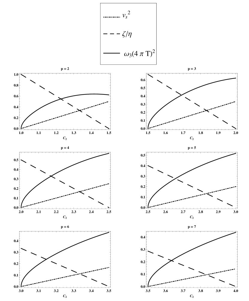
Figure 4: Plots of the dimensionless quantities: the speed of sound, ratio of bulk to shear viscosities, and $w_{3}(4\pi T)^{2}$, as a function of the free parameter $c_{2}$ appearing in the metric. Each plot corresponds to a different number of spatial dimensions $p$. Only a physical region where both $v_{s}^{2}$ and $\zeta$ are positive is shown. Note that all of the specified quantities vary with $c_{2}$ and $p$, and are thus not universal in the same sense as $\eta/s$.

21 Comparison with the shear mode

Though we have exclusively dealt with the sound mode in this chapter, we now compare our results to similar ones from the shear mode. Recall the shear dispersion relation (119),

$$w(q)_{\rm shear}=-iD_{\eta}q^{2}-iD_{\eta}^{2}\tau_{\rm shear}q^{4}+\mathcal{O}(q^{6})$$ (331)

where

$$D_{\eta}=\frac{\eta}{Ts}=\frac{1}{4\pi T}.$$ (332)

A formula for $\tau_{\rm shear}$ was given in the previous chapter (193) and in the paper [1]. This formula is applicable to a wide variety of metrics, including the special metrics we have considered in this chapter. Using the special metric (265)-(269), and the relationship (270) in this formula yields the result (195):

$$\tau_{\rm shear}=\frac{1}{4\pi T}H_{n}\left(2-\frac{p}{c_{2}}\right)=\frac{1}{4\pi T}H_{n}\left(\frac{2w_{1}^{2}}{1+w_{1}^{2}}\right).$$ (333)

Before the work of [90], it was thought that $\tau_{\rm shear}=\tau_{\pi}$, but as explained in section (5.3), the authors of the aforementioned paper showed that the coefficient of the $q^{4}$ term contains not only $\tau_{\pi}$, but also contributions from (currently unformulated) third order hydrodynamics. We can now determine these unknown contributions for the special class of metrics we are considering.

As in Sec. 5.3, let us parametrize

$$\tau_{\rm shear}=\tau_{\pi}+\Delta$$ (334)

where $\Delta$ denotes the unknown contributions from third order hydrodynamics. Combining (333) and (322) allows one to solve for $\Delta$. Evidently,

$$\Delta=\left(\frac{pv_{s}^{2}-1}{p\left(1-v_{s}^{2}\right)}\right)(\tau_{\pi}-\tau_{\Pi})-\frac{1+v_{s}^{2}}{8\pi Tv_{s}^{2}}.$$ (335)

The correction $\Delta$ is not universal in the sense that the first term is not present in the case of a conformal theory. In the conformal case, $\Delta$ is still not universal, because it depends on the number of dimensions of the theory (because $v_{s}$ depends on $p$). In the future, when the particular transport coefficients which comprise $\Delta$ are known, it will be interesting to see whether there is any universal relationship between these unknown coefficients, $\tau_{\pi}$, and $\tau_{\Pi}$.

We can easily check that the formula (335) reproduces the results in the well known $SAdS_{5}$ metric, which is dual to $\mathcal{N}=4$ supersymmetric Yang-Mills theory at finite temperature. In this case, $p=3$ and $v_{s}^{2}=1/3$. Immediately, we have

$$\Delta^{SADS_{5}}=-\frac{1}{2\pi T}.$$ (336)

In [89, 90], it was found that

$$\tau^{SADS_{5}}_{\rm shear} = \frac{1-\log(2)}{2\pi T}$$ (337)

$$\tau^{SADS_{5}}_{\pi} = \frac{2-\log(2)}{2\pi T}.$$ (338)

It is clear that the relaxation time computed from the shear mode and the sound mode differ by the amount predicted by the formula (335).

22 Summary

In this chapter, we first presented a set of gauge invariant equations for sound mode perturbations on a generic black brane type background. The equations (18.1) and (250) are the main results which pertain to this topic. These equations can be used to determine the speed of sound and bulk viscosity for any metric which can be generated by a set of minimally coupled scalar fields. In order to determine the dispersion relation, one must solve these equations perturbatively in $q$, applying the incoming wave boundary condition at the horizon, and Dirichlet boundary condition at $r=\infty$.

The gauge invariant equations are quite complicated, and so far a general analytic solution has eluded us, though we did present a solution for a particular class of metrics. These metrics are not necessarily conformal, and contain an arbitrary number of spatial dimensions $p$ with $p>2$. Metrics which obey (265) and (269) have speed of sound and bulk viscosity given by (289) and (290). These results are a generalization of the results of [101], and include both Dp-brane, and Schwarzschild AdS black hole metrics. In addition, we have computed the coefficient of the $q^{3}$ term in the sound mode dispersion relation (321) for such a class of metrics.

Information about second order transport coefficients was presented within the context of the Israel-Stewart theory. In general, a relationship (322) between two transport coefficients $\tau_{\pi}$ and $\tau_{\Pi}$ can be determined. In the conformal case of the Schwarzschild $AdS$ metric, the relation mentioned above allows the determination of the quantity $\tau_{\pi}$, since the coefficient of $\tau_{\Pi}$ vanishes in this case. We have verified that our results agree with those calculated from different methods.

Finally, by comparing the sound mode dispersion relation to the shear mode discussed in Chapter Hydrodynamics of Strongly Coupled Non-conformal Fluids from Gauge/Gravity Duality, we were able to determine the contribution of third order hydrodynamics to the shear mode (it was pointed out that such contributions would be present in [90]).

Chapter Conclusion and Discussion

In this thesis, we started by providing a brief review of the literature on gauge/gravity duality and its phenomenological applications to strongly coupled gauge theories. The central focus throughout has been hydrodynamic dispersion relations for perturbations of a strongly coupled plasma. In Chapter Hydrodynamics of Strongly Coupled Non-conformal Fluids from Gauge/Gravity Duality, we gave a pedagogical overview of the theory of hydrodynamics and also explained in detail the gauge/gravity duality methods for computing such hydrodynamic dispersion relations. In Chapters Hydrodynamics of Strongly Coupled Non-conformal Fluids from Gauge/Gravity Duality and Hydrodynamics of Strongly Coupled Non-conformal Fluids from Gauge/Gravity Duality, we applied these methods to a general gravitational dual which is supported by one or more scalar fields.

In Chapter Hydrodynamics of Strongly Coupled Non-conformal Fluids from Gauge/Gravity Duality, the shear mode dispersion relation was computed up to order $q^{4}$ (sub-leading hydrodynamic order). The equation for $\tau_{\rm shear}$ (193) is the main result of this chapter. This result is in agreement with the original publication [1], though in this thesis completely different methods were used to derive it. This is another instance where the results from and AdS/CFT calculation agree with a calculation which uses the black hole membrane paradigm.

In Chapter Hydrodynamics of Strongly Coupled Non-conformal Fluids from Gauge/Gravity Duality, the sound mode perturbations were analyzed in the same type of gravitational dual. First, we derived the relevant gauge invariant equations (18.1), (250) for the perturbations which must be solved in order to compute the dispersion relation. These equations are general, and can be applied to any dual metric which is supported by ($r$ dependent) scalar fields. Secondly, we solved these equations analytically for a special class of metrics, which allowed us to compute the sound mode dispersion relation up to order $q^{3}$ for such metrics (284),(285),(321). Examination of these results within the context of Israel-Stewart theory of hydrodynamics leads to formulas for the speed of sound (289), bulk viscosity (290), and a relationship between two relaxation times (322). Finally, by comparing the shear mode results of Chapter Hydrodynamics of Strongly Coupled Non-conformal Fluids from Gauge/Gravity Duality to the sound mode results of Chapter Hydrodynamics of Strongly Coupled Non-conformal Fluids from Gauge/Gravity Duality, we were able to gain information about the third order hydrodynamic contributions to the shear mode dispersion relation (335). All of these formulas agree with previously known results in the literature, but also offer new information about non-conformal theories.

As mentioned in the introduction, it is desirable to find universal relations among transport coefficients, as such relations have phenomenological implications for the quark-gluon plasma. Some main results of this thesis such as the shear/sound mode dispersion relation results (193), (289), (290), (321), (322) and the third order hydrodynamic contributions to the shear mode (335) are applicable to certain non-conformal gravity duals in an arbitrary number of dimensions. However, despite the fact that these relations are applicable to many theories, they are not universal like $\eta/s$ and the relation presented in [113]. For example, the number of spatial dimensions $p$ enters explicitly into our formulas, whereas a universal relation should not depend on this quantity.

Furthermore, we stress that the class of theories examined herein is limited; it seems likely that any generalization will explicitly contain the bulk viscosity $\zeta$. We were able to eliminate this quantity because our analytical results apply only to theories which satisfy the algebraic relationship (290) between $v_{s}$ and $\zeta$.

There are many possible extensions of the work presented in this thesis. First, the sound mode gauge invariant equations equations can be solved numerically for a specified metric and set of scalar field profiles. These equations may be useful for phenomenologically based models of the quark-gluon plasma such as those of [43, 116, 130]. One chief application of these gauge invariant equations is the determination of the bulk viscosity of the dual field theory. Other methods for determining the bulk viscosity do exist, in particular the work of [125] is popular in this regard. However, this method is currently only applicable to gravity duals supported by a single scalar field, while the methods documented in this thesis can be applied to models with multiple scalar fields. For example, consider the model of [116] which uses two scalar fields to dynamically generate a soft-wall setup. Once a finite temperature generalization of this setup is created, one could use the methods detailed in this thesis to compute the bulk viscosity of this phenomenological model.

In this thesis, we focused exclusively on the hydrodynamic approximation of the dispersion relation $w(q)$, which is an expansion in powers of $q/T\ll 1$. However, it is also possible to compute the full dispersion relation $w(q)$ numerically. This was done for a conformal theory in [100], but the analysis could be extended to the special non-conformal theories considered in this thesis. Numerical computation of the dispersion relation allows one to examine the perturbation’s group velocity, (for example, see [131, 132]). One should check that the theory obeys causality for all values of the deformation parameter $c_{2}$.

It would also be desirable to increase the generality of the gauge invariant equations by including other types of matter such as gauge fields, as this would increase their utility. It is a simple matter to add additional matter fields to the linearized Einstein equations presented in Chapter Hydrodynamics of Strongly Coupled Non-conformal Fluids from Gauge/Gravity Duality, since we left the energy-momentum tensor arbitrary at this stage and only later specified to the case of scalar fields.

Another issue which should be investigated is whether there are other special cases or regimes in which the gauge invariant equations can be solved analytically. Recently, in [133], the authors find that in the high temperature regime of a single scalar gravity dual, their numerical results for the bulk viscosity agree with a simple analytic formula to a remarkable degree of precision. This observation may be an indication that a general analytical formula for the bulk viscosity exists for single scalar gravity duals. If this is the case, one should be able to determine it from the gauge invariant equations presented in this thesis. The establishment of such a formula (which was, indeed, a primary motivation for the investigation of the work in this thesis) is still highly desirable.

In this thesis we examined the dispersion relations within the context of Israel-Stewart hydrodynamics to gain information about the transport coefficients in this theory. It would be beneficial to repeat this analysis for the formulation of second order hydrodynamics by Baier et al. [90]. We have checked that for conformal theories, the sound mode dispersion relations in both formulations of hydrodynamics are identical, but it is possible that differences may exist for non-conformal theories. At present, the formulation of second order hydrodynamics presented in [90] have not been generalized to non-conformal theories, though a first step was taken by Kanitscheider et al. [128] (see also [131]); it would be interesting to combine these results with those presented here to see if any new information emerges regarding second order transport coefficients. These are all issues on which we hope to report in the future.

Chapter General Relativity Reference

This appendix contains all information necessary to construct the linearized Einstein equations (to first order in the metric perturbation) for a general energy momentum tensor. The general relativistic notations used herein are those of Weinberg [76].

Appendix A Metric Perturbations

This appendix is devoted to the expressions for the relevant general relativistic tensors when the background metric $g_{\mu\nu}$ is perturbed

$$\hat{g}_{\mu\nu}=g_{\mu\nu}+h_{\mu\nu}.$$ (339)

Before proceeding one must examine what happens to the inverse metric

$$\hat{g}^{\mu\nu}\rightarrow g^{\mu\nu}+\delta g^{\mu\nu}.$$ (340)

What is $\delta g^{\mu\nu}$? By definition, the inverse metric is defined such that

$$\hat{g}_{\mu\nu}\hat{g}^{\mu\rho} = \delta^{\rho}_{\nu},$$ (341)

$$\left(g_{\mu\nu}+h_{\mu\nu}\right)\left(g^{\mu\rho}+\delta g^{\mu\rho}\right) = \delta^{\rho}_{\nu}.$$ (342)

Expanding to linear order in $h$, we have

$$g_{\mu\nu}g^{\mu\rho}+h_{\mu\nu}g^{\mu\rho}+g_{\mu\nu}\left(\delta g^{\mu\rho}\right) = \delta^{\rho}_{\nu},$$ (343)

$$h_{\mu\nu}g^{\mu\rho}+g_{\mu\nu}\left(\delta g^{\mu\rho}\right) = 0.$$ (344)

Contracting both sides by $g^{\sigma\nu}$ yields the relation

$$\delta g^{\sigma\rho}=-g^{\sigma\nu}g^{\mu\rho}h_{\mu\nu}\equiv-h^{\sigma\rho}.$$ (345)

Thus

$$\hat{g}^{\mu\nu}=g^{\mu\nu}-h^{\mu\nu}.$$ (346)

Appendix B Christoffel Symbols

The Christoffel connection is defined as

$$\Gamma^{\lambda}_{\mu\nu}=\frac{1}{2}g^{\lambda\sigma}\left[\partial_{\mu}g_{\sigma\nu}+\partial_{\nu}g_{\sigma\mu}-\partial_{\sigma}g_{\mu\nu}\right].$$ (347)

These can be evaluated explicitly for the black brane metric (23). The non-vanishing results are

$$\Gamma^{t}_{tr} = \frac{1}{2}\mathcal{D}_{L}[g_{tt}(r)],$$ (348)

$$\Gamma^{i}_{ir} = \frac{1}{2}\mathcal{D}_{L}[g_{xx}(r)],$$ (349)

$$\Gamma^{r}_{rr} = \frac{1}{2}\mathcal{D}_{L}[g_{rr}(r)],$$ (350)

$$\Gamma^{r}_{tt} = -\frac{1}{2}g^{rr}(r)g_{tt}^{\prime}(r),$$ (351)

$$\Gamma^{r}_{ii} = -\frac{1}{2}g^{rr}(r)g_{xx}^{\prime}(r).$$ (352)

Here $i$ denotes the spatial coordinates $x_{1}...x_{p}$, and we are using the notation $\mathcal{D}_{L}$ to denote the logarithmic derivative as defined in the text (103).

Introducing perturbations over the background, one finds the change in the Christoffel symbols:

$$\delta\Gamma^{\lambda}_{\mu\nu}=\frac{1}{2}g^{\lambda\sigma}\left[\partial_{\mu}h_{\sigma\nu}+\partial_{\nu}h_{\sigma\mu}-\partial_{\sigma}h_{\mu\nu}\right]-\frac{1}{2}h^{\lambda\sigma}\left[\partial_{\mu}g_{\sigma\nu}+\partial_{\nu}g_{\sigma\mu}-\partial_{\sigma}g_{\mu\nu}\right].$$ (353)

Appendix C Covariant derivative

The definition of the covariant derivative changes with the object on which it acts. For simplicity, we will act on a vector. Generalization to higher rank tensors is straightforward and is found in any text on general relativity (cf. [76]). As in the text, the superscript $(k)$ denotes quantities which are $k$th order in the perturbation. For the background metric:

$$\nabla^{(0)}_{\mu}\xi_{\nu}=\partial_{\mu}\xi_{\nu}-\Gamma^{\lambda}_{\mu\nu}\xi_{\lambda}.$$ (354)

Supposing now that we want to examine this quantity under perturbations we straightforwardly have

$$\delta(\nabla^{(0)}_{\mu}\xi_{\nu})=\partial_{\mu}(\delta\xi_{\nu})-(\delta\Gamma^{\lambda}_{\mu\nu})\xi_{\lambda}.-\Gamma^{\lambda}_{\mu\nu}(\delta\xi_{\lambda}).$$ (355)

One application of these formulas in the text is the evaluation of

$$\delta(\Box^{(0)}\phi)\equiv\delta\left(g^{\mu\nu}\nabla^{(0)}_{\mu}\nabla^{(0)}_{\nu}\phi\right).$$ (356)

Using the above formula with $\xi=\partial_{\nu}\phi$, one has

$$\delta\left(\Box^{(0)}\phi\right) = -h^{\mu\nu}\partial_{\mu}\partial_{\nu}\phi+g^{\mu\nu}\partial_{\mu}\partial_{\nu}(\delta\phi)+h^{\mu\nu}\Gamma_{\mu\nu}^{\lambda}\partial_{\lambda}\phi$$ (357)

$$- g^{\mu\nu}(\delta\Gamma_{\mu\nu}^{\lambda})\partial_{\lambda}\phi-g^{\mu\nu}\Gamma_{\mu\nu}^{\lambda}\partial_{\lambda}(\delta\phi).$$

Appendix D Ricci Tensor and Ricci Scalar

By definition, the background Ricci tensor is given by

$$R^{(0)}_{\mu\nu}=\partial_{\nu}\Gamma^{\lambda}_{\lambda\mu}-\partial_{\lambda}\Gamma^{\lambda}_{\mu\nu}+\Gamma^{\eta}_{\mu\lambda}\Gamma^{\lambda}_{\nu\eta}-\Gamma^{\eta}_{\mu\nu}\Gamma^{\lambda}_{\lambda\eta}.$$ (358)

It’s components can be explicitly evaluated for the ‘black brane’ type metric given in (23). The results are

$$F_{t}(r) \equiv g^{tt}R^{(0)}_{tt}=\frac{1}{2\sqrt{-g}}\partial_{r}\left(\sqrt{-g}g^{rr}\mathcal{D}_{L}[g_{tt}]\right),$$ (359)

$$F_{x}(r) \equiv g^{ii}R^{(0)}_{ii}=\frac{1}{2\sqrt{-g}}\partial_{r}\left(\sqrt{-g}g^{rr}\mathcal{D}_{L}[g_{xx}]\right),$$ (360)

$$F_{r}(r) \equiv g^{rr}R^{(0)}_{rr}=\frac{1}{4g_{tt}^{\,\prime}}\partial_{r}\left(g_{tt}g^{rr}\mathcal{D}_{L}[g_{tt}]^{2}\right)+\frac{p}{4g_{xx}^{\,\prime}}\partial_{r}\left(g_{xx}g^{rr}\mathcal{D}_{L}[g_{xx}]^{2}\right).$$ (361)

where we have defined the shorthand notation $F_{t}$, $F_{x}$ and $F_{r}$ for convenience.

Combinations which appear frequently in the text are

$$F_{t}-F_{x}=\frac{1}{2\sqrt{-g}}\partial_{r}\left(\sqrt{-g}g^{rr}\mathcal{D}_{L}[f]\right),$$ (362)

and

$$F_{t}-F_{r}=\frac{p}{2}g^{rr}\mathcal{D}_{L}[g_{xx}]\mathcal{D}_{L}\left[\frac{\sqrt{fg_{rr}}}{\mathcal{D}_{L}[g_{xx}]}\right],$$ (363)

where $f$ is defined as in the text (102).

To first order in the perturbation, the Ricci tensor is expanded as expected

$$R^{(1)}_{\mu\nu}=\partial_{\nu}\delta\Gamma^{\lambda}_{\lambda\mu}-\partial_{\lambda}\delta\Gamma^{\lambda}_{\nu\mu}+\delta\Gamma^{\eta}_{\mu\lambda}\Gamma^{\lambda}_{\nu\eta}+\Gamma^{\eta}_{\mu\lambda}\delta\Gamma^{\lambda}_{\nu\eta}-\delta\Gamma^{\eta}_{\mu\nu}\Gamma^{\lambda}_{\lambda\eta}-\Gamma^{\eta}_{\mu\nu}\delta\Gamma^{\lambda}_{\lambda\eta}.$$ (364)

The Ricci Scalar is defined as

$$R^{(0)}\equiv g^{\mu\nu}R^{(0)}_{\mu\nu},$$ (365)

and in the black brane background takes the form

$$R^{(0)}=F_{t}+pF_{x}+F_{r}.$$ (366)

To first order in the perturbation,

$$R^{(1)}=g^{\mu\nu}R^{(1)}_{\mu\nu}-h^{\mu\nu}R^{(0)}_{\mu\nu}.$$ (367)

One must take great care when raising and lowering indices here. For example, consider the quantity $R^{\mu\nu}_{(1)}$. This notation means $\delta\left(R^{\mu\nu}_{(0)}\right)$, as follows

$$R^{\mu\nu}_{(1)} = \delta\left[g^{\mu\alpha}g^{\nu\beta}R_{\alpha\beta}^{(0)}\right]$$ (368)

$$= R_{\alpha\beta}^{(1)}g^{\mu\alpha}g^{\nu\beta}-R_{\alpha\beta}^{(0)}\left[h^{\mu\alpha}g^{\nu\beta}+g^{\mu\alpha}h^{\nu\beta}\right].$$

Notice that $R^{\mu\nu}_{(1)}\neq R_{\alpha\beta}^{(1)}g^{\mu\alpha}g^{\nu\beta}$, there are extra terms that come from the perturbation metric which raises the indices.

Appendix E Einstein Equations

The background Einstein equations are

$$R^{(0)}_{\mu\nu}-\frac{1}{2}R^{(0)}g_{\mu\nu}=-8\pi G_{p+2}T^{(0)}_{\mu\nu}.$$ (369)

Here, $G_{p+2}$ denotes gravitational constant in $p+2$ dimensions, and $T^{(0)}_{\mu\nu}$ is the background energy momentum tensor containing information about what matter supports the metric. The perturbed equations are straightforwardly given as

$$R^{(1)}_{\mu\nu}-\frac{1}{2}R^{(1)}g_{\mu\nu}-\frac{1}{2}R^{(0)}h_{\mu\nu}=-8\pi G_{p+2}T^{(1)}_{\mu\nu}.$$ (370)

To arrive at the linearized Einstein equations given in the text, examine the quantity

$$G^{\mu\,(1)}_{\,\nu}=-8\pi G_{p+2}T^{\mu\,(1)}_{\,\nu},$$ (371)

which means

$$\delta\left(g^{\mu\lambda}R_{\nu\lambda}^{(0)}-\frac{1}{2}g^{\alpha\beta}R_{\alpha\beta}^{(0)}\delta^{\mu}_{\,\nu}\right) = -8\pi G_{p+2}\delta\left(g_{\nu\lambda}T^{\mu\lambda}_{(0)}\right),$$ (372)

$$g^{\mu\lambda}R^{(1)}_{\nu\lambda}-h^{\mu\lambda}R_{\nu\lambda}^{(0)}-\frac{1}{2}\delta^{\mu}_{\,\nu}\left[g^{\alpha\beta}R^{(1)}_{\alpha\beta}-h^{\alpha\beta}R_{\alpha\beta}^{(0)}\right] = -8\pi G_{p+2}\left(T^{\mu\lambda}_{(1)}g_{\nu\lambda}+T^{\mu\lambda}_{(0)}h_{\nu\lambda}\right).$$

(373)

In deriving this equation, we have used the fact that the Kronecker delta is unchanged under any perturbation. Explicit evaluation of the components of this tensor equation for the black brane metric (23) leads to the equations given in the text (95 - 97) and (6.3 - 110).

We have left the background energy momentum tensor arbitrary at this phase. It needs to be computed separately for the particular set of matter fields under consideration. This is done for scalar field theory in Chapter Hydrodynamics of Strongly Coupled Non-conformal Fluids from Gauge/Gravity Duality.

Chapter Techniques used in solving differential equations

This appendix contains some details regarding the techniques used to solve the differential equations in the text.

Appendix F Reduction of Order

The technique of reduction of order can be used to help solve second order linear differential equations. This technique is useful if one solution of a homogeneous equation is known, and one is searching for the second linearly independent solution.

Consider the homogeneous equation

$$y^{\prime\prime}(x)+p(x)y^{\prime}(x)+q(x)y(x)=0,$$ (374)

and assume that we know one solution $y_{1}(x)$ which satisfies this equation. To find a second solution, make the ansatz

$$y_{2}(x)=y_{1}(x)v(x).$$ (375)

Substituting this into the above equation results in

$$v^{\prime\prime}(x)y_{1}(x) + 2v^{\prime}(x)y_{1}^{\prime}(x)+y_{1}^{\prime\prime}(x)v(x)$$ (376)

$$+ p(x)\left[y_{1}^{\prime}(x)v(x)+y_{1}(x)v^{\prime}(x)\right]+q(x)y_{1}(x)v(x)=0.$$

or

$$v^{\prime\prime}(x)y_{1}(x) + v^{\prime}(x)\left[2y_{1}^{\prime}(x)+p(x)y_{1}(x)\right]$$ (377)

$$+ v(x)\left[y_{1}^{\prime\prime}(x)+p(x)y_{1}^{\prime}(x)+q(x)y_{1}(x)\right]=0.$$

Using the fact that $y_{1}(x)$ satisfies the differential equation, the last term vanishes, and we are left with the first order differential equation for $v^{\prime}(x)$:

$$v^{\prime\prime}(x)+v^{\prime}(x)\left[2\frac{y_{1}^{\prime}(x)}{y_{1}(x)}+p(x)\right]=0.$$ (378)

This can then be easily integrated to find $v^{\prime}(x)$

$$v^{\prime}(x) = v_{0}\exp\left\{-\int\left(2\frac{y_{1}^{\prime}(x)}{y_{1}(x)}+p(x)\right)\,dx\right\}$$ (379)

$$v^{\prime}(x) = \frac{v_{0}}{y_{1}(x)^{2}}\exp\left\{-\int p(x)\,dx\right\}$$ (380)

where $v_{0}$ is a arbitrary constant. $v(x)$ is then trivially found by performing another integration.

Appendix G Variation of parameters

One fundamental technique used in obtaining general solutions to inhomogeneous differential equations is the method of ‘Variation of Parameters’. The method can be used to find a general solution to a second order linear differential equation if the solution to the associated homogeneous equation is known.

The theory behind the method can be found in any textbook on differential equations. Here, we simply present the essential formulas. Consider a differential equation

$$y^{\prime\prime}(x)+p(x)y^{\prime}(x)+q(x)y(x)=g(x),$$ (381)

and assume that the functions $y_{1}(x)$ and $y_{2}(x)$ are linearly independent, and satisfy the associated homogeneous equation. That is,

$$y_{1}^{\prime\prime}(x)+p(x)y_{1}^{\prime}(x)+q(x)y_{1}^{\prime}(x)=0,$$ (382)

and similarly for $y_{2}(x)$. It can be shown that the function $y_{p}(x)$ is a solution to the inhomogeneous equation, where

$$y_{p}(x)=y_{2}(x)\int\frac{y_{1}(x)g(x)}{W(x)}\,dx-y_{1}(x)\int\frac{y_{2}(x)g(x)}{W(x)}.$$ (383)

Here, $W(x)$ is the Wronskian

$$W(x)\equiv y_{1}(x)y_{2}^{\prime}(x)-y_{1}^{\prime}(x)y_{2}(x).$$ (384)

To arrive at the form of the function $y_{p}$ used in the text (302), let us define

$$h(x)\equiv\frac{y_{2}(x)}{y_{1}(x)}.$$ (385)

Then,

$$W(x)=h^{\prime}(x)y_{1}^{2}(x),$$ (386)

and

$$y_{p}(x)=y_{1}(x)\left[h(x)\int\frac{g(x)}{y_{1}(x)h^{\prime}(x)}\,dx-\int\frac{h(x)g(x)}{h^{\prime}(x)y_{1}(x)}\right].$$ (387)

One can see that this is equivalent to

$$y_{p}(x)=y_{1}(x)\int h^{\prime}(x)\int^{x}\frac{g(z)}{y_{1}(z)h^{\prime}(z)}\,dz\,dx$$ (388)

by performing an integration by parts.

References

- [1] J. I. Kapusta and T. Springer, “Shear Transport Coefficients from Gauge/Gravity Correspondence,” Phys. Rev. D78 (2008) 066017, arXiv:0806.4175 [hep-th].
- [2] T. Springer, “Sound Mode Hydrodynamics from Bulk Scalar Fields,” Phys. Rev. D79 (2009) 046003, arXiv:0810.4354 [hep-th].
- [3] T. Springer, “Second order hydrodynamics for a special class of gravity duals,” Phys. Rev. D79 (2009) 086003, arXiv:0902.2566 [hep-th].
- [4] STAR Collaboration, J. Adams et al., “Experimental and theoretical challenges in the search for the quark gluon plasma: The STAR collaboration’s critical assessment of the evidence from RHIC collisions,” Nucl. Phys. A757 (2005) 102–183, arXiv:nucl-ex/0501009.
- [5] PHENIX Collaboration, K. Adcox et al., “Formation of dense partonic matter in relativistic nucleus nucleus collisions at RHIC: Experimental evaluation by the PHENIX collaboration,” Nucl. Phys. A757 (2005) 184–283, arXiv:nucl-ex/0410003.
- [6] BRAHMS Collaboration, I. Arsene et al., “Quark Gluon Plasma an Color Glass Condensate at RHIC? The perspective from the BRAHMS experiment,” Nucl. Phys. A757 (2005) 1–27, arXiv:nucl-ex/0410020.
- [7] B. B. Back et al., “The PHOBOS perspective on discoveries at RHIC,” Nucl. Phys. A757 (2005) 28–101, arXiv:nucl-ex/0410022.
- [8] J. M. Maldacena, “The large N limit of superconformal field theories and supergravity,” Adv. Theor. Math. Phys. 2 (1998) 231–252, arXiv:hep-th/9711200.
- [9] E. Witten, “Anti-de Sitter space and holography,” Adv. Theor. Math. Phys. 2 (1998) 253–291, arXiv:hep-th/9802150.
- [10] S. S. Gubser, I. R. Klebanov, and A. M. Polyakov, “Gauge theory correlators from non-critical string theory,” Phys. Lett. B428 (1998) 105–114, arXiv:hep-th/9802109.
- [11] L. McLerran, “The Color Glass Condensate and Glasma,” arXiv:0804.1736 [hep-ph].
- [12] H. Weigert, “Evolution at small x(bj): The color glass condensate,” Prog. Part. Nucl. Phys. 55 (2005) 461–565, arXiv:hep-ph/0501087.
- [13] E. Shuryak, “Physics of Strongly coupled Quark-Gluon Plasma,” Prog. Part. Nucl. Phys. 62 (2009) 48–101, arXiv:0807.3033 [hep-ph].
- [14] D. Banerjee, J. K. Nayak, and R. Venugopalan, “Two introductory lectures on high energy QCD and heavy ion collisions,” arXiv:0810.3553 [hep-ph].
- [15] O. Aharony, S. S. Gubser, J. M. Maldacena, H. Ooguri, and Y. Oz, “Large N field theories, string theory and gravity,” Phys. Rept. 323 (2000) 183–386, arXiv:hep-th/9905111.
- [16] S. S. Gubser and A. Karch, “From gauge-string duality to strong interactions: a Pedestrian’s Guide,” arXiv:0901.0935 [hep-th].
- [17] R. C. Myers and S. E. Vazquez, “Quark Soup al dente: Applied Superstring Theory,” Class. Quant. Grav. 25 (2008) 114008, arXiv:0804.2423 [hep-th].
- [18] J. D. Edelstein, J. P. Shock, and D. Zoakos, “The AdS/CFT Correspondence and Non-perturbative QCD,” arXiv:0901.2534 [hep-ph].
- [19] I. R. Klebanov, “QCD and string theory,” Int. J. Mod. Phys. A21 (2006) 1831–1843, arXiv:hep-ph/0509087.
- [20] E. Witten, “Bound states of strings and p-branes,” Nucl. Phys. B460 (1996) 335–350, arXiv:hep-th/9510135.
- [21] G. T. Horowitz and A. Strominger, “Black strings and P-branes,” Nucl. Phys. B360 (1991) 197–209.
- [22] J. Polchinski, String theory. Volume I: An introduction to the bosonic string. Volume II: Superstring theory and beyond. Cambridge University Press, Cambridge (UK), 1998.
- [23] J. X. Lu, “ADM masses for black strings and p-branes,” Phys. Lett. B313 (1993) 29–34, arXiv:hep-th/9304159.
- [24] A. W. Peet, “TASI lectures on black holes in string theory,” arXiv:hep-th/0008241.
- [25] O. Aharony, A. Fayyazuddin, and J. M. Maldacena, “The large N limit of N = 2,1 field theories from three- branes in F-theory,” JHEP 07 (1998) 013, arXiv:hep-th/9806159.
- [26] A. Karch and E. Katz, “Adding flavor to AdS/CFT,” JHEP 06 (2002) 043, arXiv:hep-th/0205236.
- [27] E. Witten, “Anti-de Sitter space, thermal phase transition, and confinement in gauge theories,” Adv. Theor. Math. Phys. 2 (1998) 505–532, arXiv:hep-th/9803131.
- [28] J. Polchinski and M. J. Strassler, “The string dual of a confining four-dimensional gauge theory,” arXiv:hep-th/0003136.
- [29] J. M. Maldacena and C. Nunez, “Towards the large N limit of pure N = 1 super Yang Mills,” Phys. Rev. Lett. 86 (2001) 588–591, arXiv:hep-th/0008001.
- [30] I. R. Klebanov and M. J. Strassler, “Supergravity and a confining gauge theory: Duality cascades and chiSB-resolution of naked singularities,” JHEP 08 (2000) 052, arXiv:hep-th/0007191.
- [31] M. Kruczenski, D. Mateos, R. C. Myers, and D. J. Winters, “Towards a holographic dual of large-N(c) QCD,” JHEP 05 (2004) 041, arXiv:hep-th/0311270.
- [32] T. Sakai and S. Sugimoto, “Low energy hadron physics in holographic QCD,” Prog. Theor. Phys. 113 (2005) 843–882, arXiv:hep-th/0412141.
- [33] J. Polchinski and M. J. Strassler, “Hard scattering and gauge/string duality,” Phys. Rev. Lett. 88 (2002) 031601, arXiv:hep-th/0109174.
- [34] J. Erlich, E. Katz, D. T. Son, and M. A. Stephanov, “QCD and a Holographic Model of Hadrons,” Phys. Rev. Lett. 95 (2005) 261602, arXiv:hep-ph/0501128.
- [35] A. Karch, E. Katz, D. T. Son, and M. A. Stephanov, “Linear Confinement and AdS/QCD,” Phys. Rev. D74 (2006) 015005, arXiv:hep-ph/0602229.
- [36] S. S. Gubser and A. Nellore, “Mimicking the QCD equation of state with a dual black hole,” Phys. Rev. D78 (2008) 086007, arXiv:0804.0434 [hep-th].
- [37] S. S. Gubser, A. Nellore, S. S. Pufu, and F. D. Rocha, “Thermodynamics and bulk viscosity of approximate black hole duals to finite temperature quantum chromodynamics,” Phys. Rev. Lett. 101 (2008) 131601, arXiv:0804.1950 [hep-th].
- [38] O. Andreev, “Some Thermodynamic Aspects of Pure Glue, Fuzzy Bags and Gauge/String Duality,” Phys. Rev. D76 (2007) 087702, arXiv:0706.3120 [hep-ph].
- [39] K. Kajantie, T. Tahkokallio, and J.-T. Yee, “Thermodynamics of AdS/QCD,” JHEP 01 (2007) 019, arXiv:hep-ph/0609254.
- [40] U. Gursoy and E. Kiritsis, “Exploring improved holographic theories for QCD: Part I,” JHEP 02 (2008) 032, arXiv:0707.1324 [hep-th].
- [41] U. Gursoy, E. Kiritsis, and F. Nitti, “Exploring improved holographic theories for QCD: Part II,” JHEP 02 (2008) 019, arXiv:0707.1349 [hep-th].
- [42] U. Gursoy, E. Kiritsis, L. Mazzanti, and F. Nitti, “Deconfinement and Gluon Plasma Dynamics in Improved Holographic QCD,” Phys. Rev. Lett. 101 (2008) 181601, arXiv:0804.0899 [hep-th].
- [43] U. Gursoy, E. Kiritsis, L. Mazzanti, and F. Nitti, “Holography and Thermodynamics of 5D Dilaton-gravity,” arXiv:0812.0792 [hep-th].
- [44] U. Gursoy, E. Kiritsis, G. Michalogiorgakis, and F. Nitti, “Thermal Transport and Drag Force in Improved Holographic QCD,” arXiv:0906.1890 [hep-ph].
- [45] N. Iqbal and H. Liu, “Universality of the hydrodynamic limit in AdS/CFT and the membrane paradigm,” arXiv:0809.3808 [hep-th].
- [46] A. Buchel and J. T. Liu, “Universality of the shear viscosity in supergravity,” Phys. Rev. Lett. 93 (2004) 090602, arXiv:hep-th/0311175.
- [47] P. Kovtun, D. T. Son, and A. O. Starinets, “Holography and hydrodynamics: Diffusion on stretched horizons,” JHEP 10 (2003) 064, arXiv:hep-th/0309213.
- [48] P. Romatschke and U. Romatschke, “Viscosity Information from Relativistic Nuclear Collisions: How Perfect is the Fluid Observed at RHIC?,” Phys. Rev. Lett. 99 (2007) 172301, arXiv:0706.1522 [nucl-th].
- [49] H. Song and U. W. Heinz, “Suppression of elliptic flow in a minimally viscous quark- gluon plasma,” Phys. Lett. B658 (2008) 279–283, arXiv:0709.0742 [nucl-th].
- [50] P. Romatschke, “Fluid turbulence and eddy viscosity in relativistic heavy- ion collisions,” Prog. Theor. Phys. Suppl. 174 (2008) 137–144, arXiv:0710.0016 [nucl-th].
- [51] H. Song and U. W. Heinz, “Causal viscous hydrodynamics in 2+1 dimensions for relativistic heavy-ion collisions,” Phys. Rev. C77 (2008) 064901, arXiv:0712.3715 [nucl-th].
- [52] J. D. Bekenstein, “Black holes and entropy,” Phys. Rev. D7 (1973) 2333–2346.
- [53] J. D. Bekenstein, “Generalized second law of thermodynamics in black hole physics,” Phys. Rev. D9 (1974) 3292–3300.
- [54] S. W. Hawking, “Particle Creation by Black Holes,” Commun. Math. Phys. 43 (1975) 199–220.
- [55] A. Zee, Quantum field theory in a nutshell. Princeton University Pressa: Princeton, NJ, 2003.
- [56] C. P. Herzog, “A holographic prediction of the deconfinement temperature,” Phys. Rev. Lett. 98 (2007) 091601, arXiv:hep-th/0608151.
- [57] C. A. Ballon Bayona, H. Boschi-Filho, N. R. F. Braga, and L. A. Pando Zayas, “On a holographic model for confinement / deconfinement,” Phys. Rev. D77 (2008) 046002, arXiv:0705.1529 [hep-th].
- [58] J. Erdmenger, N. Evans, I. Kirsch, and E. Threlfall, “Mesons in Gauge/Gravity Duals - A Review,” Eur. Phys. J. A35 (2008) 81–133, arXiv:0711.4467 [hep-th].
- [59] L. Da Rold and A. Pomarol, “Chiral symmetry breaking from five dimensional spaces,” Nucl. Phys. B721 (2005) 79–97, arXiv:hep-ph/0501218.
- [60] L. Da Rold and A. Pomarol, “The scalar and pseudoscalar sector in a five-dimensional approach to chiral symmetry breaking,” JHEP 01 (2006) 157, arXiv:hep-ph/0510268.
- [61] G. F. de Teramond and S. J. Brodsky, “The hadronic spectrum of a holographic dual of QCD,” Phys. Rev. Lett. 94 (2005) 201601, arXiv:hep-th/0501022.
- [62] T. Gherghetta, J. I. Kapusta, and T. M. Kelley, “Chiral Symmetry Breaking in Soft-Wall AdS/QCD,” arXiv:0902.1998 [hep-ph].
- [63] D. Mateos, R. C. Myers, and R. M. Thomson, “Holographic phase transitions with fundamental matter,” Phys. Rev. Lett. 97 (2006) 091601, arXiv:hep-th/0605046.
- [64] C. Hoyos-Badajoz, K. Landsteiner, and S. Montero, “Holographic Meson Melting,” JHEP 04 (2007) 031, arXiv:hep-th/0612169.
- [65] J. Babington, J. Erdmenger, N. J. Evans, Z. Guralnik, and I. Kirsch, “Chiral symmetry breaking and pions in non-supersymmetric gauge / gravity duals,” Phys. Rev. D69 (2004) 066007, arXiv:hep-th/0306018.
- [66] I. Kirsch, “Generalizations of the AdS/CFT correspondence,” Fortsch. Phys. 52 (2004) 727–826, arXiv:hep-th/0406274.
- [67] C. P. Herzog, A. Karch, P. Kovtun, C. Kozcaz, and L. G. Yaffe, “Energy loss of a heavy quark moving through N = 4 supersymmetric Yang-Mills plasma,” JHEP 07 (2006) 013, arXiv:hep-th/0605158.
- [68] S. S. Gubser, “Drag force in AdS/CFT,” Phys. Rev. D74 (2006) 126005, arXiv:hep-th/0605182.
- [69] H. Liu, K. Rajagopal, and U. A. Wiedemann, “Calculating the jet quenching parameter from AdS/CFT,” Phys. Rev. Lett. 97 (2006) 182301, arXiv:hep-ph/0605178.
- [70] R. A. Janik and R. B. Peschanski, “Asymptotic perfect fluid dynamics as a consequence of AdS/CFT,” Phys. Rev. D73 (2006) 045013, arXiv:hep-th/0512162.
- [71] R. A. Janik and R. B. Peschanski, “Gauge / gravity duality and thermalization of a boost- invariant perfect fluid,” Phys. Rev. D74 (2006) 046007, arXiv:hep-th/0606149.
- [72] J. J. Friess, S. S. Gubser, G. Michalogiorgakis, and S. S. Pufu, “Expanding plasmas and quasinormal modes of anti-de Sitter black holes,” JHEP 04 (2007) 080, arXiv:hep-th/0611005.
- [73] Y. V. Kovchegov and A. Taliotis, “Early time dynamics in heavy ion collisions from AdS/CFT correspondence,” Phys. Rev. C76 (2007) 014905, arXiv:0705.1234 [hep-ph].
- [74] P. M. Chesler and L. G. Yaffe, “Horizon formation and far-from-equilibrium isotropization in supersymmetric Yang-Mills plasma,” arXiv:0812.2053 [hep-th].
- [75] Landau, L.D. and Lifshitz, E.M, Fluid Mechanics. 2nd edition, Pergamon Press, New York, 1987.
- [76] Weinberg, S., Gravitation and Cosmology: Principles and Applications of the General Theory of Relativity. Wiley & Sons: New York, July, 1972.
- [77] Kapusta, J.I. and Gale, C., Finite-Temperature Field Theory: Principles and Applications. 2nd edition, Cambridge Monographs on Mathematical Physics. Cambridge University Press, Cambridge, 2006.
- [78] D. T. Son and A. O. Starinets, “Viscosity, Black Holes, and Quantum Field Theory,” Ann. Rev. Nucl. Part. Sci. 57 (2007) 95–118, arXiv:0704.0240 [hep-th].
- [79] P. Kovtun and L. G. Yaffe, “Hydrodynamic fluctuations, long-time tails, and supersymmetry,” Phys. Rev. D68 (2003) 025007, arXiv:hep-th/0303010.
- [80] I. Müller, “Zum Paradoxon der Wärmeleitungstheorie,” Zeitschrift fur Physik 198 (1967) 329–344.
- [81] W. Israel, “Nonstationary irreversible thermodynamics: A Causal relativistic theory,” Ann. Phys. 100 (1976) 310–331.
- [82] W. Israel and J. M. Stewart, “Transient relativistic thermodynamics and kinetic theory,” Ann. Phys. 118 (1979) 341–372.
- [83] W. A. Hiscock and L. Lindblom, “Stability and causality in dissipative relativistic fluids,” Annals Phys. 151 (1983) 466–496.
- [84] R. P. Geroch, “Relativistic theories of dissipative fluids,” J. Math. Phys. 36 (1995) 4226.
- [85] R. P. Geroch, “On Hyperbolic ”Theories” of Relativistic Dissipative Fluids,” arXiv:gr-qc/0103112.
- [86] P. Kostadt and M. Liu, “Causality and stability of the relativistic diffusion equation,” Phys. Rev. D62 (2000) 023003.
- [87] P. Kostadt and M. Liu, “Alleged acausality of the diffusion equations: A reply,” Phys. Rev. D64 (2001) 088504.
- [88] W. A. Hiscock and L. Lindblom, “Generic instabilities in first-order dissipative relativistic fluid theories,” Phys. Rev. D31 (1985) 725–733.
- [89] M. Natsuume and T. Okamura, “Causal hydrodynamics of gauge theory plasmas from AdS/CFT duality,” Phys. Rev. D77 (erratum: D78) (2008) 066014 (erratum: 089902), arXiv:0712.2916 [hep-th].
- [90] R. Baier, P. Romatschke, D. T. Son, A. O. Starinets, and M. A. Stephanov, “Relativistic viscous hydrodynamics, conformal invariance, and holography,” JHEP 04 (2008) 100, arXiv:0712.2451 [hep-th].
- [91] D. Molnar and M. Gyulassy, “Saturation of elliptic flow at RHIC: Results from the covariant elastic parton cascade model MPC,” Nucl. Phys. A697, (erratum: A703) (2002) 495–520, (erratum: 893–894), arXiv:nucl-th/0104073.
- [92] P. Huovinen, P. F. Kolb, U. W. Heinz, P. V. Ruuskanen, and S. A. Voloshin, “Radial and elliptic flow at RHIC: further predictions,” Phys. Lett. B503 (2001) 58–64, arXiv:hep-ph/0101136.
- [93] P. Huovinen, “Hydrodynamical description of collective flow,” arXiv:nucl-th/0305064.
- [94] G. Policastro, D. T. Son, and A. O. Starinets, “The shear viscosity of strongly coupled N = 4 supersymmetric Yang-Mills plasma,” Phys. Rev. Lett. 87 (2001) 081601, arXiv:hep-th/0104066.
- [95] D. T. Son and A. O. Starinets, “Minkowski-space correlators in AdS/CFT correspondence: Recipe and applications,” JHEP 09 (2002) 042, arXiv:hep-th/0205051.
- [96] G. Policastro, D. T. Son, and A. O. Starinets, “From AdS/CFT correspondence to hydrodynamics,” JHEP 09 (2002) 043, arXiv:hep-th/0205052.
- [97] G. Policastro, D. T. Son, and A. O. Starinets, “From AdS/CFT correspondence to hydrodynamics. II: Sound waves,” JHEP 12 (2002) 054, arXiv:hep-th/0210220.
- [98] C. P. Herzog, “The hydrodynamics of M-theory,” JHEP 12 (2002) 026, arXiv:hep-th/0210126.
- [99] C. P. Herzog, “The sound of M-theory,” Phys. Rev. D68 (2003) 024013, arXiv:hep-th/0302086.
- [100] P. K. Kovtun and A. O. Starinets, “Quasinormal modes and holography,” Phys. Rev. D72 (2005) 086009, arXiv:hep-th/0506184.
- [101] J. Mas and J. Tarrio, “Hydrodynamics from the Dp-brane,” JHEP 05 (2007) 036, arXiv:hep-th/0703093.
- [102] K. Thorne, R. Price, and D. MacDonald, Black holes: The membrane paradigm. Yale University Press: New Haven, CT, 1986.
- [103] O. Saremi, “Shear waves, sound waves on a shimmering horizon,” arXiv:hep-th/0703170.
- [104] M. Fujita, “Non-equilibrium thermodynamics near the horizon and holography,” JHEP 10 (2008) 031, arXiv:0712.2289 [hep-th].
- [105] M. Natsuume, “Causal hydrodynamics and the membrane paradigm,” Phys. Rev. D78 (2008) 066010, arXiv:0807.1392 [hep-th].
- [106] S. Bhattacharyya, V. E. Hubeny, S. Minwalla, and M. Rangamani, “Nonlinear Fluid Dynamics from Gravity,” JHEP 02 (2008) 045, arXiv:0712.2456 [hep-th].
- [107] M. Van Raamsdonk, “Black Hole Dynamics From Atmospheric Science,” JHEP 05 (2008) 106, arXiv:0802.3224 [hep-th].
- [108] M. Haack and A. Yarom, “Nonlinear viscous hydrodynamics in various dimensions using AdS/CFT,” JHEP 10 (2008) 063, arXiv:0806.4602 [hep-th].
- [109] S. Bhattacharyya, R. Loganayagam, I. Mandal, S. Minwalla, and A. Sharma, “Conformal Nonlinear Fluid Dynamics from Gravity in Arbitrary Dimensions,” JHEP 12 (2008) 116, arXiv:0809.4272 [hep-th].
- [110] J. Erdmenger, M. Haack, M. Kaminski, and A. Yarom, “Fluid dynamics of R-charged black holes,” JHEP 01 (2009) 055, arXiv:0809.2488 [hep-th].
- [111] N. Banerjee et al., “Hydrodynamics from charged black branes,” arXiv:0809.2596 [hep-th].
- [112] S. Bhattacharyya et al., “Forced Fluid Dynamics from Gravity,” JHEP 02 (2009) 018, arXiv:0806.0006 [hep-th].
- [113] M. Haack and A. Yarom, “Universality of second order transport coefficients from the gauge-string duality,” Nucl. Phys. B813 (2009) 140–155, arXiv:0811.1794 [hep-th].
- [114] Mukhanov, V., Physical Foundations of Cosmology. Cambridge University Press, Cambridge, 2005.
- [115] A. O. Starinets, “Quasinormal spectrum and the black hole membrane paradigm,” Phys. Lett. B670 (2009) 442–445, arXiv:0806.3797 [hep-th].
- [116] B. Batell and T. Gherghetta, “Dynamical Soft-Wall AdS/QCD,” Phys. Rev. D78 (2008) 026002, arXiv:0801.4383 [hep-ph].
- [117] S. Carroll, Spacetime and geometry. An introduction to general relativity. Addison Wesley: San Francisco, CA, 2004.
- [118] J. Mas, “Shear viscosity from R-charged AdS black holes,” JHEP 03 (2006) 016, arXiv:hep-th/0601144.
- [119] D. T. Son and A. O. Starinets, “Hydrodynamics of R-charged black holes,” JHEP 03 (2006) 052, arXiv:hep-th/0601157.
- [120] O. Saremi, “The viscosity bound conjecture and hydrodynamics of M2- brane theory at finite chemical potential,” JHEP 10 (2006) 083, arXiv:hep-th/0601159.
- [121] K. Maeda, M. Natsuume, and T. Okamura, “Viscosity of gauge theory plasma with a chemical potential from AdS/CFT,” Phys. Rev. D73 (2006) 066013, arXiv:hep-th/0602010.
- [122] Y.-h. Gao, W.-s. Xu, and D.-f. Zeng, “Viscosity and jet quenching from holographic model,” arXiv:0707.0817 [hep-ph].
- [123] D. Kharzeev and K. Tuchin, “Bulk viscosity of QCD matter near the critical temperature,” JHEP 09 (2008) 093, arXiv:0705.4280 [hep-ph].
- [124] F. Karsch, D. Kharzeev, and K. Tuchin, “Universal properties of bulk viscosity near the QCD phase transition,” Phys. Lett. B663 (2008) 217–221, arXiv:0711.0914 [hep-ph].
- [125] S. S. Gubser, S. S. Pufu, and F. D. Rocha, “Bulk viscosity of strongly coupled plasmas with holographic duals,” JHEP 08 (2008) 085, arXiv:0806.0407 [hep-th].
- [126] H. A. Chamblin and H. S. Reall, “Dynamic dilatonic domain walls,” Nucl. Phys. B562 (1999) 133–157, arXiv:hep-th/9903225.
- [127] A. Buchel, “Bulk viscosity of gauge theory plasma at strong coupling,” Phys. Lett. B663 (2008) 286–289, arXiv:0708.3459 [hep-th].
- [128] I. Kanitscheider and K. Skenderis, “Universal hydrodynamics of non-conformal branes,” arXiv:0901.1487 [hep-th].
- [129] J. R. David, M. Mahato, and S. R. Wadia, “Hydrodynamics from the D1-brane,” arXiv:0901.2013 [hep-th].
- [130] W. de Paula, T. Frederico, H. Forkel, and M. Beyer, “Dynamical AdS/QCD with area-law confinement and linear Regge trajectories,” arXiv:0806.3830 [hep-ph].
- [131] P. Romatschke, “New Developments in Relativistic Viscous Hydrodynamics,” arXiv:0902.3663 [hep-ph].
- [132] S. Hod, “From Thermodynamics to the Bound on Viscosity,” Nucl. Phys. B819 (2009) 177–182, arXiv:0907.1144 [hep-th].
- [133] A. Cherman and A. Nellore, “Universal relations of transport coefficients from holography,” arXiv:0905.2969 [hep-th].
Chapter \thechapter General Relativity Reference