Josephson Effect in Superconductors and Superfluids

Chapter 1 Macroscopic phase coherence and Josephson effect

In this Chapter we consider systems, that at first glance may seem very different: (i) superconductors, which at temperatures larger than the critical temperature $T_{c}$ ($T_{c}$ in conventional superconductors is of order of a few $K$) turn metallic and are described by the Fermi Liquid theory, (ii) superfluid liquid He: bosonic ⁴He, $T_{c}=2.17K$ and fermionic ³He, $T_{c}=0.0025K$; and (iii) Bose-Einstein condensates of cold alkali atoms (with $T_{c}$ of the order of nano Kelvin). All these systems have one important property in common - at low temperatures they possess macroscopic coherence.

In previous Chapters it was discussed that a superconducting state is a state with a broken $U(1)$–symmetry and is thus characterized by a complex order parameter

$$\Psi=\Psi({\bf r})=|\Psi({\bf r})|e^{i\phi({\bf r})}$$ (1.1)

which represents a macroscopic wave function of a superconductor. The presence of the order parameter means that at any given moment the phase difference of $\Psi$-functions between any two macroscopically separated points in the superconductor is fixed, so that the whole sample acquires macroscopic phase coherence, or in other words, long-range order develops. One can describe a condensate of cold bosons or a superfluid He system in a similar way, since these systems are also phase coherent.

Phase coherence leads to a number of specific quantum effects. For example, in superconductors it causes the quantization of magnetic flux first considered by London. One of the most celebrated manifestations of the phase coherence property is however the Josephson effect which is the subject of the current Chapter.

Chapter 2 Josephson Effect in superconductors

In 1962 Brian Josephson predicted a curious effect occurring in a system of two weakly-linked superconductors [1]. He demonstrated that a direct current can flow between two superconductors coupled via an insulating thin layer although no external voltage is applied. Furthermore, he showed that an external voltage would give rise to a rapidly oscillating current. Josephson’s theory of a current induced between two superconductors was rather fast confirmed experimentally [2].

The Josephson effect can be understood by the following simple considerations. First of all it is important to observe that a gradient of the phase gives rise to a current

$$j=\frac{N_{s}e\hbar}{2m}\nabla\phi,$$ (2.1)

where $N_{s}$ is the number of superconducting electrons. Imagine now that instead of a uniform superconductor we deal with a superconductor with impurities: point-like, randomly distributed non-magnetic impurities. As we know, for an s-wave superconductor impurities do not affect the critical temperature, they do not destroy phase coherence in a superconductor (in accordance with Anderson’s theorem [3]). As a consequence supercurrents (2.1) can flow through the system without a problem. This situation does not change if instead of impurities distributed in the bulk we have impurities distributed solely in a plane inside a superconductor (Fig.2.1(a)).

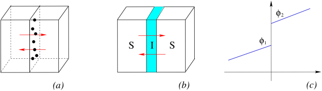
Figure 2.1: Superconductor with an “impurity plane” inside (a). Supercurrent will persist even if the plane is replaced by a thin insulating layer (b). The phase jump at the barrier separating two superconductors (c).

Supercurrents proportional to the the fixed phase gradient can flow through the plane, even though the mean spacing between the impurities is smaller than the coherence length of a superconductor. This intuitively clear picture can be generalized to the case of a somewhat more complicated system: two superconductors separated by a thin insulating layer. This nontrivial generalization was realized by Josephson and led him to the prediction of two effects named after him: a.c. and d.c. Josephson effects.

These Josephson effects are pure quantum phenomena, because electrons travel from one superconductor to the other by means of quantum mechanical tunneling through the barrier separating the two superconducting systems. The presence of a barrier, or inhomogeneity leads to the fact that the phase has a jump at the barrier (Fig. 2.1(c)). The supercurrent through the barrier is then driven by the phase difference $\phi=\phi_{2}-\phi_{1}$. Thus, a supercurrent can flow between two superconductors provided they are separated by a sufficiently thin insulating layer. This effect is referred to as first or stationary, or d.c. Josephson effect. In this case the potential difference through the barrier is equal to zero. Note, that while the superconducting coherence length is of the order of $\xi\sim 10^{4}$ Å, the thickness of the insulting layer should be of the order of $10-20$ Å, i.e. thousands of times smaller than $\xi$.

When a finite voltage bias $V$ is applied to an SIS junction, the second, non-stationary or a.c. Josephson effect can be observed. In this case the current will be oscillating between the two superconductors with a frequency $\omega$ proportional to the applied bias

$$\hbar\omega=2eV.$$ (2.2)

Since in a superconductor electrons are bound into Cooper pairs, these pairs participate in the tunneling across a barrier between two superconductors. The energy $2eV$ is then just the difference in the energy of a Cooper pair in passing from one superconductor to the other.

One can estimate a Josephson current from simple electrodynamic considerations [4]. First of all we observe, that the appearance of a current in the system is related to the excess energy $\Delta E=E(\phi)-E(\phi=0)$ associated with the junction between the two superconductors. It is clear that $\Delta E$ should be proportional to the product of two superconducting gaps $\Delta_{1}\Delta_{2}$, because if one of superconductors is absent, the excess energy vanishes. Apart from that the excess energy should be real, one can therefore conjecture its simplest possible form as follows

$$\Delta E=\alpha\int dxdy\left(|\Delta_{1}\Delta_{2}|-\frac{1}{2}(\Delta_{1}\Delta_{2}^{*}+c.c.)\right)=2\alpha\int dxdy|\Delta_{1}\Delta_{2}|(1-\cos\phi),$$ (2.3)

where $\alpha$ is a phenomenological constant describing the coupling between the two superconductors in the $x-y$ junction plane.

One can derive now from the gauge invariance principle that the supercurrent is proportional to $(\sin\phi)$. The gauge invariance requires the replacement

$$\nabla\phi\rightarrow\nabla\phi-\frac{2e}{\hbar c}{\bf A},$$ (2.4)

where ${\bf A}$ is the vector potential. For simplicity we can chose the vector potential perpendicular to the $x-y$ plane, so that integration along that axes of the r.h.s. of (2.4) gives

$$\phi_{1}-\phi_{2}-\frac{2e}{\hbar c}\int_{L}^{R}dzA_{z},$$ (2.5)

where $\phi_{1}$ is the phase of the “left” superconductor, and $\phi_{2}$ is the phase of the “right” superconductor. The excess energy becomes

$$\Delta E=2\alpha\int dx\,dy|\Delta_{1}\Delta_{2}|\left[1-\cos\left(\phi_{1}-\phi_{2}-\frac{2e}{\hbar c}\int_{L}^{R}dzA_{z}\right)\right].$$ (2.6)

Variation of this energy with respect to the potential gives

$$\delta(\Delta E)=-\frac{2e}{\hbar c}\alpha\int dx\,dy\,dz\,|\Delta_{1}\Delta_{2}|\sin\left(\phi_{1}-\phi_{2}-\frac{2e}{\hbar c}\int_{L}^{R}dzA_{z}\right)\Big{]}\delta A_{z}.$$ (2.7)

From electrodynamics we know that

$$\delta E=-\frac{1}{c}\int{\bf j}\;\delta{\bf A}\;dV,$$ (2.8)

and we get for the supercurrent

$$j=\frac{2e}{\hbar}\alpha|\Delta_{1}\Delta_{2}|\sin\left(\phi_{1}-\phi_{2}-\frac{2e}{\hbar c}\int_{L}^{R}dzA_{z}\right).$$ (2.9)

For zero vector potential we obtain the famous expression for the Josephson current

$$j=j_{c}\sin(\phi_{1}-\phi_{2}).$$ (2.10)

The current vanishes for $\phi_{1}-\phi_{2}=0$. The so-called critical current $j_{c}$ should be calculated microscopically (see Section 3).

The basic result (2.10) can be obtained in a different way. The following derivation in terms of a two-level system is due to Feynman [5]. As we discussed already, each superconductor can be considered as a macroscopic quantum state described by a wave-function $\Psi_{1,2}$ (1.1). Since the coupling between the superconductors is very weak, the state vector describing the coupled system can be written in a simple form

$$|\Psi\rangle=\Psi_{1}|1\rangle+\Psi_{2}|2\rangle.$$ (2.11)

The density of superconducting electrons in the left (right) superconductor, described by the state $|1\rangle$ ($|2\rangle$) is defined as

$$n_{i}=|\Psi_{i}|^{2}=\langle i|\Psi\rangle\langle\Psi|i\rangle,$$ (2.12)

$i=1,2$. The Schrödinger equation of motion for the state vector (2.11) reads

$$i\hbar\partial_{t}|\Psi\rangle=H|\Psi\rangle,$$ (2.13)

with the Hamiltonian

$$H=H_{1}+H_{2}+H_{int}.$$ (2.14)

Here $H_{i}=E_{i}|i\rangle\langle i|$, ($i=1,2$) and the coupling between the superconductors can be written in analogy with (2.3)

$$H_{int}=-\frac{\alpha}{2}(|1\rangle\langle 2|+|2\rangle\langle 1|).$$ (2.15)

Projection of the Eq. (2.13) on the two states gives the equations of motion for two weakly coupled superconductors

$$i\hbar\partial_{t}\Psi_{1}=E_{1}\Psi_{1}-\frac{\alpha}{2}\Psi_{2},$$

$$i\hbar\partial_{t}\Psi_{2}=E_{2}\Psi_{2}-\frac{\alpha}{2}\Psi_{1}.$$ (2.16)

Remembering that $\Psi_{i}$ can be expressed in terms of superconducting densities (see (2.12))

$$\Psi_{i}=\sqrt{n_{i}}e^{i\phi_{i}},$$ (2.17)

we can derive the final equations in terms of the densities and phases

$$\partial_{t}n_{1} = \frac{\alpha}{\hbar}\sqrt{n_{1}n_{2}}\sin(\phi_{1}-\phi_{2})=-\partial_{t}n_{2},$$ (2.18)

$$\partial_{t}(\phi_{2}-\phi_{1}) = \frac{1}{\hbar}(E_{1}-E_{2})+\frac{\alpha}{2\hbar}\frac{n_{1}-n_{2}}{\sqrt{n_{1}n_{2}}}\cos(\phi_{1}-\phi_{2}).$$ (2.19)

For equal densities $n_{1}=n_{2}\equiv n$ we get

$$\partial_{t}(\phi_{2}-\phi_{1})=\frac{1}{\hbar}(E_{1}-E_{2}).$$ (2.20)

The pair current density is given by

$$j\equiv\partial n_{1}=-\partial n_{2}=j_{c}\sin(\phi_{1}-\phi_{2}).$$ (2.21)

with $j_{c}=\alpha n/\hbar$ for equal densities. One should note, that the densities $n_{1}$ and $n_{2}$ are considered to be constant (we will see that this is not the case in a Bose Josephson junction), their time derivative is however not constant due to the presence of the external current source which continuously replaces the pairs tunneling across the barrier.

The presence of the potential difference $V$ is easily taken into account in our equations. In two isolated superconductors the energy terms are given by the chemical potentials $E_{i}=2\mu_{i}$ ($i=1,2$). A d.c. potential difference will shift these chemical potentials by $eV$, so that $E_{1}-E_{2}=2eV$, and Eq. (2.19) becomes

$$\partial_{t}(\phi_{2}-\phi_{1})=\frac{2eV}{\hbar}.$$ (2.22)

The two equations (2.21) and (2.22) constitute two main relations of the Josephson effect, which we discussed at the beginning of this Section. For $V=0$ the phase difference is constant, so that a finite current density with a maximum value $j_{c}$ can flow through the barrier with zero voltage drop across the junction. This is the essence of the d.c. Josephson effect. With a finite potential difference $V$ applied to the junction there appears an alternating current

$$j=j_{c}\sin(\phi_{0}+\frac{2e}{\hbar}Vt)$$ (2.23)

with a frequency (2.2). This corresponds to the a.c. Josephson effect.

In the following we derive the microscopic expression for the critical Josephson current.

Chapter 3 Microscopic derivation of a critical superconducting current

The microscopic approach for the calculation of critical current was suggested by Anderson [6], and Ambegaokar and Baratoff [7]. Their method is based on the so-called tunneling Hamiltonian. In this approach the details of the interface are not taken into account and instead two weakly coupled superconductors described by Hamiltonians $H_{1}$ and $H_{2}$ in the absence of tunneling are considered, whose coupling in the first order perturbation theory is described by the tunneling term in the Hamiltonian $H_{T}$

$$H=H_{1}+H_{2}+H_{T}.$$ (3.1)

$H_{T}$ has a simple form

$$H_{T}=\sum_{{\bf pq}\sigma}T_{{\bf pq}}a^{\dagger}_{{\bf p}\sigma}b_{{\bf q}\sigma}+T_{{\bf pq}}^{*}b^{\dagger}_{{\bf q}\sigma}a_{{\bf p}\sigma},$$ (3.2)

where $a$ are the fermionic operators of the “left” superconductor, and $b$ are the fermionic operators of the “right” superconductor, $\sigma$ is a spin index, ${\bf p}$ and ${\bf q}$ are the momenta of electrons. Due to the time-reversal invariance of the Schrödinger equation ($t\rightarrow-t$, $\Psi\rightarrow\Psi^{*}$) the matrix elements $T_{{\bf pq}}$ have the property $T_{{\bf pq}}=T^{*}_{{\bf-p,-q}}$. The Hamiltonian (3.2) conserves the number of particles in the system $N_{1}+N_{2}$, where

$$N_{1}=\sum_{{\bf p}\sigma}a^{\dagger}_{{\bf p}\sigma}a_{{\bf p}\sigma},\quad N_{2}=\sum_{{\bf p}\sigma}b^{\dagger}_{{\bf p}\sigma}b_{{\bf p}\sigma}.$$ (3.3)

The current is related to the change of the number of particles with time and is therefore by definition

$$I=e\langle\dot{N}_{1}\rangle=-e\langle\dot{N}_{2}\rangle.$$ (3.4)

The equation of motion for the operator $N_{i}$ reads

$$i\hbar\dot{N}_{i}=[N_{i},H_{T}],$$ (3.5)

where we took into account that the operator $N_{i}$ commutes with $H_{1}$ and $H_{2}$ ($i=1,2$). With (3.5) the expression for the current (3.4) becomes

$$I=-\frac{ie}{\hbar}\left(\sum_{{\bf pq}\sigma}T_{{\bf pq}}\langle a^{\dagger}_{{\bf p}\sigma}b_{{\bf q}\sigma}\rangle-T_{{\bf pq}}^{*}\langle b^{\dagger}_{{\bf q}\sigma}a_{{\bf p}\sigma}\rangle\right).$$ (3.6)

One can proceed with the derivation of the Josephson current in several ways, see for instance [4, 8, 9]. Here we suggest a rather straight-forward derivation based on the nonequilibrium Keldysh technique [10, 11]. We apply then our general results to a problem of a stationary Josephson current between two superconductors.

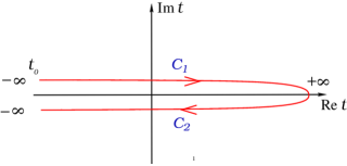
Figure 3.1: The Keldysh path on the time-plane along which the nonequilibrium Green’s function is defined.

One can introduce the so-called Keldysh Green’s function [10] which is defined in the following way

$$G^{K}_{{\bf qp}\sigma}(t,t^{\prime})=2i\langle a^{\dagger}_{{\bf p}\sigma}(t^{\prime})b_{{\bf q}\sigma}(t)\rangle.$$ (3.7)

The Keldysh Green’s function (3.7) is a part of a general path-ordered Green’s function

$$G_{{\bf pq}\sigma}(t,t^{\prime})=-i\langle T_{C}\;b_{{\bf q}\sigma}(t)a^{\dagger}_{{\bf p}\sigma}(t^{\prime})\rangle,$$ (3.8)

which is defined on a so-called Keldysh contour $C=C_{1}+C_{2}$ showed in Fig. 3.1, $T_{C}$ is a time-ordering operator along this contour. It is convenient to separate the Keldysh contour on the upper ($C_{1}$) and lower ($C_{2}$) contours and to present the function (3.8) in a matrix form

$$\hat{G}=\left(\begin{array}[]{cc}G_{11}&G_{12}\\ G_{21}&G_{22}\end{array}\right),$$ (3.9)

where indices $1$ and $2$ refer to the upper or lower Keldysh contour respectively. By applying the usual rotation operator

$$R=\frac{1}{\sqrt{2}}\left(\begin{array}[]{cc}1&1\\ -1&1\end{array}\right)$$ (3.10)

to the matrix (3.9): $\hat{G}\rightarrow R^{-1}\hat{G}R$ we get the nonequilibrium Green’s function in the Larkin-Ovchinnikov representation [12]

$$\hat{G}=\left(\begin{array}[]{cc}G^{R}&G^{K}\\ 0&G^{A}\end{array}\right).$$ (3.11)

The relation between $G_{11}$, $G_{12}$, $G_{21}$, $G_{22}$ and retarded $G^{R}$, advance $G^{A}$ and Keldysh $G^{K}$ Green’s functions can be trivially derived from (3.9) and (3.10). For details see [10, 11].

The Keldysh Green’s function (3.7) is useful, because we can immediately express the current (3.6) in terms of such functions

$$I=-\frac{e}{2\hbar}\sum_{{\bf pq}\sigma}\left(T_{{\bf pq}}G^{K}_{{\bf qp}\sigma}(t)-T_{{\bf pq}}^{*}G^{K}_{{\bf pq}\sigma}(t)\right).$$ (3.12)

One can readily see that $[G^{K}_{{\bf pq}\sigma}(t)]^{*}=-G^{K}_{{\bf qp}\sigma}(t)$, so that the expression for the current becomes even simpler

$$I=-\frac{e}{\hbar}Re\left[\sum_{{\bf pq}\sigma}T_{{\bf pq}}G^{K}_{{\bf qp}\sigma}(t)\right].$$ (3.13)

We need thus to calculate the Keldysh Green’s function $G^{K}_{{\bf qp}\sigma}(t)$. For simplicity we proceed with our calculations in the first order of perturbation theory. We also consider only $G_{{\bf pq}\uparrow}$ function, because $G_{{\bf pq}\downarrow}$ can be derived analogously.

The Green’s function of the system described by the Hamiltonian (3.1) in the first order of perturbation theory reads

$$G^{(1)}_{{\bf pq}\uparrow}(t,t^{\prime})=-i\langle T_{C}\left(1-i\int_{C}d\tau H_{T}(\tau)\right)b_{{\bf q}\uparrow}(t)a^{\dagger}_{{\bf p}\uparrow}(t^{\prime})\rangle.$$ (3.14)

According to the BCS theory only electrons with opposite momenta and spins are allowed to pair, hence we get the expression

$$G^{(1)}_{{\bf pq}\uparrow}(t,t^{\prime})=T_{\bf-p,-q}\langle T_{C}\int_{C}d\tau b_{{\bf q}\uparrow}(t)b_{-{\bf q}\downarrow}(\tau)a^{\dagger}_{-{\bf p}\downarrow}(\tau)a^{\dagger}_{{\bf p}\uparrow}(t^{\prime})\rangle.$$ (3.15)

We assume, that in the simplest approximation the critical supercurrent is carried by Cooper pairs, and by applying Wick’s theorem [13] to (3.15) we get

$$G^{(1)}_{{\bf pq}\uparrow}(t,t^{\prime})=-T_{\bf-p,-q}\int_{C}d\tau\,\mathcal{F}_{\uparrow\downarrow}({\bf q},t-\tau)\overline{\mathcal{F}}_{\downarrow\uparrow}({\bf p},\tau-t^{\prime}).$$ (3.16)

Here we introduced anomalous Gor’kov functions for a superconductor [13]

$$\mathcal{F}_{\uparrow\downarrow}({\bf q},t-t^{\prime}) = -i\langle T_{C}\,b_{{\bf q}\uparrow}(t)b_{-{\bf q}\downarrow}(t^{\prime})\rangle$$

$$\overline{\mathcal{F}}_{\downarrow\uparrow}({\bf p},t-t^{\prime}) = -i\langle T_{C}\,a_{-{\bf p}\downarrow}^{\dagger}(t)a_{{\bf p}\uparrow}^{\dagger}(t^{\prime})\rangle.$$ (3.17)

These Green’s function do not depend on the sign of momentum ${\bf p}$, but the order of spin indices does matter (replacing $\uparrow\downarrow$ with $\downarrow\uparrow$ will give an extra minus sign).

In a lengthy but straightforward calculation [11] one can extract the Keldysh part of the matrix Green’s function (3.16)

$$[G^{(1)}_{{\bf pq}\uparrow}(t,t^{\prime})]^{K}=-T_{pq}^{*}\int_{-\infty}^{\infty}d\tau[\mathcal{F}_{\uparrow\downarrow}^{R}({\bf q},t-\tau)\overline{\mathcal{F}}^{K}_{\downarrow\uparrow}({\bf p},\tau-t^{\prime})+\mathcal{F}_{\uparrow\downarrow}^{K}({\bf q},t-\tau)\overline{\mathcal{F}}^{A}_{\downarrow\uparrow}({\bf p},\tau-t^{\prime})],$$ (3.18)

The Fourier transformation of this expression gives

$$[G^{(1)}_{{\bf pq}\uparrow}(\omega)]^{K}=-T_{pq}^{*}[\mathcal{F}_{\uparrow\downarrow}^{R}({\bf q},\omega)\overline{\mathcal{F}}^{K}_{\downarrow\uparrow}({\bf p},\omega)+\mathcal{F}_{\uparrow\downarrow}^{K}({\bf q},\omega)\overline{\mathcal{F}}^{A}_{\downarrow\uparrow}({\bf p},\omega)].$$ (3.19)

The current then becomes

$$I=\frac{2e}{\hbar}Re\left[\sum_{{\bf pq}}|T_{{\bf pq}}|^{2}\int_{0}^{\infty}\frac{d\omega}{2\pi}\left(\mathcal{F}_{\uparrow\downarrow}^{R}({\bf q},\omega)\overline{\mathcal{F}}^{K}_{\downarrow\uparrow}({\bf p},\omega)+\mathcal{F}_{\uparrow\downarrow}^{K}({\bf q},\omega)\overline{\mathcal{F}}^{A}_{\downarrow\uparrow}({\bf p},\omega)\right)\right],$$ (3.20)

the factor of “2” appears because the contribution from $G^{K}_{{\bf pq}\downarrow}$ is equivalent to the contribution from $G^{K}_{{\bf pq}\uparrow}$.

This expression simplifies greatly in equilibrium, in which case the Keldysh Green’s function can be expressed as

$$G^{K}(\omega)=(G^{R}(\omega)-G^{A}(\omega))(1-2f(\omega)),$$ (3.21)

where $f(\omega)=(e^{\omega/T}+1)^{-1}$ is the Fermi distribution function. Hence we get

$$I=\frac{2e}{\hbar}Re\left[\sum_{{\bf pq}}|T_{{\bf pq}}|^{2}\int_{0}^{\infty}\frac{d\omega}{2\pi}\tanh\left(\frac{\omega}{2T}\right)\left(\mathcal{F}_{\uparrow\downarrow}^{R}({\bf q},\omega)\overline{\mathcal{F}}^{R}_{\downarrow\uparrow}({\bf p},\omega)-\mathcal{F}_{\uparrow\downarrow}^{A}({\bf q},\omega)\overline{\mathcal{F}}^{A}_{\downarrow\uparrow}({\bf p},\omega)\right)\right].$$ (3.22)

Substituting the explicit expressions for the retarded and the advanced Gor’kov functions [13] we obtain

$$I = \frac{2e}{\hbar}Re\Big{[}\sum_{{\bf pq}}|T_{{\bf pq}}|^{2}\int_{0}^{\infty}\frac{d\omega}{2\pi}\tanh\left(\frac{\omega}{2T}\right)\Big{(}\frac{-\Delta_{\bf q}}{(\omega+i\delta)^{2}-\epsilon_{\bf q}^{2}-|\Delta_{\bf q}|^{2}}\frac{-\Delta_{\bf p}^{*}}{(\omega+i\delta)^{2}-\epsilon_{\bf p}^{2}-|\Delta_{\bf p}|^{2}}$$ (3.23)

$$- \frac{-\Delta_{\bf q}}{(\omega-i\delta)^{2}-\epsilon_{\bf q}^{2}-|\Delta_{\bf q}|^{2}}\frac{-\Delta_{\bf p}^{*}}{(\omega-i\delta)^{2}-\epsilon_{\bf p}^{2}-|\Delta_{\bf p}|^{2}}\Big{)}\Big{]}.$$

We assume that superconducting gaps in the left and right leads are momentum-independent $\Delta_{\bf q}\equiv\Delta_{1}$ and $\Delta_{\bf p}\equiv\Delta_{2}$, and their product gives $\Delta_{1}\Delta_{2}^{*}=|\Delta_{1}||\Delta_{2}|e^{i\phi}$, where $\phi$ is the phase difference between two superconductors. We also take into account that the integrand is purely imaginary, so that the current becomes

$$I = \frac{2e}{\hbar}|\Delta_{1}||\Delta_{2}|(i\sin(\phi))\Big{[}\sum_{{\bf pq}}|T_{{\bf pq}}|^{2}\int_{0}^{\infty}\frac{d\omega}{2\pi}\Big{(}\frac{1}{(\omega+i\delta)^{2}-\epsilon_{\bf q}^{2}-|\Delta_{1}|^{2}}\frac{1}{(\omega+i\delta)^{2}-\epsilon_{\bf p}^{2}-|\Delta_{2}|^{2}}$$ (3.24)

$$- \frac{1}{(\omega-i\delta)^{2}-\epsilon_{\bf q}^{2}-|\Delta_{1}|^{2}}\frac{1}{(\omega-i\delta)^{2}-\epsilon_{\bf p}^{2}-|\Delta_{2}|^{2}}\Big{)}\tanh\left(\frac{\omega}{2T}\right)\Big{]}.$$

We thus derived microscopically that the current between two superconductors is proportional to $\sin\phi$

$$I=I_{c}\sin\phi,$$ (3.25)

where $I_{c}$ is the critical supercurrent

$$I_{c} = \frac{2ie}{\hbar}|\Delta_{1}||\Delta_{2}|\sum_{{\bf pq}}|T_{{\bf pq}}|^{2}\int_{0}^{\infty}\frac{d\omega}{2\pi}\Big{(}\frac{1}{(\omega+i\delta)^{2}-\epsilon_{\bf q}^{2}-|\Delta_{1}|^{2}}\frac{1}{(\omega+i\delta)^{2}-\epsilon_{\bf p}^{2}-|\Delta_{2}|^{2}}$$ (3.26)

$$- \frac{1}{(\omega-i\delta)^{2}-\epsilon_{\bf q}^{2}-|\Delta_{1}|^{2}}\frac{1}{(\omega-i\delta)^{2}-\epsilon_{\bf p}^{2}-|\Delta_{2}|^{2}}\Big{)}\tanh\left(\frac{\omega}{2T}\right).$$

Using standard rules of contour integration we can replace the integral over $\omega$ by a sum over discrete Matsubara frequencies $\omega_{n}=(2n+1)\pi T$ [9]

$$I_{c}=\frac{4e}{\hbar}|\Delta_{1}||\Delta_{2}|T\sum_{\bf pq}|T_{{\bf pq}}|^{2}\sum_{n=-\infty}^{\infty}\frac{1}{\omega_{n}^{2}+\epsilon_{\bf q}^{2}+|\Delta_{1}|^{2}}\frac{1}{\omega_{n}^{2}+\epsilon_{\bf p}^{2}+|\Delta_{2}|^{2}}.$$ (3.27)

The summation over ${\bf p}$ and ${\bf q}$ can be replaced by an integral, which can be taken

$$I_{c}=\frac{4\pi^{2}e}{\hbar}|\Delta_{1}||\Delta_{2}|N_{1}(0)N_{2}(0)\;|T_{0}|^{2}\;T\sum_{n=-\infty}^{\infty}\frac{1}{\sqrt{\omega_{n}^{2}+\Delta_{1}^{2}}}\frac{1}{\sqrt{\omega_{n}^{2}+\Delta_{2}^{2}}},$$ (3.28)

where $N_{1}(0)$ and $N_{2}(0)$ are the densities of states at the Fermi energy in the normal state of left and right lead correspondingly. When the two gaps are equal to each other $\Delta_{1}=\Delta_{2}\equiv\Delta$, this expression takes a simple form

$$I_{c}=\frac{2\pi^{2}e}{\hbar}\Delta\;N_{1}(0)N_{2}(0)\;|T_{0}|^{2}\tanh\left(\frac{\Delta}{2T}\right).$$ (3.29)

One usually introduces the so-called resistance of the tunneling junction in the normal state $R_{n}$

$$\frac{1}{R_{n}}=4\pi e^{2}N_{1}(0)N_{2}(0)\;|T_{0}|^{2},$$ (3.30)

so that

$$I_{c}R_{n}=\frac{\pi\Delta}{2e}\tanh\left(\frac{\Delta}{2T}\right).$$ (3.31)

In Fig. 3.2 we depict the temperature behavior of the Josephson critical current $I_{c}$, normalized by $\pi T_{c}/2eR_{n}$. In order to obtain this dependence we had to solve the standard BCS gap equation, and we present the temperature dependence of the gap in the same Fig. One can see, that the critical current is monotonously decreasing with temperature rather similar to the gap behavior. Near $T_{c}$ the current is proportional to $\Delta^{2}$ and is therefore linear in $(T_{c}-T)$.

At zero temperature the critical supercurrent for superconductors with different gaps is

$$I_{c}^{0}=\frac{2\Delta_{1}(0)\Delta_{2}(0)}{eR[\Delta_{1}(0)+\Delta_{2}(0)]}K\left(\frac{|\Delta_{1}(0)-\Delta_{2}(0)|}{\Delta_{1}(0)+\Delta_{2}(0)}\right),$$ (3.32)

where $K(x)$ is a complete elliptic integral of the first kind. In case of $\Delta_{1}(0)=\Delta_{2}(0)\equiv\Delta_{0}$ we get a simple expression

$$I_{c}^{0}R_{n}=\frac{\pi}{2e}\Delta_{0}.$$ (3.33)

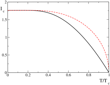
Figure 3.2: Josephson critical current defined by Eq. (3.31) in the units of $\pi T_{c}/2eR_{n}$ (solid line). The dashed line shows the temperature dependence of the BCS gap $\Delta/T_{c}$.

Chapter 4 Josephson effect in Bose-Einstein condensates

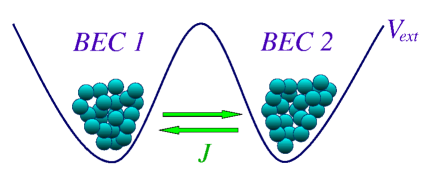
Figure 4.1: Bose Josephson junction: two Bose-Einstein condensates are trapped in an external double-well potential $V_{ext}$.

Condensates of cold alkali atoms [14, 15] provide a unique opportunity to realize and to control Josephson effect in a weakly interacting bosonic system. It was first predicted in [16]. A weak link between two condensates can be realized in a double-well external potential $V_{ext}$ (Fig. 4.1). An interacting system of bosons confined in such a potential is described by a general Hamiltonian

$$H = \int d{\bf r}\;\hat{\Psi}^{\dagger}({\bf r},t)\left[-\frac{\hbar^{2}}{2m}\triangledown^{2}+V_{ext}({\bf r})\right]\hat{\Psi}({\bf r},t)$$ (4.1)

$$+ \frac{1}{2}\int d{\bf r}\int d{\bf r^{\prime}}\hat{\Psi}^{\dagger}({\bf r},t)\hat{\Psi}^{\dagger}({\bf r^{\prime}},t)V({\bf r}-{\bf r^{\prime}})\hat{\Psi}({\bf r^{\prime}},t)\hat{\Psi}({\bf r},t).$$

Here $\hat{\Psi}({\bf r},t)$ is the bosonic field operator and $V({\bf r}-{\bf r^{\prime}})$ is a two-particle interaction.

At low temperatures an experimentally realized gas of bosons is very dilute and particles are weakly interacting, one can therefore introduce a contact interaction between the particles

$$V({\bf r}-{\bf r^{\prime}})=g\delta({\bf r}-{\bf r^{\prime}}),$$ (4.2)

where $g=4\pi\hbar^{2}a_{s}/m$ with $a_{s}$ being the $s-$wave scattering length. According to the Bogoliubov approximation one can consider the bosonic field operator as a sum of a classical field (condensate wave function, representing the condensate order parameter) and excitations

$$\hat{\Psi}({\bf r},t)=\Psi({\bf r},t)+\delta\hat{\Psi}({\bf r},t).$$ (4.3)

In the mean-field description we can neglect the excitations due the smallness of the interaction term, so that our Hamiltonian becomes essentially classical

$$H=\int d{\bf r}\;\Psi^{\dagger}({\bf r},t)\left[-\frac{\hbar^{2}}{2m}\triangledown^{2}+V_{ext}({\bf r})\right]\Psi({\bf r},t)+\frac{g}{2}\int d{\bf r}\Psi^{\dagger}({\bf r},t)\Psi^{\dagger}({\bf r},t)\Psi({\bf r},t)\Psi({\bf r},t).$$ (4.4)

For the Josephson effect to occur only a small overlap of the condensate wave-functions is sufficient, and we can assume that the condensate wave-function $\Psi({\bf r},t)$ is given by the sum of the order parameters for each well [17]

$$\Psi({\bf r},t)=\Psi_{1}({\bf r},t)+\Psi_{2}({\bf r},t)=\varphi_{1}({\bf r})\psi_{1}(t)+\varphi_{2}({\bf r})\psi_{2}(t).$$ (4.5)

Here $\varphi_{1}({\bf r})$ and $\varphi_{2}({\bf r})$ are the ground state solutions for isolated traps [17, 18], and

$$\psi_{i}(t)=N_{i}(t)e^{i\phi_{i}(t)}$$ (4.6)

is the complex condensate order parameter with $N_{i}$ being the number of particles in the $i$-th well, and $\phi_{i}$ is the phase of the condensate in the same well. With these notations the Hamilton function (4.4) takes the form

$$H=E_{1}N_{1}+E_{2}N_{2}+\frac{U_{1}}{2}N_{1}^{2}+\frac{U_{2}}{2}N_{2}^{2}+2J\sqrt{N_{1}N_{2}}\cos(\phi),$$ (4.7)

where $\phi$ is the phase difference between the wells,

$$U_{i} = g\int d{\bf r}|\varphi_{i}|^{4},$$ (4.8)

$$E_{i} = \int d{\bf r}\left(\frac{\hbar^{2}}{2m}|\triangledown\varphi_{i}({\bf r})|^{2}+\varphi_{i}^{2}({\bf r})V_{ext}({\bf r})\right),$$ (4.9)

and $J$ is the Josephson coupling

$$J=-\int d{\bf r}\left(\frac{\hbar^{2}}{2m}\triangledown\varphi_{1}({\bf r})\triangledown\varphi_{2}({\bf r})+\varphi_{1}({\bf r})\varphi_{2}({\bf r})V_{ext}({\bf r})\right).$$ (4.10)

One can reexpress the Hamiltonian (4.7) in terms of a particle imbalance $n$

$$n=\frac{N_{1}-N_{2}}{N_{1}+N_{2}}$$ (4.11)

so that the effective (dimensionless) Josephson Hamiltonian reads

$$H=\frac{\Lambda}{2}n^{2}-\sqrt{1-n^{2}}\cos\phi+\Delta E\;n.$$ (4.12)

We see that in this case only two parameters determine the behavior of the system: the effective interaction

$$\Lambda=(U_{1}+U_{2})(N_{1}+N_{2})/(4J)$$ (4.13)

and the effective chemical potential difference

$$\Delta E=\frac{E_{1}-E_{2}}{2J}+\frac{(U_{1}-U_{2})(N_{1}+N_{2})}{4J}.$$ (4.14)

As the particle number operator $\hat{n}$ and phase operator $\hat{\phi}$ are canonically conjugated variables, in the classical case one can identify a corresponding Poisson bracket with their commutator. We can then derive the corresponding equations of motion for the particle imbalance and phase difference

$$\dot{n}=-\frac{\partial H}{\partial\phi},\quad\dot{\phi}=\frac{\partial H}{\partial n}.$$ (4.15)

As a result we get

$$\dot{n} = -\sqrt{1-n^{2}}\sin\phi,$$ (4.16)

$$\dot{\phi} = \Lambda n+\Delta E+\frac{n}{\sqrt{1-n^{2}}}\cos\phi.$$ (4.17)

These equations can be solved exactly in terms of the elliptic functions [20]. In Fig. 4.2 we show the numerical solutions of the equations (4.17) for $\Delta E=0$. One can observe a qualitative change in the oscillations after $\Lambda$ exceeds a certain “crossover” value $\Lambda_{c}$. For initial conditions as in Fig. 4.2 $\Lambda_{c}\sim 10$. For $\Lambda<\Lambda_{c}$ the time-average of the particle imbalance is zero: $\langle n\rangle_{t}=0$. For larger values of $\Lambda$ the particle imbalance oscillates around a finite value (in case of Fig. 4.2 $\langle n\rangle_{t}=0.4$). It means that on average the number of particles in one well is larger than the number of particles in the other well. This curious quantum phenomenon was termed macroscopic quantum self-trapping (MST) [17]. This behavior can be also seen in a phase portrait in Fig.4.3, showing the constant energy trajectories for different $\Lambda$. The “running” trajectories (c) and (d) correspond to MST.

Figure 4.2: Temporal oscillations of the particle imbalance $n$ and phase difference $\phi$ for $\Lambda=5$ (a), $\Lambda=9$ (b), and $\Lambda=11$ (c). Initially $n(0)=0.6$ and $\phi(0)=0$.

The occurrence of the MST phenomenon is readily understood if one remembers that the canonical Josephson Hamiltonian (4.12) in the small $n$ limit

$$H=\frac{\Lambda}{2}n^{2}-\cos\phi+\Delta E\;n$$ (4.18)

can be mapped onto a pendulum Hamiltonian with tilt angle $\phi$, dimensionless angular momentum $p_{\phi}=n$, inverse mass $\Lambda$ and applied torque $\Delta E$ [15]. For small $n$ the bosonic junction supports small-amplitude Josephson “plasma” oscillations with the frequency $\omega=\sqrt{\Lambda}/(2J)$ Fig. 4.4(a). A rotation of the pendulum in Fig. 4.4(b) corresponds to the MST-state with a running phase. It is also easy to understand the “wiggles” in the phase dynamics in Fig. 4.2 (c), as the pendulum always slows down at its highest point.

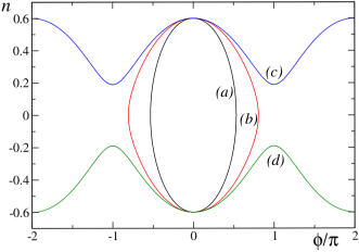
Figure 4.3: Phase space plot: (a), (b) and (c) for same parameters as in Fig.4.2, (d) is for $\Lambda=11$, $n(0)=-0.6$, $\phi(0)=2\pi$.

Figure 4.4: Analogy with pendulum oscillations: MST state corresponds to the case (b), while standard Josephson oscillations of a bosonic junction to the case (a).

The physical behavior of the Bose Josephson junction described by the Hamiltonian (4.12) is more complicated due to the additional factor $\sqrt{1-n^{2}}$. In the language of pendulum analogy it means that the length of the pendulum is not rigid anymore, but varies with time. This leads to additional fixed points in comparison with the previous, simple example (for a detailed description see [20, 19]).

The value of $\Lambda_{c}$ which determines the crossover to the MST state is defined by the condition

$$H_{0}\equiv H(n(0),\phi(0))=\frac{\Lambda}{2}n(0)^{2}-\sqrt{1-n(0)^{2}}\cos(\phi(0))>1,$$ (4.19)

so that

$$\Lambda_{c}=2\frac{1+\sqrt{1-n(0)^{2}}\cos(\phi(0))}{n(0)^{2}}.$$ (4.20)

It means that $\Lambda_{c}$ can be relatively easy controlled in an experiment by varying the initial conditions for two condensates. This property was used by experimentalists and the predicted in [17] behavior of the Bose Josephson junction was successfully observed experimentally [21]. Josephson oscillations of the particle imbalance with $\langle n\rangle_{t}=0$ were observed for $n(0)\approx 0.28(6)$ and $\phi(0)\approx 0$. The MST regime was achieved with $n(0)\approx 0.62(6)$ and $\phi(0)\approx 0$, the parameter $\Lambda$ in both cases is estimated to have a fixed value of $15(3)$.

The analogue of a.c. and d.c. Josephson effect discussed for superconductors in Section 2 has been recently observed in a Bose Josephson junction [22].

Chapter 5 Josephson effect in superfluid He

Since superfluid Helium possesses phase rigidity, one would expect the Josephson effect to occur between two weakly coupled Helium systems. Although liquid Helium was discovered more than seventy years ago (in 1937 by P. Kapitsa, J. F. Allen and D. Misener), it took a long time before the Josephson effect has been finally observed: in 1997 in superfluid ³He [23] and in 2001 in ⁴He [24]. The main obstacle for the observation of the effect is a very small coherence (healing) length of Helium: $50$ nm for ³He and even smaller, of the order of $0.1$ nm for ⁴He. It took thus almost 60 years to overcome two main technical difficulties: (i) the creation of the weak link itself - a structure with small apertures with dimensions of the scale of the coherence length, (ii) measurement of tiny mass currents which would flow through such a structure due to the Josephson effect.

Note, that in case of liquid Helium, one can not apply an external electromagnetic potential difference to the system, as in the case of superconductors, neither can one modify the trapping potential to simulate this effect as in Bose-Einstein condensates of cold atoms. For Helium the role of external potential $V$ is played by pressure $P$, so that both Josephson relations (2.21) and (2.22) remain the same with chemical potential difference proportional to pressure:

$$\Delta\mu=\frac{\Delta Pm}{\rho}.$$ (5.1)

Here $m$ is the mass of either the ⁴He atom, or twice the ³He atomic mass (³He is a fermionic system and its superfluidity is induced by coupled fermions), $\rho$ is the liquid density. Applied pressure difference will induce therefore an oscillating mass supercurrent with the frequency $\omega_{f}=\Delta Pm/\rho h$.

In the experiment [23] two ³He systems are separated by a membrane with numerous apertures only 100 nm in diameter. The healing length at the given experimental temperature was slightly exceeding the aperture diameter. The great number of apertures (more than 4000) served to coherently increase the monitored supercurrent, which was otherwise too tiny to be resolve in the measurement. Another soft membrane controlled by an applied bias was used in order to create an external pressure difference. Any displacements of the membrane due to the supercurrent were monitored. Finally, the signals of the supercurrent frequency obtained in this way were amplified and connected to audio head-phones, and the listener could literally hear the effect of coherent quantum oscillations between weakly coupled superfluids. It sounded like a whistle smoothly drifting from high to low frequency while the pressure relaxed to its zero value. The dependence of the supercurrent frequency on $\Delta P$ has been found to be perfectly linear [23].

In ⁴He the regime of ordinary Josephson oscillations across an aperture was for a long time believed to be unobservable due to the strong fluctuations of the order parameter in the volume with dimensions of the order of coherence length. In the experiment, however, all the difficulties have been recently overcome and a clear, unsmeared signature of Josephson oscillations has been found [24].

Chapter 6 Outlook

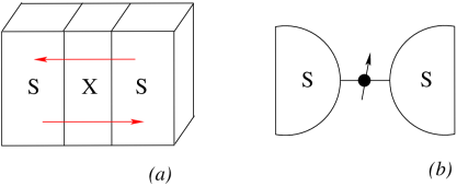
Figure 6.1: Two examples of mesoscopic structures in which Josephson effect plays a role: heterostructure with a normal or ferromagnetic layer embedded between two superconductors: X=N,FM (a); or a quantum dot coupled to superconducting leads (b).

The Josephson effect, predicted and discovered in the 1960-s in superconducting systems, opened a broad avenue of a new research area related to this phenomenon, which is still very active. It is impossible to mention in a short review all the interesting subfields which deal in one or another way with the Josephson phenomena. We give therefore just a few examples.

In addition to the contributions due to Cooper pair tunneling discussed in Section 2, one should take into account quasi-particle terms [2], which we did not consider. Those contributions are especially important for the nonstationary Josephson effect, i.e. in case of the finite voltage applied to the junction. Many other effects influence the behavior of the particle tunneling between two superconductors: various impurities, magnetic fields, inhomogeneities, different pairing symmetries [2, 8].

Many interesting phenomena arise due to the so-called proximity effect [25]: superconductivity penetrates up to a certain length scale into the neighboring normal, or ferromagnetic material (X=N,FM as in Fig. 6.1(a)). In the case of S-X-S heterostructure, shown in Fig. 6.1(a) the layer between two superconductors does not need to be very thin for a supercurrent to occur (for reviews see [25, 26, 27, 28]). Due to the new experimental discoveries in superfluid Helium [23, 24], the question arises whether an equivalent of an S-N-S structure can be created also in these systems.

Another interesting system is a quantum dot coupled to two superconducting leads shown in Fig. 6.1(b) (for review on the transport through quantum dots see for instance [29]). One can consider a similar arrangement in a bosonic system [30].

Finally, a fundamental physical problem is a nonequilibrium Josephson effect. For example, in a bosonic system it is easily realized, as the barrier between the two wells confining condensates is ramped up in a nonadiabatic way [21]. This gives rise to quasi-particle excitations out of the condensate [31, 32]. One can then develop a description in terms of the Keldysh Green’s functions [32], which we mentioned in the context of the superconducting Josephson junction in Section 2.

Bibliography

- [1] B. D. Josephson, Phys. Lett. 1, 251 (1962).
- [2] A. Barone, G. Paterno, Physics and Applications of the Josephson Effect, John Wiley and Sons, New York (1982).
- [3] P. W. Anderson, J. Chem. Phys. Solids 11, 26 (1959).
- [4] A. A. Abrikosov, Fundamentals of the Theory of Metals, North Holland, Amsterdam, Oxford, New York, Tokio, 1988.
- [5] R. P. Feynman, R. B. Leighton, and M. Sands. The Schrödinger equation in a classical context: A seminar on superconductivity. In The Feynman Lectures on Physics, Vol. III, Addison-Wesley (1965).
- [6] P. W. Anderson, Ravello-Lectures on the Many-Body Problem. 2, Ed. E. R. Gaianello, Acad. Press, p. 115 (1963).
- [7] V. Ambegaokar, and A. Baratoff, Phys. Rev. Lett. 10, 486 (1963), ibid 11, 104 (1963).
- [8] I. O. Kulik and I. K. Yanson, The Josephson effect in superconductive tunneling structures, Jerusalem 1972, translation from the book Effekt DZhozefsona v sverkhprovodyashchikh tunnel’nykh strukturakh, Nauka, Moskva 1970.
- [9] Gerald D. Mahan, Many-Particle Physics, Plenum Press, New York and London, 1990.
- [10] L. V. Keldysh, Zh. Eksp. Teor. Fiz. 47, 1515 (1964) [Sov. Phys.–JETP 20, 1018 (1965)].
- [11] J. Rammer and H. Smith, Rev. Mod. Phys. 58, 323 (1986).
- [12] A. I. Larkin, and Yu. N. Ovchninnikov, Zh. Eksp. Teor. Fiz. 68, 1915 (1975) [Sov. Phys. - JETP 41, 960 (1975)].
- [13] A. A. Abrikosov, L. P. Gor’kov, I. Ye. Dzyaloshinskii, Quantum Field Theoretical Methods in Statistical Physics, Pergamon, (1965).
- [14] F. Dalfovo, S. Giorgini, L. P. Pitaevskii, S. Stringari, Rev. Mod. Phys. 71, 463 (1999).
- [15] A. J. Leggett, Rev. Mod. Phys. 73, 307 (2001).
- [16] J. Javanainen, Phys. Rev. Lett. 57, 3164 (1986).
- [17] A. Smerzi, S. Fantoni, S. Giovanazzi, and S. R. Shenoy, Pys. Rev. Lett. 79, 4950 (1997).
- [18] G. J. Milburn, J. Corney, E. M. Wright, and D. F. Walls, Phys. Rev. A 55, 4318 (1997).
- [19] Subodh R. Shenoy, Pramana 58, 385 (2002).
- [20] S. Raghavan, A. Smerzi, S. Fantoni, and S. Shenoy, Phys. Rev. A 59, 620 (1999)
- [21] M. Albiez, R. Gati, J. Fölling, S. Hunsmann, M. Cristiani, and M. K. Oberthaler, Phys. Rev. Lett. 95, 010402 (2005).
- [22] S. Levy, E. Lahoud, I. Shomroni, and J. Steinhauer, Nature 449, 579 (2007).
- [23] S. V. Pereverzev, A. Loshak, S. Backhaus, J. C. Davis, and R. E. Packard, Nature 388, 449 (1997).
- [24] K. Sukhatme, Y. Mukharsky, T. Chui, and D. Pearson, Nature 411, 280 (2001).
- [25] P.G. de Gennes, Rev. Mod. Phys. 36, 225 (1964).
- [26] A.A. Golubov, M. Yu. Kupriyanov, E. Il’ichev, Rev. Mod. Phys. 76, 411 (2004).
- [27] A. Buzdin, Rev. Mod. Phys. 77, 935 (2005).
- [28] F. S. Bergeret, A. F. Volkov, and K. B. Efetov, Rev. Mod. Phys. 77, 1321 (2005).
- [29] C. W. J. Beenakker, and H. Van Houten, Solid State Physics 44, 1 (1991).
- [30] U. R. Fischer, C. Iniotakis, and A. Posazhennikova, Phys. Rev. A 77, 031602 (R) (2008).
- [31] I. Zapata, F. Sols, and A. J. Leggett, Phys. Rev. A 67, 021603(R) (2003).
- [32] M. Trujillo Martinez, A. Posazhennikova, and J. Kroha, cond-mat preprint 0903.5459 (2009).