Enumerating the basins of infinity of cubic polynomials

Abstract.

We study the dynamics of cubic polynomials restricted to their basins of infinity, and we enumerate topological conjugacy classes with given combinatorics.

1. Introduction

Let $f:{\mathbb{C}}\to{\mathbb{C}}$ be a polynomial of degree 3 with complex coefficients. Its basin of infinity is the open invariant subset

$$X(f)=\{z\in{\mathbb{C}}:f^{n}(z)\to\infty\mbox{ as }n\to\infty\}.$$

In this article, we examine combinatorial topological-conjugacy invariants of the restricted dynamical system $f:X(f)\to X(f)$ and count the number of possibilities for each invariant. We apply results of [DP1] which show that we can use these invariants to classify topological conjugacy classes of pairs $(f,X(f))$ within the space of cubic polynomials. Moreover, when $f$ is in the shift locus, meaning that both of its critical points lie in $X(f)$, these invariants classify conjugacy classes of polynomials $f:{\mathbb{C}}\to{\mathbb{C}}$.

Specifically, we implement an algorithm which counts topological conjugacy classes of cubic polynomials of generic level N, defined by the condition that

$$G_{f}(c_{1})/3^{N}<G_{f}(c_{2})<G_{f}(c_{1})/3^{N-1};$$

here $\{c_{1},c_{2}\}$ is the set of critical points of the polynomial $f$ and

$$G_{f}(z)=\lim_{n\to\infty}\frac{1}{3^{n}}\log^{+}|f^{n}(z)|$$

is the escape-rate function. These generic cubic polynomials are precisely the structurally stable maps in the shift locus [McS] (see also [DP2]). We examine the growth of the number of these stable conjugacy classes as $N\to\infty$.

We begin with an enumeration of the Branner-Hubbard tableaux (or equivalently, the Yoccoz $\tau$-functions) of length $N$, as introduced in [BH2]; see Theorem 2.2. Using the combinatorics of tableaux, we provide an algorithm for computing the number of truncated spines (introduced in [DP1]) for each $\tau$-function; see Theorem 3.1. Finally, we apply the procedure of [DP1] to count the number of generic topological conjugacy classes associated to each truncated spine. The ideas and proofs follow the treatment of cubic polynomials in [BH1], [BH2], [Br], and [BDK].

1.1. Results of the computation.

An implementation of the algorithm was written with Java. We compiled the output in Table 1 to level $N=21$, together with run times (Processor: 2.39GHz Intel Core 2 Duo, Memory: 2 $\times$ 1GB PC2100 DDR 266MHz).

Level	Tau sequences	Trees	Truncated spines	Conjugacy classes	Run time
1	1	1	1	1	0.000
2	2	2	2	2	0.078
3	4	4	4	4	0.062
4	8	8	8	8	0.063
5	16	18	18	19	0.093
6	33	42	42	46	0.079
7	69	103	105	118	0.078
8	144	260	270	318	0.093
9	303	670	718	881	0.094
10	641	1753	1939	2480	0.125
11	1361	4644	5312	7084	0.156
12	2895	12433	14719	20374	0.266
13	6174	33581	41161	59061	0.547
14	13188	91399	115856	172016	1.141
15	28229	250452	328098	503018	2.453
16	60515	690429	933719	1475478	5.515
17	129940	1913501	2668241	4338715	12.500
18	279415		7652212	12785056	27.109
19	601742		22013683	37739184	72.579
20	1297671		63497798	111562926	163.422
21	2802318		183589726	330215133	383.640

Table 1. Enumeration of conjugacy classes to generic level $N=21$, with run times measured in seconds. The tree numbers were computed in [DM].

Levels 17 / 16	Levels 18 / 17	Levels 19 / 18	Levels 20 / 19	Levels 21 / 20
2.941	2.947	2.952	2.956	2.960

Table 2. Computing the growth: ratios of numbers of conjugacy classes at consecutive levels.

1.2. The tree of cubic polynomials.

We can define a tree ${\mathcal{T}}_{conj}$ of conjugacy classes of cubic polynomials in the shift locus as follows. For each generic level $N\geq 1$, let $V(N)$ be a set of vertices consisting of one vertex for each topological conjugacy class. We connect a vertex $v$ in $V(N+1)$ to a vertex $w$ in $V(N)$ by an edge if for each representive $f$ of $v$ and $g$ of $w$, there exists an $\varepsilon>0$ so that the restrictions $f|\{G_{f}>(G_{f}(c_{1})/3^{N-1})-\varepsilon\}$ and $g|\{G_{g}>(G_{g}(c_{1})/3^{N-1})-\varepsilon\}$ are topologically conjugate. In Figure 1, we have drawn this tree ${\mathcal{T}}_{conj}$ to level $N=5$. The growth rate of the number of conjugacy classes as $N\to\infty$ corresponds to a computation of the “entropy” of this tree.

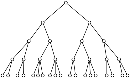
Figure 1. The tree ${\mathcal{T}}_{conj}$ of conjugacy classes to generic level $N=5$.

The tree ${\mathcal{T}}_{conj}$ can also be constructed in the following way. Let $\mathrm{MP}_{3}$ denote the space of conformal conjugacy classes of cubic polynomials; it is a two-dimensional complex orbifold with underlying manifold isomorphic to ${\mathbb{C}}^{2}$. Every cubic polynomial is conformally conjugate to one of the form

$$f(z)=z^{3}+az+b,$$

which can be represented in $\mathrm{MP}_{3}$ by $(a,b^{2})\in{\mathbb{C}}^{2}$.

The critical escape-rate map

$$\mathcal{G}:\mathrm{MP}_{3}\to{\mathbb{R}}^{2}$$

is defined by $\mathcal{G}(f)=(G_{f}(c_{1}),G_{f}(c_{2}))$ where the critical points $\{c_{1},c_{2}\}$ of $f$ are labeled so that $G_{f}(c_{1})\geq G_{f}(c_{2})$; it is continuous and proper [BH1]. The fiber of $\mathcal{G}$ over the origin in ${\mathbb{R}}^{2}$ is the connectedness locus $\mathcal{C}_{3}$, the set of polynomials with connected Julia set. If we restrict $\mathcal{G}$ to its complement $\mathrm{MP}_{3}\setminus\mathcal{C}_{3}$, there is an induced projectivization:

$$\bar{\mathcal{G}}:\mathrm{MP}_{3}\setminus\mathcal{C}_{3}\to[0,1]$$

defined by $f\mapsto G_{f}(c_{2})/G_{f}(c_{1})$. The quotient space of $\mathrm{MP}_{3}\setminus\mathcal{C}_{3}$ formed by collapsing connected components of fibers of $\bar{\mathcal{G}}$ to points is a (completed) tree ${\mathbb{P}}{\mathcal{T}}_{3}^{*}$: over $(0,1]$ it forms a locally finite simplicial tree while $\bar{\mathcal{G}}^{-1}(0)$ forms its space of ends.

In [DP2] it is proved that the edges of the tree ${\mathbb{P}}{\mathcal{T}}_{3}^{*}$ correspond to generic topological conjugacy classes. Thus, the combinatorial tree ${\mathcal{T}}_{conj}$ is dual to the shift locus tree in ${\mathbb{P}}{\mathcal{T}}_{3}^{*}$; each edge in ${\mathbb{P}}{\mathcal{T}}_{3}^{*}$ corresponds to a vertex in ${\mathcal{T}}_{conj}$.

The tree ${\mathbb{P}}{\mathcal{T}}_{3}^{*}$ comes equipped with a projection to the space of cubic trees ${\mathbb{P}}{\mathcal{T}}_{3}$ introduced in [DM]. In [DM] the growth of the number of edges in ${\mathbb{P}}{\mathcal{T}}_{3}$ was studied (see Table 1, third column), but the value of the entropy was left as an open question. Furthermore, the tree ${\mathcal{T}}_{conj}$ is a quotient of the tree of marker autorphisms $\mathcal{M}_{3}$ introduced in [BDK]; the quotient is by the monodromy action from a twisting deformation (see [Br]). The entropy of $\mathcal{M}_{3}$ was easily shown to be $\log 3$, and so the entropy of ${\mathcal{T}}_{conj}$ (or equivalently, of ${\mathbb{P}}{\mathcal{T}}_{3}^{*}$) is no more than $\log 3$.

Question.

Let $\varphi(N)$ denote the number of vertices in ${\mathcal{T}}_{conj}$ at level $N$. Is

$$\lim_{N\to\infty}\frac{1}{N}\log\varphi(N)=\log 3\;?$$

In Table 2, we show the ratios of the number of conjugacy classes in consecutive levels. As the level increases, the computed ratios increase, conjecturally limiting on 3.

2. The $\tau$ functions

2.1. The $\tau$-function of a polynomial.

Fix a cubic polynomial $f$ with disconnected Julia set, and let $c_{1}$ and $c_{2}$ be its critical points, labeled so that $G_{f}(c_{2})\leq G_{f}(c_{1})$. For each integer $n$ such that $G_{f}(c_{2})<G_{f}(c_{1})/3^{n-1}$, we define the critical puzzle piece $P_{n}(f)$ as the connected component of $\{z:G_{f}(z)<G_{f}(c_{1})/3^{n-1}\}$ containing $c_{2}$, and set

$$\tau_{f}(n)=\max\{j<n:f^{n-j}(c_{2})\in P_{j}(f)\}.$$

Recall that the tableau or marked grid of $f$ is an array $\{M_{f}(j,k)\in\{0,1\}:j,k\geq 0\}$, defined by the condition

$$M_{f}(j,k)=1\iff f^{k}(c_{2})\in P_{j}(f).$$

We depict a marked grid as a subset of the 4th quadrant of the ${\mathbb{Z}}^{2}$-lattice, where $j\geq 0$ represents the distance along the negative $y$-axis and $k\geq 0$ respresents the distance along the positive $x$-axis. The values of $\tau_{f}$ can be read directly from the marked grid: beginning with $M_{f}(n,0)=1$, $\tau_{f}(n)$ is the $j$-coordinate at the first non-zero entry when proceeding “northeast” from $(n,0)$. In fact, the orbit $\{\tau_{f}^{k}(n):k\geq 0\}$ consists of the $j$-coordinates of all non-zero entries along the diagonal $M_{f}(n-i,i)$. Thus, the marked grid can be recovered from the $\tau$-function by:

$$M_{f}(j,k)=\left\{\begin{array}[]{ll}1&\mbox{if }j=k=0\\ 1&\mbox{if }j=\tau_{f}^{m}(j+k)\mbox{ for some }m\geq 0\\ 0&\mbox{otherwise}\end{array}\right.$$

Branner and Hubbard [BH2, Theorem 4.1] showed that marked grids associated to cubic polynomials are characterized by a simple set of rules. A marked grid of size $N$ (which may be infinite) is an array $\{M(j,k)\in\{0,1\}:j,k\geq 0\mbox{ and }j+k\leq N\}$ which satisfies the following rules:

• For each $n\leq N$, $M(n,0)=M(0,n)=1$.

• If $M(j,k)=1$, then $M(l,k)=1$ for all $l\leq j$.

• If $M(j,k)=1$, then $M(j-i,k+i)=M(j-i,i)$ for all $0\leq i\leq j$.

• If $j+k<N$, $M(j,k)=1$, $M(j+1,k)=0$, $M(j-i,i)=0$ for $0<i<m$, and $M(j-m+1,m)=1$, then $M(j-m+1,k+m)=0$.

• If $j+k<N$, $M(j,k)=1$, $M(1,j)=0$, $M(j+1,k)=1$, and $M(j-i,k+i)=0$ for all $0<i<j$, then $M(1,j+k)=0$.

The rule (M4) was omitted in [BH2], though it is necessary for their proof. It appears as stated here in [Ki, Proposition 4.5]; an equivalent formulation (in the language of $\tau$-functions) was given in [DM].

2.2. Properties of tau-functions

Let ${\mathbb{N}}$ denote the positive integers $\{1,2,3,\ldots\}$. We consider the following five properties of functions $\tau:{\mathbb{N}}\to{\mathbb{N}}\cup\{0\}$.

• $\tau(1)=0$

• $\tau(n+1)\leq\tau(n)+1$

From (A) and (B), it follows that $\tau(n)<n$ for all $n\in{\mathbb{N}}$; consequently, there exists a unique integer $\operatorname{ord}(n)$ such that the iterate $\tau^{\operatorname{ord}(n)}(n)=0$.

• If $\tau(n+1)<\tau^{k}(n)+1$ for some $0<k<\operatorname{ord}(n)$, then $\tau(n+1)\leq\tau^{k+1}(n)+1$.

• If $\tau(n+1)<\tau^{k}(n)+1$ for some $0<k<\operatorname{ord}(n)$, and if $\tau(\tau^{k}(n)+1)=\tau^{k+1}(n)+1$, then $\tau(n+1)<\tau^{k+1}(n)+1$.

• If $\operatorname{ord}(n)>1$ and $\operatorname{ord}(\tau^{\operatorname{ord}(n)-1}(n)+1)=1$, then $\tau(n+1)\not=0$.

Proposition 2.1.

For any positive integer $N$, a function

$$\tau:\{1,2,3,\ldots,N\}\to{\mathbb{N}}\cup\{0\}$$

or a function

$$\tau:{\mathbb{N}}\to{\mathbb{N}}\cup\{0\}$$

is the $\tau$-function of a cubic polynomial if and only if it satisfies properties (A)–(E).

We say the $\tau$-function is admissible if it satisfies properties (A)–(E).

The proof is by induction on $N$. It is not hard to see that the $\tau$ function must satisfy these rules, by doing a translation of the tableau rules. Conversely, any tau function satisfying properties (A)-(E) determines a marked grid satisfying the 4 tableau rules. Property (E) is another formulation of the “missing tableau rule” (M4) appearing in [Ki] and [DM].

2.3. Algorithm to inductively produce all $\tau$-functions

If a $\tau$-function has domain $\{1,2,3,\ldots,N\}$, we say it has length N. The markers of a $\tau$ with length $N$ are the integers

$$\{m\in\{1,\ldots,N-1\}:\tau(m+1)<\tau(m)+1\}.$$

Let $k$ be the number of markers which appear in the orbit

$$N\mapsto\tau(N)\mapsto\ldots\mapsto\tau^{\operatorname{ord}(N)}(N)=0,$$

and label these $k$ markers by $l_{1}^{\prime},l_{2}^{\prime},\ldots,l_{k}^{\prime}$ so that

$$N=l_{0}^{\prime}>l_{1}^{\prime}>l_{2}^{\prime}>\cdots>l_{k}^{\prime}>0.$$

For each $0\leq i\leq k$, let $l_{i}=\tau(l_{i}^{\prime})$ so that

$$\tau(N)=l_{0}>l_{1}>\cdots>l_{k}\geq 0.$$

Theorem 2.2.

Given an admissible $\tau$-function of length $N$, an extension to length $N+1$ is admissible if and only if

$$\tau(N+1)=l_{i}+1\mbox{ for some }0\leq i\leq k$$

or $\tau(N+1)=0$ if $l_{k}>0$ or $k=0$.

Proof.

The theorem follows from Proposition 2.1. Property (C) implies that $\tau(N+1)$ must be either 0 or of the form $\tau^{k}(N)+1$. Property (D) implies that $\tau(N+1)$ must be either 0 or of the form $l_{i}+1$. Property (E) implies that $\tau(N+1)\not=0$ if $k>0$ and $l_{k}=0$. On the other hand, if $k=0$, both $\tau(N+1)=l_{0}+1=\tau(N)+1$ and $\tau(N+1)=0$ are admissible. ∎

3. The truncated spine

Suppose $f$ is a cubic polynomial of generic level $N$. Introduced in [DP1], the truncated spine of $f$ is a combinatorial object which carries more information than the $\tau$-sequence though it does not generally determine the topological conjugacy class. (It determines the tree of local models for $f$, studied in [DP1].) Here, we describe how to inductively construct truncated spines, and we compute the number of extensions to a truncated spine of length $N+1$ from one of length $N$. We show exactly how many distinct extensions correspond to a choice of $\tau$-function extension.

3.1. The truncated spine of a polynomial

Fix a cubic polynomial $f$ of generic level $N$. The truncated spine is a sequence of $N$ finite hyperbolic laminations, one for each connected component of the critical level sets of $G_{f}$ separating the critical value $f(c_{1})$ from the critical point $c_{2}$, together with a labeling by integers $<N$.

Specifically, beginning with the level $G_{f}(c_{1})$ of fastest-escaping critical point, we identify the level set $\{G_{f}=G_{f}(c_{1})\}$ with the quotient of a metrized circle. The level curve is topologically a figure 8, metrized by its external angles, giving it total length $2\pi$. The critical point $c_{1}$ lies at the singular point of the figure 8, identifying points at distance $2\pi/3$ along a metrized circle. Thus the associated hyperbolic lamination in the unit disk consists of a single hyperbolic geodesic joining two boundary points at distance $2\pi/3$. The lamination is only determined up to rotation. We mark the complementary component in the disk with boundary length $4\pi/3$ with a $0$ to indicate the component of $\{G_{f}<G_{f}(c_{1})\}$ containing the second critical point $c_{2}$.

For each critical level set $\{G_{f}=G_{f}(c_{1})/3^{n}\}$, $0<n<N$, we consider only the connected component which separates $c_{2}$ from $c_{1}$. External angles can be used to metrize the curve, normalizing the angles so the connected curve has total length $2\pi$ for each $n$. The curve can thus be represented as a quotient of a metrized circle; the associated hyperbolic lamination consists of a hyperbolic geodesic joining each pair of identified points. The gaps of the lamination are the connected components of the complement of the lamination in the disk; each gap corresponds to a connected component of $\{G_{f}<G_{f}(c_{1})/3^{n}\}$. A gap in a lamination is labeled by the integer $k\geq 0$ if the corresponding component contains $f^{k}(c_{2})$.

In Figure 2, we provide examples of truncated spines for two polynomials of generic level $N=5$ with the same $\tau$-sequence.

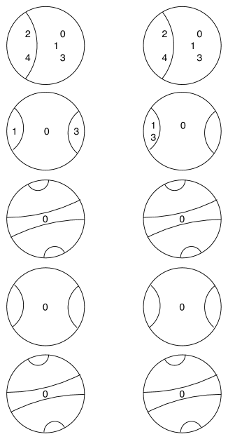
Figure 2. Two truncated spines associated to polynomials of generic level $N=5$ with the same $\tau$-sequence $0,1,0,1,0$.

Two truncated spines of length $N$ are equivalent if for each $0\leq n<N$, the labeled laminations at level $n$ are the same, up to a rotation. In particular, the labeling of the gaps must coincide. It is shown in [DP1] that a truncated spine (together with the heights $(G_{f}(c_{1}),G_{f}(c_{2}))$ of the critical points) determines the full tree of local models for a polynomial of generic level $N$. In particular, it carries more information than the tree of $f$, introduced in [DM], and its $\tau$-function; it does not, however, determine the topological conjugacy class of the polynomial.

The central component of a lamination is the gap containing the symbol $0$; it corresponds to the component containing the critical point $c_{2}$. All non-central gaps are called side components.

3.2. From truncated spine to $\tau$-function

Fix a truncated spine of length $N$. Recall that every $\tau$-function satisfies $\tau(1)=0$. For $N>1$ and each $0<n<N$, we can read $\tau(n)$ directly from the truncated spine by:

$$\tau(n)=\max\{j:\mbox{lamination }j\mbox{ is labeled by }(n-j)\}.$$

To compute $\tau(N)$, we consider the set

$$L(N)=\{j:\mbox{the central component in lamination }j\mbox{ is labeled by }(N-j-1)\}.$$

We then have

$$\tau(N)=\left\{\begin{array}[]{ll}1+\max\{j:j\in L(N)\}&\mbox{ if }L(N)\not=\emptyset\\ 0&\mbox{ if }L(N)=\emptyset\end{array}\right.$$

3.3. Extending a spine of length $N$

Fix a truncated spine of length $N$. It follows directly from the definitions that an extension to length $N+1$ is completely determined by the location of the label $N-\tau(N)$ at level $\tau(N)$. Any choice of central or side component is admissible: it determines the local model for an extended tree of local models (from [DP1]).

The lamination at level $N$ is then constructed by taking a degree 2 branched cover of the lamination at level $\tau(N)$ branched over the gap containing the label $N-\tau(N)$. See [DP1] for a general treatment of branched covers of laminations. The labels are added inductively: for each iterate $1<n\leq\operatorname{ord}(N)$, the label $(N-\tau^{n}(N))$ is placed in the gap at level $\tau^{n}(N)$ which is the image of the gap containing $\tau^{n-1}(N)$ at level $\tau^{n-1}(N)$.

3.4. Computing the number of extended spines for each choice of $\tau(N+1)$

Fix a truncated spine with its $\tau$-function of length $N$. As in §2.3, the markers of $\tau$ are the integers

$$\{m\in\{1,\ldots,N-1\}:\tau(m+1)<\tau(m)+1\}.$$

The marked levels of $\tau$ are all integers in the forward orbits of the markers:

$$\{l\geq 0:l=\tau^{n}(m)\mbox{ for marker }m\mbox{ and }n>0\}\cup\{0\};$$

we say 0 is marked even if there are no markers.

As before, we let $k$ be the number of markers which appear in the orbit

$$N\mapsto\tau(N)\mapsto\ldots\mapsto\tau^{\operatorname{ord}(N)}(N)=0.$$

Label these $k$ markers by $l_{1}^{\prime},l_{2}^{\prime},\ldots,l_{k}^{\prime}$ so that

$$N=l_{0}^{\prime}>l_{1}^{\prime}>l_{2}^{\prime}>\cdots>l_{k}^{\prime}>0.$$

For each $0\leq i\leq k$, let $l_{i}=\tau(l_{i}^{\prime})$ so that

$$\tau(N)=l_{0}>l_{1}>\cdots>l_{k}\geq 0.$$

For each $0\leq i<k$, define $n_{i}$ be the condition that

$$\tau^{n_{i}}(l_{i})=l_{i+1}$$

and define $n_{k}$ so that $\tau^{n_{k}}(l_{k})=0$. For $0<i<j\leq k+1$, we set

$$\delta(i,j)=\left\{\begin{array}[]{ll}1&\mbox{if }\tau(l_{i}^{\prime}+1)=l_{j}+1\\ 0&\mbox{otherwise}\end{array}\right.$$

where by convention we take $l_{k+1}=-1$. Note that $\tau(l_{k}^{\prime}+1)=0$ for every $\tau$, so $\delta(k,k+1)=1$.

At level $l_{0}=\tau(N)$, there are $2^{\operatorname{ord}(l_{0})}=2^{n_{0}+n_{1}+\cdots+n_{k}}$ side components and one central component. Labeling the central component with the integer $(N-\tau(N))$ uniquely corresponds to the choice of $\tau(N+1)=\tau(N)+1$. For each $i>0$, the number of side components which correspond to the choice $\tau(N+1)=l_{i}+1$ is

$$2^{n_{0}}(2^{n_{1}}(2^{n_{2}}(\cdots(2^{n_{i-1}}-\delta(i-1,i))-\cdots)-\delta(2,i))-\delta(1,i));$$

as above, we take $l_{k+1}=-1$. It remains to consider how many distinct truncated spines these side components determine.

The symmetry of $\tau$ is

$$s=\min\{n\geq 0:\tau^{n}(l_{0})\mbox{ is a marked level}\}.$$

Note that $s\leq n_{0}$. To each admissible choice for $\tau(N+1)$ (from Theorem 2.2) we define the $(N+1)$-th spine factor of $\tau$. If $\tau(N+1)=l_{i}+1$, then

$$\operatorname{SF}(\tau,N+1)=\left\{\begin{array}[]{ll}2^{n_{0}-s}(2^{n_{1}}(2^{n_{2}}(\cdots(2^{n_{i-1}}-\delta(i-1,i))-\cdots)-\delta(2,i))-\delta(1,i))&\mbox{if }i>0\\ 1&\mbox{if }i=0\end{array}\right.$$

where, as above, we take $l_{k+1}=-1$. It is now straightforward to see:

Theorem 3.1.

For any $\tau$-function of length $N$, the number of truncated spines with this $\tau$-function is:

$$\operatorname{Spines}(\tau)=\prod_{j=1}^{N}\operatorname{SF}(\tau,j).$$

4. Complete algorithm

We combine the results of the previous sections to produce an algorithm for the complete count of topological conjugacy classes for cubic polynomials with generic level $N$.

Fix a $\tau$-function of length $N$. Recall that the markers of $\tau$ are the integers

$$\{m\in\{1,\ldots,N-1\}:\tau(m+1)<\tau(m)+1\},$$

and the marked levels are:

$$\{l\geq 0:l=\tau^{n}(m)\mbox{ for some }n>0\mbox{ and marker }m\}\cup\{0\};$$

Let $L$ be the number of non-zero marked levels.

For each $n\leq N$, the order of $n$ was defined in §2.2; it satisfies $\tau^{\operatorname{ord}(n)}(n)=0$. For each marked level $l$, compute

$$\operatorname{mod}(l)=\sum_{i=1}^{l}2^{-\operatorname{ord}(i)}$$

and

$$t(l)=\min\{n>0:n\operatorname{mod}(l)\in{\mathbb{N}}\}.$$

The quantity $\operatorname{mod}(l)$ represents the sum of relative moduli of annuli down to level $l$, while $t(l)$ is the numer of twists required to return that marked level to its original configuration. We define

$$T(\tau)=\max\{t(l):l\mbox{ is a marked level}\}$$

or set $T(\tau)=1$ if $\tau$ has no marked levels. The twist factor is defined by

$$\operatorname{TF}(\tau)=\frac{2^{L}}{T(\tau)}.$$

From Theorem 3.1, the number of truncated spines with this $\tau$-function is:

$$\operatorname{Spines}(\tau)=\prod_{j=1}^{N}\operatorname{SF}(\tau,j).$$

By [DP1], the number of topological conjugacy classes associated to $\tau$ is then

$$\operatorname{Top}(\tau)=\operatorname{Spines}(\tau)\cdot\operatorname{TF}(\tau).$$

Combining these computations with Theorem 2.2, it is straighforward to automate an inductive construction of all $\tau$-functions of length $N$, and we obtain an enumeration of all truncated spines and all topological conjugacy classes of generic level $N$.

References

- [BDK] P. Blanchard, R. L. Devaney, and L. Keen. The dynamics of complex polynomials and automorphisms of the shift. Invent. Math. 104(1991), 545–580.
- [Br] B. Branner. Cubic polynomials: turning around the connectedness locus. In Topological methods in modern mathematics (Stony Brook, NY, 1991), pages 391–427. Publish or Perish, Houston, TX, 1993.
- [BH1] B. Branner and J. H. Hubbard. The iteration of cubic polynomials. I. The global topology of parameter space. Acta Math. 160(1988), 143–206.
- [BH2] B. Branner and J. H. Hubbard. The iteration of cubic polynomials. II. Patterns and parapatterns. Acta Math. 169(1992), 229–325.
- [DM] L. DeMarco and C. McMullen. Trees and the dynamics of polynomials. Ann. Sci. École Norm. Sup. 41(2008), 337–383.
- [DP1] L. DeMarco and K. Pilgrim. Escape combinatorics for polynomial dynamics. Preprint, 2009.
- [DP2] L. DeMarco and K. Pilgrim. Critical heights on the moduli space of polynomials. Preprint, 2009.
- [Ki] J. Kiwi. Puiseux series polynomial dynamcs and iteration of complex cubic polynomials. Ann. Inst. Fourier (Grenoble) 56(2006), 1337–1404.
- [McS] C. T. McMullen and D. P. Sullivan. Quasiconformal homeomorphisms and dynamics. III. The Teichmüller space of a holomorphic dynamical system. Adv. Math. 135(1998), 351–395.