PULSAR BINARY BIRTHRATES WITH SPIN-OPENING ANGLE CORRELATIONS

Abstract

One ingredient in an empirical birthrate estimate for pulsar binaries is the fraction of sky subtended by the pulsar beam: the pulsar beaming fraction. This fraction depends on both the pulsar’s opening angle and the misalignment angle between its spin and magnetic axes. The current estimates for pulsar binary birthrates are based on an average value of beaming fractions for only two pulsars, i.e. PSRs B1913+16 and B1534+12. In this paper we revisit the observed pulsar binaries to examine the sensitivity of birthrate predictions to different assumptions regarding opening angle and alignment. Based on empirical estimates for the relative likelihood of different beam half-opening angles and misalignment angles between the pulsar rotation and magnetic axes, we calculate an effective beaming correction factor, $f_{\rm b,eff}$, whose reciprocal is equivalent to the average fraction of all randomly-selected pulsars that point toward us. For those pulsars without any direct beam geometry constraints, we find that $f_{\rm b,eff}$ is likely to be smaller than 6, a canonically adopted value when calculating birthrates of Galactic pulsar binaries. We calculate $f_{\rm b,eff}$ for PSRs J0737-3039A and J1141-6545, applying the currently available constraints for their beam geometry. As in previous estimates of the posterior probability density function P(${\cal R}$) for pulsar binary birthrates ${\cal R}$ , PSRs J0737-3039A and J1141-6545 still significantly contribute to , if not dominate, the Galactic birthrate of tight pulsar-neutron star (NS) and pulsar-white dwarf (WD) binaries, respectively. Our median posterior present-day birthrate predictions for tight PSR-NS binaries, wide PSR-NS binaries , and tight PSR-WD binaries given a preferred pulsar population model and beaming geometry are 89 ${\rm Myr}^{-1}$, 0.5 ${\rm Myr}^{-1}$, and 34 ${\rm Myr}^{-1}$, respectively. For long-lived PSR-NS binaries, these estimates include a weak ($\times 1.6$) correction for slowly decaying star formation in the galactic disk. For pulsars with spin period between 10 ms and 100 ms, where few measurements of misalignment and opening angle provide a sound basis for extrapolation, we marginalized our posterior birthrate distribution P(${\cal R}$) over a range of plausible beaming correction factors. We explore several alternative beaming geometry distributions, demonstrating our predictions are robust except in (untestable) scenarios with many highly aligned recycled pulsars. Finally, in addition to exploring alternative beam geometries, we also briefly summarize how uncertainties in each pulsar binary’s lifetime and in the pulsar luminosity distribution can be propagated into P(${\cal R})$.

1. Introduction

Using pulsar survey selection effects to extrapolate outward to the entire Milky Way, the observed sample of Milky Way field binary pulsars constrains the present-day population and birthrate of these binaries, e.g., Narayan et al. (1991), Phinney (1991), Curran & Lorimer (1995), Kalogera et al. (2001), Kim et al. (2003), henceforth denoted KKL, and references therein. Along with the properties of the population, this empirical birthrate informs models for their formation, e.g., O’Shaughnessy et al. (2008) (hereafter PSC), O’Shaughnessy et al. (2009); detection rate estimates for gravitational-wave observatories like LIGO and VIRGO, e.g. Abbott et al. (2008); and even attempts to unify compact mergers with short $\gamma$-ray bursts (Nakar, 2007). Following KKL, a posterior prediction for the present-day birthrate (${\cal R}$) of pulsar binaries on similar evolutionary tracks to a known pulsar binary can be expressed in terms of the pulsar’s beaming geometry (through the effective beaming correction factor $f_{\rm b,eff}$), effective lifetime $\tau_{\rm eff}$, and the population distribution of individual pulsars (in luminosity and galaxy position, via $N_{psr}$):

$${\cal P}({\cal R})=({\tau_{\rm eff}}/{N_{\rm psr}f_{\rm b,eff}}){\cal R}e^{-({\tau_{\rm eff}}/{N_{\rm psr}f_{\rm b,eff}}){\cal R}}\equiv C{\cal R}e^{-C{\cal R}}$$ (1)

Summing over the individual contributions ${\cal R}_{i}$ from each specific pulsar binary $i$, a posterior prediction for the overall Galactic birthrate is

$${\cal P}({\cal R}_{tot})=\int\Pi~{}d{\cal R}_{i}{\cal P}_{i}({\cal R}_{i})~{}\delta({\cal R}_{tot}-\sum{\cal R}_{i})~{}.$$ (2)

As of 2009, the best constrained $f_{\rm b}$’s for binary pulsars are available for PSRs B1913+16 and B1534+12 (Kalogera et al., 2001). Previous works taking an empirical approach relied on these two pulsars for the beaming correction to the rate estimates, e.g. KKL, Kalogera et al. (2004), Kim et al. (2006) (hereafter KKL06). The average value of $f_{\rm b}\sim 6$ based on PSRs B1913+16 and B1534+12 was used as ‘canonical’ value in order to calculate the birthrate (or merger rate) of pulsar binaries and the inferred detection rates for the gravitational-wave detectors.

The motivation for this paper is to provide not only updated Galactic birthrates of pulsar binaries, but also to provide and explain more generic beaming correction factors for use in the birthrate estimates. In this work, we introduce an empirically-motivated beaming model, derive a probability distribution function for $f_{\rm b}$, and calculate the effective beaming correction factor $f_{\rm b,eff}$ for two types of pulsar binaries, a pulsar with a neutron star (PSR-NS) or a white dwarf (PSR-WD) companion. Specifically, we adopt currently available constraints on a misalignment angle $\alpha$ between pulsar spin and magnetic axes, e.g., Gil & Han (1996), Zhang et al. (2003), Kolonko et al. (2004), as well as the empirical relationship betwen the half-opening angle $\rho$ and pulsar spin period $P_{s}$ as priors (e.g. Kramer et al. 1998). For mildly recycled pulsars ($10~{}{\rm ms}<P_{s}<100~{}{\rm ms}$), we anchor our theoretical expectations with observational bias; see §2 for details.

2. Rate constraints for pulsar binaries

Following KKL, we assume each pulsar $i$ in a pulsar binary is equally visible throughout its effective lifetime $\tau_{i}$ everywhere along a fraction $f_{b,i}$ of all lines of sight from the pulsar, ignoring any bias introduced through time evolution of luminosity and opening angle. Consistent with observations of the Milky Way’s star formation history (Gilmore, 2001), we also assume the star formation rate and pulsar birthrate is constant over the past $\tau_{mw}=10~{}{\rm Gyr}$. Based on these two approximations, the mean number $\bar{N}_{i}$ of pulsars on the same evolutionary track as $i$ that are visible at present can be related to its birthrate ${\cal R}_{i}$ by

$$\bar{N}_{i}=f_{\rm b}^{-1}{\cal R}_{i}\tau_{i}$$ (3)

Conversely, Eq. (3) and Bayesian Poisson statistics uniquely determine our posterior prediction for each pulsar’s birthrate shown in Eq.  (1).

2.1. Number of pulsars

When inverting relation 3 to calculate a birthrate ${\cal R}_{i}$, we determine $N_{\rm psr}$ following the procedure originally described in KKL. In order to examine the effects of newly discovered pulsars and estimated pulsar beaming fractions, we considered the same surveys we used in PSC. This includes all surveys listed in KKL and three more surveys, i.e. the Swinburne intermediate-latitude survey using the Parkes multibeam system (Edwards et al., 2001), the Parkes high-latitude survey (Burgay et al., 2003), and the mid-latitude drift-scan survey with the Arecibo telescope Champion et al. (2004). Explicitly, $N_{\rm psr}$ is the most likely number of a given pulsar binary population in our Galaxy. We estimate $N_{psr}$ via a synthetic survey of $10^{6}$ similar pulsars pointing towards us, as described in KKL. If $N_{det}$ synthetic pulsars are found in our virtual survey, we estimate $N_{psr}=10^{6}/N_{det}$; this ratio agrees with the slope labelled $\alpha$ in KKL and defined in their Eq. (8). Within Poisson error of a few % (=$1/\sqrt{N_{det}}$), our results are consistent with a reanalysis of previous simulations (cf. Table 1 in PSC, from KKL06,KKL).

2.2. Effective lifetime

In the relation 3, the effective lifetime $\tau_{i}$ encapulsates any and all factors needed to convert between the present-day number $\bar{N}_{i}$ and a birthrate $f_{b}^{-1}{\cal R}$ of pulsars that emit along our line of sight. For example, pulsars with a long visible lifetime $\tau$ do not reach their equilibrium number (${\cal R}\tau$), instead accumulating steadily with time. Assuming a steady birthrate, the effective lifetime for a binary contaning a pulsar $i$ is the smaller of the Milky Way’s age and the pulsars’ lifetime:

$$\tau_{i}=\text{min}(\tau_{mw},\tau_{age}+\text{min}(\tau_{mrg},\tau_{d}))$$ (4)

The lifetime of a pulsar binary is defined as the sum of the current age of the system ($\tau_{age}$) and an estimate of the remaining detectable lifetime. For the present age of PSRs B1913+16 and B1534+12, we use the spin-down age of a pulsar, an estimate based on extrapolating pure magnetic-dipole spindown backwards from present to some high initial frequency (Arzoumanian et al., 1999a). For all other pulsars, we adopt the proper-motion corrected ages presented in Kiziltan & Thorsett (2009). Because the pulsar spends most of its time at or near its current age, the error in the current age should be relatively small for any recycled pulsar, unless its current state is very close to the endpoint of recycling. For pulsar binaries considered in this work, even the most extreme possibility – a true age $\tau_{age}=0$ – changes lifetimes by less than 30%. The only exception is PSR J0737-3039A (see §3.1). For sufficiently tight binaries (orbital periods less than $\sim$ 10 hours), the remaining lifetime is usually limited by inspiral through gravitational radiation (Peters, 1964). When the second-born pulsars are observed, however, the binary’s detectable lifetime is instead limited by how long it radiates, as measured by the time until it reaches the pulsar “death-line” ($\tau_{d}$) as shown in Fig. 1 (Chen & Ruderman, 1993; Zhang et al., 2000; Harding et al., 2002; Contopoulos & Spitkovsky, 2006). We note that our results are fairly robust to the uncertainties in the death-line: (a) merging timescales are more important in birthrate estimates for recycled pulsars ($\tau_{\rm mrg}>\tau_{\rm d}$), and (b) the death-line is relatively well-determined for the non-recycled pulsars in our sample, see, e.g., the discussion in §3.3 of PSRs J1141-6545 and in §3.1 of J1906+0746 as well as Figure 1.

The reconstructed birthrate for wide binaries ($\tau_{i}\simeq O(\tau_{mw})$) is sensitive to variations in the star formation history of the Milky Way. Small volumes of the Milky Way, such as the Hipparchos-scale volume of stars, can have $O(1)$ relative changes in the star-formation history fluctuation on $O(0.3-3~{}{\rm Gyr})$ timescales (see for example Fig. 4 in Gilmore (2001)). On the larger scales over which these radio pulsar surveys are sensitive, however, these fluctuations average out; see for example observations of open clusters and well-mixed dwarf stars in de la Fuente Marcos & de la Fuente Marcos (2004), Hernández et al. (2001), and references therein. In particular, for lifetimes $\tau_{i}<0.2~{}{\rm Gyr}$ relevant to the most significant tight PSR-NS binaries, the star formation rate is constant to within tens of percent, from Fig. $15$ in de la Fuente Marcos & de la Fuente Marcos (2004). On longer timescales, observations of other disk galaxies and phenomenological models for galaxy assembly also support a nearly-constant star formation rate (see Naab & Ostriker (2006), Schoenrich & Binney (2009), Fuchs et al. (2009) and references therein). For pulsar binaries with $\tau_{i}>3~{}{\rm Gyr}$, observations and models suggest the star formation rate trends weakly upward with time; see, e.g., Aumer & Binney (2009) and Fuchs et al. (2009).

For simplicity and to facilitate comparison with previous results, we adopt a constant star formation rate in most of this paper and figures; our final best estimates (Figure 11) include a small correction for exponentially-decaying disk star formation, based on the candidate star formation history

$${\cal G}=\frac{\dot{\Sigma}_{*}(t)}{\dot{\Sigma}_{*}(0)} \propto e^{-0.09t/{\rm Gyr}}$$ (5)

where $t=0$ is the present, drawn from Aumer & Binney (2009); other proposals, such as profiles expected from a Kennicutt-Schmidt relation (Fuchs et al., 2009), are easily substituted. Assuming negligible delay between star formation and compact binary formation (i.e., ${\cal R}\propto{\cal G}$), Eq. (3) for the average number of pulsars seen $\bar{N}$ at present in terms of the present-day birthrate ${\cal R}$ generalizes to

$$\bar{N}_{X,\text{ with time}}=f_{\rm b}^{-1}R_{X}(0)\int_{-\min(\tau_{X},\tau_{mw})}^{o}{\cal G}\;dt=N_{X}\tau_{i,X}\left<{\cal G}\right>$$ (6)

Based on the candidate star formation history of Eq. 5, $\left<\cal G\right>\approx 1.6$ for the longest averaging time. Thus, because there was more star formation available to form the widest, long-lived PSR-NS binaries than if stars formed at a steady rate, the present-day formation rate for these wide PSR-NS binaries is roughly $1/1.6\approx 0.65$ times smaller than that shown in Fig. 8.

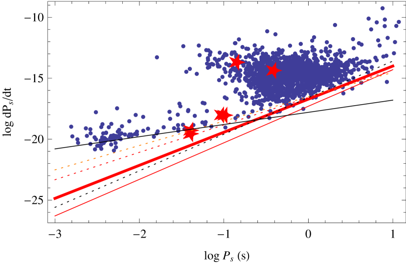
Figure 1.— $P_{\rm s}-\dot{P_{\rm s}}$ diagram superimposed with various death-lines. The stars indicate binaries whose visible lifetime is dominated by the death timescale: all wide PSR-NS binaries (recycled) and PSRs J1141-6545 and J1906+0746 (nonrecycled). The thick solid line is the Chen and Ruderman death-line (Chen & Ruderman, 1993); the thin solid line is from Contopoulos & Spitkovsky (2006); the dotted red lines are from Zhang et al. (2000). The black solid line is the curve ${P_{\rm s}}/{2{\dot{P}}_{\rm s}}=10\rm{Gyr}$; the black dotted line is the curve where ${\dot{E}}=4\pi^{2}I{\dot{P}}{{}_{s}}P{{}_{s}}^{-3}=10^{30}$ erg/s, assuming a moment of inertia I=10⁴⁵ g cm² (Lorimer & Kramer, 2004).

2.3. Beaming Distribution

Except for two pulsars, the empirical beaming geometry of any pulsar in a binary is not tightly constrained. Further, as discussed below, observations of single pulsars suggest that, even restricting to pulsars with similar evolutionary state (e.g., spin), the pulsar beam is randomly aligned relative to its spin axis. Nonetheless, because of the poisson statistics of pulsar detection (KKL), only one property of the intrinsic pulsar geometry distribution matters: the fraction $F(P_{s})[\equiv f_{\rm b,eff}^{-1}]$ of all randomly selected pulsars whose beam crosses our line of sight. Assuming the pulsar beam drops off rapidly – typical models involve gaussian cones – the fraction of all pulsars $F(P_{s})$ of a given spin period and luminosity that emit towards us is well-defined and essentially independent of distance. The main ingredients necessary to calculate $F(P_{s})$ are the half-opening angle $\rho$ of the radio beam and the misalignment angle between pulsar’s spin and magnetic axes $\alpha$. All of our analysis leading to the posterior rate prediction, Eqs. (1) $-$ (3) generalize to an arbitrary beam geometry distribution upon substituting $1/f_{b}\rightarrow F$.

To calculate $F$, for simplicity and following historical convention we assume the bipolar pulsar beam subtends a hard-edged cone with opening angle $\rho$, misaligned by $\alpha<\pi/2$ from the rotation axis. As the pulsar rotates, this beam subtends a solid angle

$$\frac{4\pi}{f_{\rm b}} = {2\pi}\times 2\int_{\rm{min}(0,\alpha-\rho)}^{\rm{max}(\alpha+\rho,\pi/2)}d\cos\theta~{},$$ (7)

where the beaming correction factor $f_{\rm b}$ is the inverse of the fraction of solid angle the beam subtends, given opening and inclination angles ($\rho,\alpha$). This simple model for beam geometry and its correlation with pulsar spin have been explored ever since pulsar polarization data and the rotating vector model made alignment constraints possible, see, e.g., Rankin (1993), Gil & Han (1996), Kramer et al. (1998), Weltevrede & Johnston (2008).In one form or another, this theoretically-motivated semi-empirical correlation has been adopted as an ingredient in most models for synthetic pulsar populations: see, e.g., Arzoumanian et al. (1999a), Gonthier et al. (2004), Gonthier et al. (2006), Faucher-Giguère & Kaspi (2006), Story et al. (2007), and references therein. Conversely, fully self-consistent population models which account for space distribution and kicks, luminosity evolution, beam structure and shape evolution, accretion during binary evolution, and spindown are required, in order to extract all the degenerate parameters that enter into a model by comparing its predictions with observations.

In this paper, we focus on quantifying how much the addition of a spin-dependent opening angle $\rho(P_{\rm s})$ combined with a misalignment angle $\alpha$ distribution influences birthrate estimates. As a simple approximation, we adopt $\alpha$ and $\rho(P_{\rm s})$ distributions that are consistent with the observed pulse widths at 10% intensity level; see Zhang et al. (2003) and Kolonko et al. (2004). Specifically, we assume the misalignment angle is uniformly distributed between [0,$2/\pi$]:

$${\cal P}(\alpha)d\alpha=2/\pi d\alpha~{}.$$ (8)

Other distributions for $\alpha$ have been proposed, from a random vector ${\cal P}(\alpha)=\sin\alpha$ (strongly disfavored by the high frequency with which low-$\alpha$ pulsars have been detected; most detected pulsars would be orthogonal) to more tightly aligned distributions; see for example Fig. 3 in Kolonko et al. (2004). While limited current observations cannot tightly constrain the intrinsic misalignment angle distribution, they strongly suggest tight alignments (low $\alpha$) should be attained at least as often as a flat distribution implies. In Table 3.4 we compare our reference model with several alternative misalignment distributions; only for exceptional misalignment assumptions (e.g., $p(\alpha)\propto 1/\alpha$) will our final results change significantly.

For pulsars with spin period larger than $10{\rm ms}$, we calculate $\rho(P_{\rm s})$ applying a model consistent with classical observations of isolated pulsars’s beam geometry (see,e.g., Weltevrede & Johnston, 2008, and references therein), as shown in Fig. 2

$$\rho(P_{\rm s}) = 5.4^{o}P_{s}^{-0.5}\qquad P_{s}>10~{}{\rm ms}$$ (9a)

The available single-pulsar data does not support a compelling model for rapidly spinning young and recycled pulsars. We adopt an ad-hoc power-law form as our fiducial choice:

$$= 54^{o}(P_{s}/10{\rm ms})\qquad P_{s}<10~{}{\rm ms}$$ (9b)

In both regions, we allow for a small gaussian error in $\ln\rho$ to allow for model uncertainty; we conservatively adopt $\sigma_{\ln\rho}=\ln 1.3$ (i.e., “30%” error; Figure 2 shows a $2\sigma$ interval about our fiducial choice). Based on these two independent distributions, we estimate the fraction of pulsars with spin period $P$ that point towards us as

$$F(P_{\rm s}) \equiv \left<f_{\rm b}^{-1}\right>\equiv 1/f_{\rm b,eff}$$ (10)

The trend of $f_{\rm b,eff}(P_{\rm s})$ shown in Fig. 3 largely agrees with previous estimates of the beaming fraction for nonrecycled pulsars; see, e.g., Tauris & Manchester (1998).

In addition to our fiducial choice, we have explored several other short-period beaming models. As a benchmark for comparison, two extreme cases are provided in Figure 2: a “very narrow” (blue) and “very wide” (green) opening angle model, where the $P^{-1/2}$ truncates at $14^{\circ}$ ($149{\rm ms}$) and $54^{\circ}$ ($10{\rm ms}$), respectively. For relevant spin periods, these extreme alternatives imply noticeably different amounts of beaming correction from each other and our fiducial model, up to $O(\times 2)$; see Figure 3. Nonetheless, our best semi-empirical estimates for binary pulsar birthrates are fairly or highly insensitive to the precise opening angle model $\rho(P)$ adopted for rapidly spinning pulsars. As described below, for pulsars with $10{\rm ms}<P_{s}<100{\rm ms}$, we anchor our theoretical bias with observed geometries of comparable binary pulsars. In this period interval, the choice for $\rho(P)$ effectively serves as an upper bound on plausible $\rho$ (and sets a lower bound on $f_{\rm b}$).

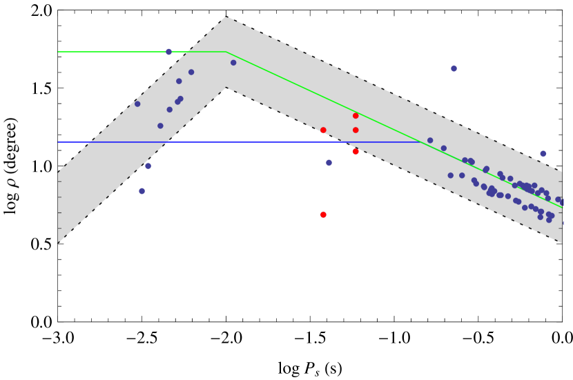
Figure 2.— Opening angles $\rho(P_{\rm s})$ versus spin period for a sample of pulsars drawn from Kramer et al. (1998) and PSRs B1913+16 (Weisberg & Taylor, 2002) and B1534+12 (Arzoumanian et al., 1996). For pulsar binaries where multiple conflicting measurements of $\rho$ exist, all values are shown (red points). For pulsars with P${}_{\rm s}<$ 10 ms or P${}_{\rm s}>$ 100 ms, we adopt an empirically-motivated relation for $\rho(P_{s})$, including $\rho\propto$ P${}_{\rm s}^{-0.5}$ at large $P$; this distribution, allowing for scatter (the shaded region) is used to calculate the effective beaming correction factor $f_{\rm b,eff}$ over many pulsars with a similar spin; see Eq. 10. For pulsars with spin period 10 ms $<$ P_s $<$ 100 ms, we define an alternative ‘conservative’ beaming model such that $f_{b}=6$ (not shown). In this interval, to reflect our uncertainty in pulsar opening angle models, we assume $\ln f_{\rm b}$ is uniformly distributed between the ‘standard’ beaming model implied by this figure’s $\rho(P)$ and the ‘conservative’ choice $f_{b}=6$. Finally, the thin and dashed lines indicate two extreme alternative opening angle models discussed in §2.3.

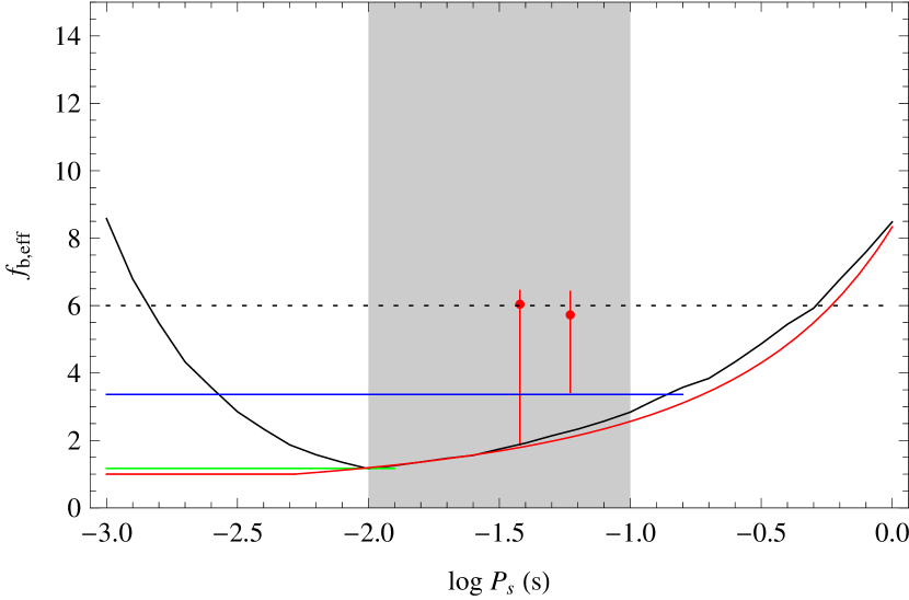
Figure 3.— The effective beaming correction factor $f_{\rm b,eff}$ versus pulsar spin period $P_{s}$ (black), assuming the distribution of beaming geometries described in the text. For comparison, we show comparable estimates for the beaming correction factor from Tauris & Manchester (1998) as a red curve (using their Eq. 15, but extended beyond the $P=0.1-5~{}{\rm s}$ region they fit) as well as the observed $P_{s}-f_{\rm b}$ combinations for PSRs B1913+16 (log P${}_{\rm s}=-1.23$) and B1534+12 (log P${}_{\rm s}=-1.42$), based on the preferred values adopted in Kalogera et al. (2001) (red points) and all possible combinations of values for $\alpha$ and $\rho$ provided in Arzoumanian et al. (1996), Kramer et al. (1998) ( red vertical bar). Finally, the gray shaded region indicates the spin period interval (10 ms $<P_{s}<$ 100 ms), where few pulsar opening angles are available to constrain our model; see Kramer et al. (1998). Also shown in green and blue are the effective beaming factors implied for the extreme “narrow” and “wide” models shown in Fig. 2.

Any specific choice of opening angle and misalignment distribution ${\cal P}(\alpha,\rho|P_{\rm s})$ determines that model’s probability ${\cal P}(f_{b}|P_{\rm s})$ that a randomly selected pulsar with spin period $P_{\rm s}$ has beaming correction factor $f_{b}$

$${\cal P}(f_{b}|P_{\rm s})df_{b} = \int\delta(f_{b}-f_{b}(\alpha,\rho)){\cal P}(\rho|P_{\rm s})d\rho{\cal P}(\alpha)d\alpha$$ (11)

Further, because $1/f_{b}$ is the probability that a given randomly selected pulsar points towards us, the distribution $p_{e}$ of $f_{b}$ among the fraction $F$ of all pulsars aligned with our line of sight is

$${\cal P}_{e}(f_{b}|P_{\rm s})df_{b} = \frac{{\cal P}(f_{b}|P_{\rm s})/f_{b}}{F(P_{\rm s})}$$ (12)

For our fiducial beaming model, Fig. 4 compares the median value of $f_{b}$ for the two distributions as a function of $\rho(P_{\rm s})$. It shows the beaming correction factors $f_{b}$ for the detected population of pulsars can differ substantially from the underlying population, if only because those pulsars with narrow beam coverage (i.e., $f_{b}\gg 1$) are less likely to be detected. Only extremely narrow pulsar beams $\rho<10^{o}$ will lead to a typical detected pulsar with $f_{b}\simeq 6$, comparable to the measured value for known PSR-NS binaries that was adopted in previous analyses as the canonical value; see Fig. 3.

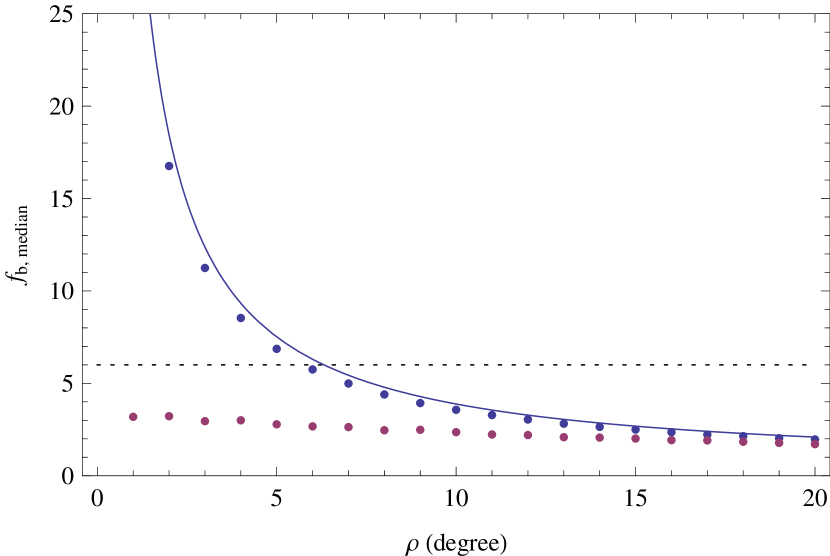
Figure 4.— The median value of $f_{\rm b}$ for detectable pulsars (red; from ${\cal P}_{e}$ in Eq. (12)) and all pulsars (blue; from ${\cal P}$ in Eq. (11)) versus $\rho$, assuming a synthetic pulsar population with misalignment angle $\alpha$ uniformly distributed and beaming described by Eq. (7). Also shown is $1/f_{\rm b}=(1-\cos\rho)+(\pi/2-\rho)\sin\rho$, an estimate of $f_{\rm b}(\rho)$ assuming $\alpha$ is random; see Emmerling and Chevalier (1989). The detectable pulsar population will preferentially have wide beams. Only a population of pulsars with very tight opening angles are consistent with the canonical value of $f_{\rm b}=6$. In our “standard” model (Eqs. 7 and 8), such narrow beams are improbable for pulsars spinning with $10{\rm ms}<P_{s}<100{\rm ms}$ that is relevant to most of the known PSR-NS binaries (see Table 1).

2.4. Partial information and competing proposals

In a few cases, observations ${\cal O}_{i}$ of pulsar $i$ provide some information about that pulsar’s geometry, such as confidence intervals on $\alpha$ and $\rho$ or even a posterior distribution function ${\cal P}(\alpha,\rho|{\cal O}_{i})$. When a unique, superior constraint exists, we could have simply factored this information into the average that defines $F=1/f_{\rm b,eff}$ (Eq. 9) (e.g., $\alpha$ constraints for PSR J1141-6545; the preferred geometries of PSRs B1913+16 and B1534+12). However, in cases where competing proposals exist (e.g., the two models for PSR J0737-3039A suggested by Demorest et al. (2004) and Ferdman et al. (2008), also reviewed in Kramer & Stairs (2008); see §3.1), or where our prediction is extremely sensitive to unavailable priors, such as the mean misalignment angle of PSR J1141-6545, (Manchester et al., 2010; Kramer, 2008) (§3.3), we explicitly provide multiple solutions in the text. When multiple competing predictions are available, our final prediction averages over a range of predictions between them. Explicitly, if ${\cal P}_{f}(\log f_{\rm b})$ is a distribution in $X\equiv\log(f_{\rm b}/f_{\rm b,eff})$ reflecting our a priori model uncertainty in $f_{\rm b,eff}$, and ${\cal P}(\log{\cal R}|f_{\rm b})={\cal R}{\cal P}({\cal R}|f_{\rm b})\ln 10$ is our posterior estimate for the birthrate ${\cal R}$ given known beaming $f_{\rm b}$ [cf. Eq. 1], then a posterior estimate that reflects uncertain beaming is

$${\cal P}(\log{\cal R})d\log{\cal R} = \int dX{\cal P}_{f}(X+\log f_{\rm b,eff}){\cal P}(\log{\cal R}-X|f_{\rm b,eff})~{}.$$ (13)

For the many PSR-NS binaries which have spin period between 10 ms and 100 ms,we calculate P(log R) using Eq. (11). Specifically, we average P(log R) over the beaming correction factor between $f_{\rm b,eff}$ (listed in Table 1) and the canonical value of 6, adopting a systematic error distribution $P_{sys}$(log $f_{\rm b}$) which is uniform in log $f_{\rm b}$ between these limits. For pulsars with spin period outside of this range, we use Eq. (1) with $f_{\rm b,eff}$ listed in Table 1 or 2.

Table 1Properties of PSR-NS binaries considered in this work. For most pulsars, $f_{b,eff}$ averages over the half-opening angle $\rho$ and misalignment angle $\alpha$. For PSR J0737-3039B, we adopt the preferred choice for $\alpha\simeq 90^{o}$ and average only over the stated uncertainties in $\rho$(P_s). For PSRs B1913+16 and B1534+12, where both $\alpha,\rho$ measurements are available, we adopt the values of $f_{b,obs}$ from Kalogera et al. (2001). The final column is $C=\tau_{i}/N_{psr}f_{b}$, also see, Eq. (1) and Eq. (4). When numbers are uncertain, this table shows self-consistent fiducial choices. Significant uncertainties are included by explicit convolutions described in the text. Small uncertainties are ignored; for example, our Monte Carlo estimates for $N_{psr}$ have poisson sample-size errors of roughly $1/\sqrt{N_{det}}\simeq O(2-5\%)$, where $N_{det}=10^{6}/N_{psr}$.

PSR Name	$P_{\rm s}$	$\dot{P_{\rm s}}$	$M_{\rm psr}$	$M_{\rm c}$	$P_{\rm orb}$	e	$f_{\rm{b,obs}}$	$f_{\rm{b,eff}}$	$\tau_{\rm age}^{a}$	$\tau_{\rm mgr}$	$\tau_{\rm d}$	$N_{\rm psr}$	$C$	Refb
	(ms)	$10^{-18}$ (ss-1)	($M_{\odot}$)	($M_{\odot}$)	(hr)				(Gyr)	(Gyr)	(Gyr)		(kyr)
tight binaries
B1913+16	59.	8.63	1.44	1.39	7.75	0.617	5.72	2.26	0.0653	0.301	4.31	576	111	1,2
B1534+12	37.9	2.43	1.33	1.35	10.1	0.274	6.04	1.89	0.200	2.73	9.48	429	1130	3,4
J0737-3039A	22.7	1.74	1.34	1.25	2.45	0.088		1.55	0.142	0.086	14.2	1403	105	5
J0737-3039B	2770.	892.			2.45	0.088		14.	0.0493		0.039			6
J1756-2251	28.5	1.02	1.4	1.18	7.67	0.181		1.68	0.382	1.65	16.1	664	1821	7
J1906+0746	144.	20300.	1.25	1.37	3.98	0.085		3.37	0.000112	0.308	0.082	192	126	8,9
wide binaries
J1518+4904	40.94	0.028	1.56	1.05	206.4	0.249		1.94	29.2	$>\tau_{H}$	51.0	276	18,700	10, 11
J1811-1736	104.18	0.901	1.60	1.00	451.2	0.828		2.92	1.75	$>\tau_{H}$	7.9	584	5860	12,13
J1829+2456	41.01	0.053	1.14	1.36	28.3	0.139		1.94	12.3	$>\tau_{H}$	43.0	271	19,000	14
J1753-2240c	95.14	0.97	1.25	1.25	327.3	0.303		2.80	1.4	$>\tau_{H}$	8.2	270	13,900	15

Figure 5.— Solid curve: our estimate for the birthrate of pulsars like PSR J0737-3039A, based on our standard beaming geometry model ($f_{\rm b,eff}=1.55$) and its spindown age ($\tau_{age}=145{\rm Myr}$). Dotted curve: as previously, but marginalized over uncertainties in the age $\tau_{age}$. Motivated by averaging together models 1,4, and 5 in Lorimer et al. (2007), assuming each model equally likely, we approximate age uncertainty in PSR J0737-3039A by a uniform distribution in $t$ between 50 and 180 ${\rm Myr}$. While significantly shorter lifetimes are permitted, the median birthrate for pulsars like PSR J0737-3039A increases by only $20\%$, from 18${\rm Myr}^{-1}$to 22 ${\rm Myr}^{-1}$.

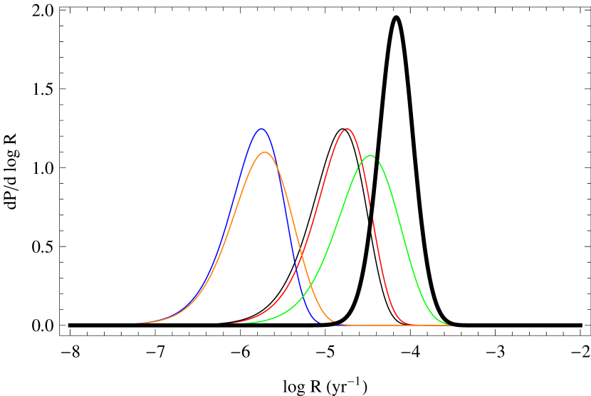
Figure 6.— Distributions ${\cal P}(\log{\cal R})$ for the birthrate of tight PSR-NS binaries: PSRs B1913+16 (red), B1534+12 (blue), J0737-3039A (green), J1756-2251 (orange), and J1906+0746 (black). The thick black curve indicates our best estimate for the overall Galactic birthrate of tight PSR-NS binaries, assuming the reference pulsar population model in KKL06; the median value is $\simeq 89~{}{\rm Myr}^{-1}$. The individual colored curves indicate our best estimates for the birthrate of the individual binaries, based on Eq. (1) and incorporating $f_{\rm b,eff}$ listed in Table 1. For the two PSRs with $10~{}{\rm ms}<P_{\rm s}<100~{}{\rm ms}$ and without specified beam geometry (PSRs J0737A-3039 and J1756-2251), we account for uncertainty in opening-angle modeling by allowing $\ln f_{\rm b}$ to be anywhere between our ‘conservative’ and ‘standard’ choices.

Table 2 Properties of tight PSR-WD binaries considered in this work. For all binaries here, $f_{\rm{b,eff}}$ averages over the half-opening angle $\rho$ and misalignment angle $\alpha$.Monte Carlo sampling uncertainty in $N_{psr}$ is roughly $1/\sqrt{N_{det}}\simeq O(3-5\%)$

PSR Name	$P_{\rm s}$	$\dot{P_{\rm s}}$	$M_{\rm psr}$	$M_{\rm c}$	$P_{\rm orb}$	e	$f_{\rm{b,eff}}$	$\tau_{\rm age}^{a}$	$\tau_{\rm mgr}$	$\tau_{\rm d}$	$N_{\rm psr}$	$C$	Refb
	(ms)	$10^{-18}$ (ss-1)	($M_{\odot}$)	($M_{\odot}$)	(hr)			(Gyr)	(Gyr)	(Gyr)		(kyr)
J0751+1807	3.48	0.00779	1.26	0.12	6.32	$<10^{-7}$	2.62	6.66	9.48	$>\tau_{H}$	2404	1588	1,2
J1757-5322	8.87	0.0278	1.35	0.67	10.9	$<10^{-6}$	1.26	7.16	8.0	145	1082	7335	3
J1141-6545	393.9	4295.	1.3	0.986	4.74	0.172	5.46	0.00145	0.60	0.10	346	53	4,5
J1738+0333	5.85	0.0241	1.7	0.2	8.5	$4\times 10^{-6}$	1.69	3.71	10.8	$>\tau_{H}$	609	9716	6

Similarly, if the lifetime is uncertain, one can marginalize $P(\log{\cal R})$ over the lifetime $\tau$; if the relative likelihood of different lifetimes ${\cal P}_{\tau}(\log\tau_{i})$ is known, then defining $Y=\log({\tau}/\tau_{i})$,

$${\cal P}(\log{\cal R})d\log{\cal R} = \int dY{\cal P}_{\tau}(Y+\log\tau_{i}){\cal P}(\log{\cal R}+Y|\tau_{i})~{},$$ (14)

Though usually the lifetime is relatively well determined, being dominated by relatively well determined merger or death timescale, we do use this expression to marginalize over the considerable uncertainty in the current age of PSR J0737-3039A, based on the proposed range of lifetimes presented by Lorimer et al. (2007); see Fig. 5.

3. RESULTS

3.1. Tight PSR-NS binaries

The pulsar binaries we consider in this work and the estimated $f_{\rm b,eff}$ based on our standard model are summarized in Table 1 and 2. Tight PSR-NS binaries contribute to our estimate of the overall PSR-NS birthrate (which, for these short-lived systems, is equivalent to their merger rate). Among this set, both PSRs B1913+16 and B1534+12 have both $\rho$ and $\alpha$ measurements. For PSR B1913+16, we adopt $f_{b,obs}=5.72$ based on $\rho=12.4^{\circ}$(Weisberg & Taylor, 2002) and $\alpha=156^{o}$. For PSR B1534+12, we use $f_{b,obs}=6.04$ based on $\rho=4.87^{\circ}$ and $\alpha=114^{o}$ (Arzoumanian et al., 1996). [The canonical value of $f_{\rm b}\sim 6$ is obtained from the average of the $f_{b,obs}$ for these pulsars.] Alternative choices for $\alpha$ and $\rho$ have been proposed for both pulsars (Fig. 3); combining the most extreme of these options leads to values comparable to our model’s preferred values: $f_{\rm b,eff}=$ 2.2 and 1.8 for PSRs B1913+16 and B1534+12 respectively. As tightly beamed pulsars are unlikely to be seen in our fiducial or tightly beamed model [the solid and dashed curves in Fig. 3], we adopt an alternative approach for pulsars with spin periods in the otherwise poorly constrained region $10$ and $100{\rm ms}$, the interval containing most PSR-NS binaries.

Pulsars in tight PSR-NS binaries may have wide opening angles, given their spin periods (see Fig. 2). If so, these binaries likely have $f_{\rm b}<6$. However, the observations suggest that PSRs B1913+16 and B1534+12 have narrower beams (see Fig. 2, region defined by dotted lines). If these narrower opening angles are characteristic of tight, recycled pulsars in PSR-NS binaries, the appropriate $f_{\rm b}$ could be closer to $6$. In particular, given the similarity in spin period of PSR J0737-3039A to those pulsars and the lack of other constraints in that period interval (see Fig. 2), we assume $\log f_{\rm b}$ could take on any value between $\log 1.5$ (the value we estimate in our spin model) and $\log 6$.

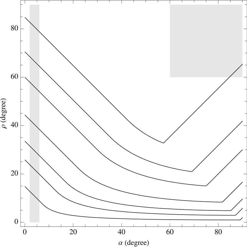
Figure 7.— Plausible beaming in PSR J0737-3039A: Solid curves are contours $f_{\rm b}(\alpha,\rho)$ corresponding to $f_{\rm b}=1.1,1.5,2,3.5,6,10,30$ (top to bottom). Overlaid are approximately-drawn regions of $\alpha$ and $\rho$ which are consistent with observations of PSR J0737-3039A, corresponding to the unipolar model (left box, small $\alpha$) and two-pole model (right box); compare with contours and discussion in Demorest et al. (2004).

Given posterior likelihoods, we could explicitly and systematically include observational constraints on the beaming geometry of PSR J0737-3039A as described earlier; see, e.g., the posterior constraints in Demorest et al. (2004) and Ferdman et al. (2008). Observations support two alternate scenarios. In one, the pulse is interpreted as from a single highly aligned pole ($\alpha<4^{\circ}$). Because of its tight alignment, in this model the beaming correction factor should be large: at least as large as those for binary pulsars ($f_{b}\simeq 6$, assuming $\rho\sim 30^{\circ}$, from $\rho(P_{\rm s})$), and potentially larger ($f_{b}\simeq 30$ assuming $\rho=10^{\circ}$, based on observed opening angles for PSRs B1913+16 and B1534+12). In the other scenario, favored by recent observations (Ferdman et al., 2008), the pulse profile is interpreted as a double pole orthogonal rotator $\alpha\simeq\pi/2$ with a fairly wide beam ($\rho\sim$60${}^{\circ}-$90^∘, consistent with $\rho(P_{\rm s})$). This latter case is consistent with our canonical model and leads to a comparable $f_{b}$. Comparing with the assumptions presented earlier, so long as we ignore the possibility of tight alignment and narrow beams, our prefered model and uncertainties for PSR J0737-3039A already roughly incorporate its most significant modeling uncertainties. Considering that the contribution from PSR J1906+0746 is comparable with that of the PSR J0737-3039A, our best estimate for the birthrate of merging PSR-NS binaries is not very sensitive to changes in a nearly orthogonal-rotator geometry model for PSR J0737-3039A. However, because we cannot rule out the most extreme scenarios for PSR J0737-3039A, for completeness we also describe implications of a unipolar model: the beam shape constraints summarized by Fig. 7 translate to a prior on $\log f_{b}$ that is roughly uniform between $\log 6$ and $\log 30$.

In Fig. 6, we show that the probability distribution of PSR-NS merger rate with our best estimates for the beaming correction $f_{\rm b,eff}$, assuming the reference model of KKL06. $P({\cal R}$)’s follow from convolving together birthrate distributions based on each individual pulsar binary, where those birthrate distributions are calculated as described in previous sections. Including PSR J1906+0746, we found the median PSR-NS merger rate is $\simeq 89$ Myr^-1, which is smaller than what we predicted in KKL06 ( $\sim 123$ Myr^-1, cf. their peak value is 118 Myr^-1), assuming the same $\tau_{age}$ and $\tau_{mrg}$ listed in Table 2, but used $f_{b,J0737}=5.9$, due entirely to the smaller beaming correction factors for PSR J0737-3039A allowed for in this work. Though our best estimate for the merger rate is slightly smaller than previous analyses, the difference is comparable to the Poisson-limited birthrate uncertainty and much smaller than the luminosity model uncertainty described in the appendix. Being nearly unchanged, our study has astrophysical implications in agreement with prior work such as PSCand O’Shaughnessy et al. (2009).

Although the merging timescale is reletively well-defined, we note that our estimate does not include $O(30\%)$ uncertainties in the current binary age. In this work, for example, we fix the total age of PSR J0737-3039A to be $\sim$230 Myr. Fig.  5 shows a marginalized P(${\cal R}$) using the age constraints from (Lorimer et al., 2007) between 50 and 180 ${\rm Myr}$ (These models take into account interaction between the two pulsars; we omit the two most extreme models 2 and 3 with rapid magnetic field decay).

3.2. Wide PSR-NS binaries

In addition to those in tight orbits, some PSR-NS binaries have wide orbits (orbital period is larger than 10 hours). These wide binaries would never merge through gravitational radiation within a Hubble time. Their estimated death timescales imply that most of the known pulsars in wide binaries will remain visible for time comparable to or in excess of $10~{}{\rm Gyr}$ (see Table 1) and that binaries have accumulated over the Milky Way to their present number. In this work, we assume that PSR J1753-2240 (Keith et al., 2009) is another wide PSR-NS binary. Motivated by the fact that spin periods of pulsars found in wide orbits are comparable to those relevant to tight PSR-NS binaries, we adopt the same techniques for estimating $f_{\rm b,eff}$. For PSRs J1811-1736 and J1753-2240, we adopt the $f_{\rm b,eff}$ values expected from their spin periods. On the other hand, for PSRs J1518+4904 and J1829+2456, we average ${\cal P}({\cal R}|f_{\rm b})$ over a range of $\ln f_{\rm b}$ between the value predicted ($\ln f_{\rm b,eff}$ listed in Table 1) and $\ln 6$. Our estimate for the birthrate of “wide” PSR-NS binaries, shown in Fig. 8, is slightly higher than previously published estimates by PSC. The birthrate of wide PSR-NS binaries is not significantly changed due to the discovery of PSR J1753-2240, because of its resemblance to PSR J1811-1736. Contrary to § 2, the previous analyses had assumed that the pulsar population reached number equilibrium, e.g., O’Shaughnessy et al. (2005); our effective lifetime is 2 times shorter. At the same time, our beaming correction is roughly three times smaller, so the relevant factors mostly cancel; our median prediction is almost exactly 1.5 times lower than the previous estimate.

The reconstructed $P({\cal R}$) assuming steady-state star formation has a median at 0.84 Myr^-1 and is narrower than the previous work due to the discovery of PSR J1753-2240, with a ratio between the upper and lower rate estimate at 95% confidence interval, ${\cal R}_{95\%}/{\cal R}_{5\%}$, is 8.8 (compared to 13.8 without J1753-2240). As in PSC, the birthrate estimate of “tight” PSR-NS binaries is still roughly 100 times greater than that of “wide” binaries, even though both estimates have been modified through lifetime and $f_{\rm b,eff}$ corrections. Interestingly, known “wide” PSR-NS binaries were discovered through recycled pulsars exclusively. Following PSC, we interpret the difference in birthrate as evidence for a selection bias: only a few progenitors of PSR-NS binaries undergo enough mass transfer to spin up the PSR, but not enough to bring the orbit close enough to merge.

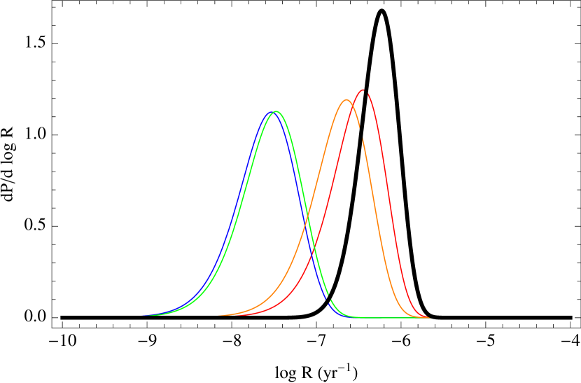
Figure 8.— Same as Fig. 6, but for the wide PSR-NS population: PSRs J1811-1736 (red), J1518+4904 (blue), J1829+2456 (green), and J1753-2240 (orange), along with our best guess for the overall rate (thick black curve). The median birthrate for wide PSR-NS binaries is $0.84~{}{\rm Myr}^{-1}$, assuming the preferred pulsar population model in KKL06 and a steady star formation rate. The newly discovered PSR J1753-2240 is a cousin of PSR J1811-1736: their contributions to the Galactic birthrate are comparable.

3.3. Tight PSR-WD binaries

With the exception of PSR J1141-6545, the lifetimes of tight PSR-WD binaries are limited by their gravitational wave inspiral time (Peters, 1964). The net visible lifetimes of these binaries are significantly in excess of the age of the Milky Way, and are strongly recycled with $P<10~{}{\rm ms}$. Based on comparison with measured isolated pulsars, a likely range for their opening angles and thus $f_{\rm b,eff}$ can be estimated (see Table 2 for a summary). Combining this information, birthrates for the three millisecond PSR-WD binaries, PSRs J0751+1807, J1757-5322, and the newly discovered J1738+0333, are easily estimated (Fig. 10). The birthrate for tight PSR-WD binaries, however, is dominated by the non-recycled pulsar PSR J1141-6545. For this unusual binary, the visible pulsar lifetime is dictated by its death timescale ($\tau_{\rm d}$), rather than its gravitational-wave merger time ($\tau_{\rm mrg}$), e.g., Kim et al. (2004). Based on different models for the death line, we expect the total lifetime of PSR J1141-6545 to be between between $100-170$ Myr; for the purposes of a rate estimate, we allow $\tau$ to be logarithmically distributed within these limits. Additionally, recent observations imply its misalignment angle to be $160^{\circ}$${}^{+8}_{-16}$ (or equivalently, $12^{\circ}<\alpha<36^{\circ}$, which is adapted in this work) at a 68% confidence level, (Manchester et al., 2010; Kramer, 2008); see Fig. 9. Without this alignment information we would already predict fairly substantial beaming: $f_{\rm b,eff}\approx 5.46$ solely based on $\rho(P_{\rm s})\approx 8{{}^{\circ}}.6$ (Table 2). With a nearly-polar beam, however, the beaming could be $10$ times tighter. We therefore present two estimates for the birthrate of PSR J1141-6545, contingent on $\alpha$: our current a priori model, shown as a solid curve in Fig. 9; and an estimate that includes tight beaming (dotted curve).

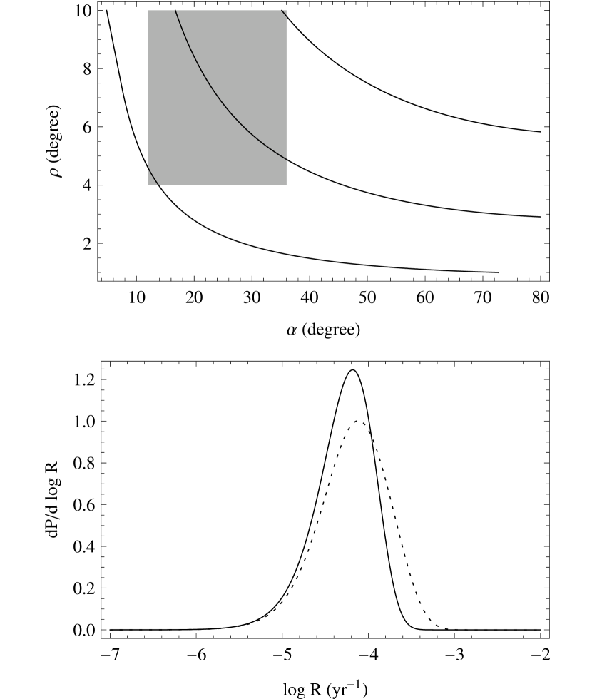
Figure 9.— Top panel: A contour plot of $f_{b}(\alpha,\rho)$ over the range relevant to PSR J1141-6545; contours shown are $f_{b}=5,10,30$ from top to bottom, respectively. The shaded region indicates the range of $\alpha$ and $\rho$ implied by a preliminary analysis of recent observations Manchester et al. (2010); Kramer (2008); inside this box $f_{\rm b}$ ranges between 5 and 30. Bottom panel: ${\cal P}({\cal R})$ for PSR J1141-6545 based on our standard model ($f_{\rm b,eff}=$ 5.46; solid, also see Table 2) and the constraints above (averaging $f_{\rm b,eff}$ between 5.46 and 30 using Eq. (13); dashed).

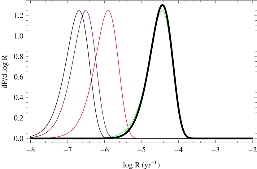
Figure 10.— Empirical distributions ${\cal P}(\log{\cal R})$ implied by the set of known, tight PSR-WD binaries: PSRs J1141-6545 (green), J1757-5322 (purple), J0751+1807 (red), and J1738+0333 (blue), given the assumptions about opening angle and misalignment. The P(${\cal R}$) for PSR J1141-6545 presented here (solid green curve) is obtained by our standard prediction: assuming the pulsar is one of a family of pulsars with misalignment angles $\alpha$ uniformly distributed between $0$ and $\pi$ and $\rho$ normally distributed as in Fig. 2 (cf. see Fig. 9). Based on our standard beaming geometry model, PSR J1141-6545 still dominates the Galactic birthrate of PSR-WD binaries. The median rate for the Galactic PSR-WD binaries (thick black solid curve) is estimated to be $\simeq 34~{}{\rm Myr}^{-1}$

Pulse profiles are an essential ingredient in empirical pulsar population modeling. The pulse profile of PSR J1141-6545 has significantly broadened, by a factor 8, since the pulsar was discovered in 2000 (Kramer, 2008). This is mainly attributed to the effects of the geodetic precession. Recalculating $N_{psr}$ for PSR J1141-6545 with the current, broader pulse, the most likely value of $N_{psr}$ is now $\sim$1000 instead of 350 that is estimated with the pulse profile in 2000 (see Kim et al. (2004) for the details). We expect that an analysis that treats both geodetic precession and the duration of pulsar radio surveys imply a slightly different birthrate for the PSR J1141-6545 than what has been shown in Kim et al. (2004). In this work, however, we use the pulse profile presented in the discovery paper (Kaspi et al., 2000) and assume no evolution in the pulse probile, as we only focus on the effects of the beaming correction factor with various beam geometry models. The effects of the pulse profile evolution of PSR J1141-6545 to the Galactic birthrate of PSR-WD binaries, taking into account more detailed corrections for observational biases such as the Doppler smearing, will be discussed in a separate paper (Kim et al. in prep).

Our preferred birthrate estimate agrees with previously published estimates based on a “fidicual” beaming factor $f_{\rm b}=6$ [PSC; compare $C=53{\rm kyr}$ here with $A=47{\rm kyr}$ in their Table 1 for PSR J1141-6545], as well as with early estimates that adopt $f_{\rm b}=1$ [Kim et al. (2004) predict a peak-probability galactic birthrate of $4f_{b}$${\rm Myr}^{-1}$, based on an $N_{psr}=400$]. By coincidence the fiducial beaming factor agrees with our best beaming estimates based on $\rho(P)$ data for comparable-spin pulsars. Our birthrate estimate also agrees with a recently published independent estimate of PSR-NS (or PSR-BH) birthrates based on optical discovery of the tight WD-compact object binary SESS 1257+5428 described in Thompson et al. (2009).

3.4. Discussion

Table 3Comparison of effective beaming correction factors $f_{\rm b,eff}$ predicted by different pulsar geometry models (columns 3–6): flat ($p(\alpha)=2/\pi$ ; adopted in the text, see Eq. 8); $p(\alpha)=\cos\alpha$; $p(\alpha)$ as proposed by Eq. (12) of Zhang et al. (2003) (ZJM03); and $p(\alpha)\propto 1/\alpha$ between $3^{\circ}$ and $90^{\circ}$. Reading from left to right, misalignment models correspond to an increasing fraction of fairly aligned pulsars; for example, the last distribution has half of all binaries with $\alpha<16^{\circ}$, which for the pulsars of interest usually corresponds to $f_{\rm b}>10$. Nonetheless, the relevant effective beaming correction factor does not increase as rapidly as the largest (or even median) $f_{\rm b}$. Generally, when $p(\alpha)$ has a subpopulation of tightly-aligned pulsars, $f_{\rm b,eff}$ is inversely proportional to the fraction of binaries with large misalignments, as well as being directly proportional to the median $f_{\rm b}$ for the large-misalignment subpopulation. Therefore, large $f_{\rm b,eff}$ values are only possible if a significant fraction of pulsars are assumed to be tightly aligned; such a hypothesis is difficult to test, as these tightly aligned pulsars will be extremely difficult to see.

Name	$f_{b,obs}$	flat	ZJM03	$\cos\alpha$	$1/\alpha$
tight PSR-NS
B1913+16	5.72	2.26	2.63	2.62	3.37
B1534+12	6.04	1.89	2.14	2.13	2.69
J0737-3039A		1.55	1.70	1.69	2.08
J1756-2251		1.68	1.88	1.87	2.33
J1906+0746		3.37	4.05	3.98	5.25
wide PSR-NS
J1518+4904		1.94	2.21	2.21	2.81
J1811-1736		2.92	3.46	3.42	4.48
J1829+2456		1.94	2.22	2.21	2.79
J1753-2240		2.8	3.3	3.27	4.28
tight PSR-WD
J0751+1807		2.62	3.08	3.06	4.00
J1757-5322		1.26	1.35	1.33	1.57
J1141-6545		5.46	6.66	6.46	8.65
J1738+0333		1.69	1.90	1.89

Alternate misalignment models: In order to calculate $f_{\rm b,eff}$, we adopt a flat distribution as our standard model for the $\alpha$ distribution defined in Eq. (8). Several alternative distributions for pulsar misalignment have been proposed; some, however, do not self-consistently account for detection bias. For example, a randomly aligned beam vector on the sphere ($p(\alpha)d\alpha=d\cos\alpha$) implies that nearly all detected pulsars should be nearly orthogonal rotators. The observation of many pulsars with smaller $\alpha$, e.g., Kolonko et al. (2004), is not consistent with that distribution. On the other hand, a flat distribution and even more centrally concentrated ones (e.g., $p(\alpha)=\cos\alpha d\alpha$) are plausible, considering observational biases can explain the lack of detected pulsars with small $\alpha$ (say, $<$ 45^o from Fig. $3$ in Kolonko et al. (2004)). But because the expectation defining $f_{\rm b,eff}$ (Eq. 9) is governed by the smallest typical beaming fraction of detected pulsars, the predictions for $f_{\rm b,eff}$ are fairly independent of misalignment model, assuming it is not too concentrated near the equator or poles. For this reason, and without more information to quantify uncertainties in a reconstructed $\alpha$ distribution with which to base a comparison (e.g., the selection bias of having an $\alpha$ measurement), we choose a flat distribution for simplicity.

What beaming to use?: No one beaming correction factor applies for all circumstances: even for a fixed beam geometry distribution, different “natural” choices $f_{\rm b}$ make sense for different questions [Figure 4]. Beaming depends strongly on spin. Finally, the canonical choice $f_{\rm b}=6$ implicitly requires exceptionally tight beaming, strong alignment, or both [Figure 4 and Table 3.4]. If one number must be adopted, use the spin-dependent relation proposed by Tauris & Manchester (1998) for pulsars with $P>100{\rm ms}$ [Figure 3].

4. Conclusions

In this paper, we revise estimates for the birthrate of Galactic pulsar binaries, including new binaries as well as updated binary parameters and uncertainties. We describe a new quantity, the “effective beaming correction factor” $f_{\rm b,eff}$, as a tool to permit reconstruction of Galactic binary pulsar birthrates from observations, when observations support not just one choice but a distributions of pulsar beam geometries. Currently, the best constrained $f_{\rm b}$’s are available for PSRs B1913+16 and B1534+12, $f_{b,obs}\sim 6$. Previous empirical birthrate estimates like KKL06 adopted this factor for all pulsar binaries, ignoring experience from isolated pulsars’ beams. Instead, we adopt random misalignment angles and a fiducial choice for $\rho(P_{\rm s})$. As summarized in Tables I and II, this choice produces $f_{\rm b,eff}$ significantly smaller than the canonical value of 6 for most pulsar binaries (cf. also see Table 3.4 for comparisons between differerent beam geometry models), and for $P_{\rm s}>10{\rm ms}$ in agreement with the simple expression provided by Tauris & Manchester (1998). Generally, a detected pulsar should be a priori assumed to have nearly as large a beam (as small an $f_{\rm b}$) as its spin allows. Although possible, tight beams cross our line of sight rarely. Unless implicitly assumed ubiqutous, tightly beamed pulsars will not significantly impact a birthrate estimate. For pulsars with spin period between 10 ms and 100 ms, where few observations exist to justify extrapolations, we anchor our theoretical expectations for wide beams with observations of comparable pulsar binaries that suggest strong beaming, averaging between the two extremes. Most of the pulsar binaries that dominate $P({\cal R})$ have spin periods in intervals where $\rho(P_{\rm s})$ is well-sampled. Of the three classes of binaries considered, only the birthrate of wide PSR-NS binaries is dominated by pulsars in the least-well-constrained interval $P_{\rm s}$ between $10$ and 100 ms. Finally, the two binaries PSRs J1141-6545 and J0737-3039A that dominate the birthrate of tight PSR-WD and PSR-NS binaries, respectively, have constrained beam geometries. In both cases, the plausible beam geometries allow a significantly narrower beam and thus a correspondingly higher birthrate. For these two pulsars and more generally for any pulsar binary with spin periods between $10$ and $100$ ms, empirical posterior distributions ${\cal P}(\rho,\alpha)$, if made available, would help us better determine model-independent detected beam geometries and therefore improve our estimates of pulsar binary birthrates.

Studies of nonrecycled pulsars (most with $P\simeq O(0.1-2~{}{\rm s})$) have suggested that isolated and binary pulsars could align their spin and magnetic axes ($\alpha\rightarrow 0$) on $O(70,200~{}{\rm Myr})$ timescales respectively (Weltevrede & Johnston, 2008). While spin-beam alignment leads to narrower beams and therefore significantly increased typical $f_{\rm b}$ for older nonrecycled pulsars, almost all the pulsars studied here are recycled; the two nonrecycled PSRs J1906+0746 and J1141-6545 are far too young for the proposed process to occur. At the other extreme, Young et al. (2009) recently proposed extremely rapid alignment for isolated pulsars, where on short alignment timescales $\simeq 1{\rm Myr}$ beams align and the opening angles converge to $\rho_{\infty}\approx 2-5^{o}$. If applied to the typical $\tau_{i}\simeq O(100{\rm Myr})$ binary pulsars considered here, this model implies exceptionally strong beaming ($f_{\rm b}\simeq 2/\rho_{\infty}^{2}\simeq O(200)$) and, for example, merging PSR-NS birthrates comparable to the galactic supernova rate. In a forthcoming paper we will address time-dependent effects like alignment in pulsar binaries. At present, our birthrate estimate relies only on observed pulsars as representatives of their evolutionary classes, without any correction for when along their evolutionary track they have been detected (e.g., in luminosity or, here, beam size; cf. Phinney & Blandford (1981)).

We find similar binary pulsar birthrates as previous studies when we adopt the same reference pulsar population model as KKL06 and our standard beaming geometry distribution. For example, the median birthrate of tight PSR-NS binaries is $\simeq 89$ Myr^-1; this estimate is lower than that of KKL06, mainly due to the narrower beams required there. Most pulsars in the PSR-NS population have spin period between 10 ms and 100 ms, where few measurements of misalignment and opening angle provide a sound basis for extrapolation. For these pulsars, we anchor our prior assumptions on the “fidicual” value $f_{b}\approx 6$ drawn from comparable-spin binary pulsars. We also updated the birthrate of wide PSR-NS binaries, including a newly discovered binary, PSR J1753-2240. Though we include improved estimates for the effective lifetime and beaming for each pulsar, these changes nearly cancel, leaving our birthrate estimate similar to PSC. The discovery of PSR J1753-2240 still improves our understanding of P(${\cal R}$), adding redundancy and reducing the uncertainty in the birthrate. For example, the ratio between the upper and lower limits of birthrate estimates at 95% confidence interval is 8.8, including PSR J1753-2240: $1.5$ times smaller than the previous estimate ($13.8$) based on three binaries. Finally, we updated the birthrate distribution of tight PSR-WD binaries, including the newly discovered PSR J1738+0333 (Jacoby, 2005); PSR J1141-6545 still dominates the total birthrate. Though PSR J1141-6545’s pulse width has evolved since its discovery, its discovery-time pulse width best characterizes how surveys found it. Until a future attempt at time-dependent pulsar surveys, we adopt that reference width when calculating its birthrate.

Two pulsars which dominate their respective birthrates have weakly constrained pulsar geometries: PSR J0737-3039A and J1141-6545. Both pulsars could be consistent with our standard beaming model; both could admit much narrower beams. Information about these pulsars’ geometries is not included in our preferred birthrate estimates. However, in the text we describe how our results change if updated beaming geometry information becomes available; see Figures 7 and 9.

To facilitate comparison with previous results like PSC, in the text we adopted a steady star formation rate and did not marginalize over uncertainty in the parameters of our pulsar luminosity model. Our best estimates ncluding these factors are shown in Figure 11; see the Appendix. If future observations more tightly constrain the distribution $p(L_{min},p)$ of luminosity model parameters, these final composite predictions can be easily re-evaluated using the information provided here.

Appendix A Pulsar luminosity functions

A.1. Power law

For clarity, in the text we discussed the impact of spin-dependent pulsar beaming on the birthrate given a fixed pulsar population model. The results shown in this work are based on our reference model (a power-law distribution for a pseudoluminosity $d\log N/dlogL=-1$, with 0.3 mJy kpc² as the minimum intrinsic luminosity at 400MHz, Gaussian distribution in radial direction where the radial scale length is assumed to be $R_{o}=4$kpc, and exponential function in z, with a scale height of $Z_{o}=1.5$kpc). See KKL, KKL06 for further details on the pulsar population model. Although the rate estimates are sensitive to model parameters, or the fraction of faint pulsar assumed in a model, the qualitative feature described here are robust with different model assumptions made. As discussed in KKL06, however, the reconstructed pulsar population depends sensitively on the luminosity function model. In this appendix, we quantify the uncertainties attributed to a pulsar luminosity function following KKL06. For example, if the cumulative probability of a luminosity greater than $L$ is modeled by $P(>L)=(L_{min}/L)^{1-p}$, a function with two parameters $p$ and $L_{min}$, then empirically we have found the number of pulsar binaries $N_{psr}$ implied by one detection scales as

$$N_{psr} \propto L_{min}10^{-1.6p}$$ (A1a)

Assuming that a pulsar luminosity function is similar for both millisecond pulsars ($$P_{\rm s}<20 L_{min} p$$ms) and pulsars found in compact binaries, KKL06 adapt the results shown in (Cordes & Chernoff, 1997) and estimate that the uncertainty in and can be described by the two uncorrelated distributions

$${\cal P}(L_{min}) = 1.22L_{min}(1.7-L_{min})\quad L_{min}\in[0,1.7]{\rm mJy}{\rm kpc}^{2}$$ (A1b)

$${\cal P}(p) = \frac{1}{\sqrt{2\pi\sigma_{p}^{2}}}e^{-(p-2)^{2}/2\sigma_{p}^{2}}\quad\sigma_{p}=0.12\quad p\in[1.4,2.6]$$ (A1c)

The above scaling relation and PDF allow us to generalize any result for ${\cal P}(\log{\cal R}|L_{min},p)$ presented in the main text, which assumed a specific pulsar luminosity model $L_{min,ref}=0.3{\rm mJy}{\rm kpc}^{2}$ and $p_{ref}=2.0$, to a “global” result $p_{g}(\log{\cal R})$ that fully marginalizes over pulsar model uncertainties:

$$p_{g}(\log{\cal R}) = \int{\cal P}(\log{\cal R}|\log L_{min},p){\cal P}(\log L_{min}){\cal P}(p)d\log L_{min}dp$$ (A2)

$$\log Q \equiv -\log(L_{min}/L_{min,ref})+1.6(p-p_{ref})$$ (A3)

$${\cal P}(\log{\cal R}|L_{min},p) = {\cal P}(\log{\cal R}-Q|L_{min,ref},p_{ref})$$ (A4)

Therefore, changing variables to $z=1.6(p-p_{ref})$, we find the fully-marginalized PDF ${\cal P}_{g}(\log{\cal R})$ follows from the results presented here via convolution with an ambiguity function ${\cal A}$:

$${\cal P}_{g}(\log{\cal R}) = {\cal P}(\log{\cal R}|L_{min,ref},p_{ref})*{\cal P}(-\log L_{min})*{\cal P}(z)$$ (A6)

$${\cal A} \equiv {\cal P}(-\log L_{min})*{\cal P}(z)$$ (A7)

Fig. 11 shows our estimate of the global ambiguity function, given the model of Eq. (A1). This distribution is roughly as wide as the distributions shown in the text, whose width is limited by Poisson statistics of the number of observed binaries. Thus, without a better resolved luminosity model, even several new binary pulsars would not reduce the overall uncertainty in the rate estimate.

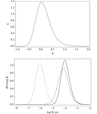
Figure 11.— Top panel: Rate ambiguity function ${\cal A}$ implied by the scaling relations and luminosity model uncertainties listed in Eq. (A1), shown versus $X$ (a dimensionless variable corresponding to logarithmic rate differences $\log R/R_{o}$). Bottom panel: our best estimates for the birthrate of tight PSR-NS (solid), wide PSR-NS (dotted), and tight PSR-WD binaries (dashed) including marginalization over alternative pulsar luminosity models. In practice, the curves shown here correspond to the thick black curves presented previously, after each has been smoothed with the kernel in the top panel. These results include the small star formation rate correction described in §2.2.

A.2. Lognormal versus Power-law

Figure 12.— Cumulative luminosity distributions $P(>L)$ for (i) the canonical power-law (solid); (ii) a lognormal distribution with $\sigma_{\log L}=0.9$ and $\left<\log L\right>=-1.1$ (dotted); and (iii) a lognormal distribution with $\left<\log L\right>=\log L_{\rm min}$ where $L_{\rm min}=0.3{\rm mJy}{\rm kpc}^{-2}$ is our fidicual cutoff for the power law distribution (dashed).

Though simple, a global power-law luminosity distribution leads to predictions that depend sensitively on the low-luminosity cutoff; see Eq. A1. Recent detailed pulsar population synthesis studies by Faucher-Giguère & Kaspi (2006) (henceforth FK) suggest a simpler, lognormal luminosity function fits the whole pulsar population

$$p(\log L)d\log L = \frac{1}{\sqrt{2\pi\sigma_{\log L}^{2}}}e^{-(\log L-<\log L>)^{2}/2\sigma_{\log L}^{2}}d\log L$$ (A8)

where $\sigma_{\log L}=0.9$; see their Fig 15. As shown in Figure 12, however, a naive lognormal distribution differs substantially from our canonical model: even adopting $\left<\log L\right>=\log 0.3\,({\rm mJy}{\rm kpc}^{-2})$, substantially larger than the best-fit model in FK with $\left<\log L\right>=-1.1$, a lognormal distribution predicts more bright and fewer faint pulsars than our fiducial power-law luminosity model. Translating to $N_{psr}$ and birthrates, compared to our fiducial power-law distribution roughly four to six times more binaries must be present in the fiducial lognormal ($\left<\log L\right>=-1.1$) for one to be detected, depending on the pulsar spin and width being simulated. For comparison, for each pulsar binary our “extreme” lognormal distribution ($\left<\log L\right>=\log 0.3$) predicts roughly the same numbers $N_{psr}$ of pulsars as the fiducial power law distribution. Further, the best fit lognormal distribution from FK is really a spin-dependent luminosity $L\propto P^{\epsilon_{P}}\dot{P}^{\epsilon_{\dot{P}}}$, with weakly constrained exponents $\epsilon_{\dot{P}}$ and $\epsilon_{P}$. That model implicitly introduces time-dependent selection effects, beyond the scope of this paper. The logormal model described above is presented as a convenient summary, not a fundamental distribution; FK thus don’t describe how reliable its parameters are. Lacking control over the model, we defer a detailed discussion of lognormal luminosity models to a future paper.

References

- Abbott, B., et al. (2008) (The LIGO Scientific Collaboration) Abbott, B., et al. (The LIGO Scientific Collaboration). 2008, Phys. Rev. D, 78, 042002
- Arzoumanian et al. (1999a) Arzoumanian, Z., Cordes, J. M., & Wasserman, I. 1999a, ApJ, 520, 696
- Arzoumanian et al. (1999b) —. 1999b, ApJ, 520, 696
- Arzoumanian et al. (1996) Arzoumanian, Z., Phillips, J. A., Taylor, J. H., & Wolszczan, A. 1996, ApJ, 470, 1111
- Aumer & Binney (2009) Aumer, M. & Binney, J. J. 2009, MNRAS, 397, 1286
- Bailes et al. (2003) Bailes, M., Ord, S. M., Knight, H. S., & Hotan, A. W. 2003, ApJ, 595, L49
- Burgay et al. (2003) Burgay, M., D’Amico, N., Possenti, A., Manchester, R. N., Lyne, A. G., Joshi, B. C., McLaughlin, M. A., Kramer, M., Sarkissian, J. M., Camilo, F., Kalogera, V., Kim, C., & Lorimer, D. R. 2003, Nature, 426, 531
- Champion et al. (2004) Champion, D. J., Lorimer, D. R., McLaughlin, M. A., Cordes, J. M., Arzoumanian, Z., Weisberg, J. M., & Taylor, J. H. 2004, MNRAS, 350, L61
- Chen & Ruderman (1993) Chen, K. & Ruderman, M. 1993, ApJ, 402, 264
- Contopoulos & Spitkovsky (2006) Contopoulos, I. & Spitkovsky, A. 2006, ApJ, 643, 1139
- Cordes & Chernoff (1997) Cordes, J. M. & Chernoff, D. F. 1997, ApJ, 482, 971
- Curran & Lorimer (1995) Curran, S. J. & Lorimer, D. R. 1995, MNRAS, 276, 347
- de la Fuente Marcos & de la Fuente Marcos (2004) de la Fuente Marcos, R. & de la Fuente Marcos, C. 2004, New Astronomy, 9, 475
- Demorest et al. (2004) Demorest, P., Ramachandran, R., Backer, D. C., Ransom, S. M., Kaspi, V., Arons, J., & Spitkovsky, A. 2004, ApJ, 615, L137
- Edwards & Bailes (2001) Edwards, R. T. & Bailes, M. 2001, ApJ, 547, L37
- Edwards et al. (2001) Edwards, R. T., Bailes, M., van Straten, W., & Britton, M. C. 2001, MNRAS, 326, 358
- Faucher-Giguère & Kaspi (2006) Faucher-Giguère, C.-A. & Kaspi, V. M. 2006, ApJ, 643, 332
- Faulkner et al. (2005) Faulkner, A. J., Kramer, M., Lyne, A. G., Manchester, R. N., McLaughlin, M. A., Stairs, I. H., Hobbs, G., Possenti, A., Lorimer, D. R., D’Amico, N., Camilo, F., & Burgay, M. 2005, ApJ, 618, L119
- Ferdman et al. (2008) Ferdman, R. D., Stairs, I. H., Kramer, M., Manchester, R. N., Lyne, A. G., Breton, R. P., McLaughlin, M. A., Possenti, A., & Burgay, M. 2008, in American Institute of Physics Conference Series, Vol. 983, 40 Years of Pulsars: Millisecond Pulsars, Magnetars and More, ed. C. Bassa, Z. Wang, A. Cumming, & V. M. Kaspi, 474
- Fuchs et al. (2009) Fuchs, B., Jahreiß, H., & Flynn, C. 2009, AJ, 137, 266
- Gil & Han (1996) Gil, J. A. & Han, J. L. 1996, ApJ, 458, 265
- Gilmore (2001) Gilmore, G. 2001, in Astronomical Society of the Pacific Conference Series, Vol. 230, Galaxy Disks and Disk Galaxies, ed. J. G. Funes & E. M. Corsini, 3–12
- Gonthier et al. (2006) Gonthier, P. L., Story, S. A., Giacherio, B. M., Arevalo, R. A., & Harding, A. K. 2006, Chinese Journal of Astronomy and Astrophysics Supplement, 6, 020000
- Gonthier et al. (2004) Gonthier, P. L., Van Guilder, R., & Harding, A. K. 2004, ApJ, 604, 775
- Harding et al. (2002) Harding, A. K., Muslimov, A. G., & Zhang, B. 2002, ApJ, 576, 366
- Hernández et al. (2001) Hernández, X., Avila-Reese, V., & Firmani, C. 2001, MNRAS, 327, 329
- Hulse & Taylor (1975) Hulse, R. A. & Taylor, J. H. 1975, ApJ, 195, L51
- Jacoby (2005) Jacoby, B. A. 2005, PhD thesis, California Institute of Technology, United States – California
- Janssen et al. (2008) Janssen, G. H., Stappers, B. W., Kramer, M., Nice, D. J., Jessner, A., Cognard, I., & Purver, M. B. 2008, A&A, 490, 753
- Johnston et al. (2008) Johnston, S., Karastergiou, A., Mitra, D., & Gupta, Y. 2008, MNRAS, 388, 261
- Kalogera et al. (2004) Kalogera, V., Kim, C., Lorimer, D. R., Burgay, M., D’Amico, N., Possenti, A., Manchester, R. N., Lyne, A. G., Joshi, B. C., McLaughlin, M. A., Kramer, M., Sarkissian, J. M., & Camilo, F. 2004, ApJ, 601, L179
- Kalogera et al. (2001) Kalogera, V., Narayan, R., Spergel, D. N., & Taylor, J. H. 2001, ApJ, 556, 340
- Kasian (2008) Kasian, L. 2008, in American Institute of Physics Conference Series, Vol. 983, 40 Years of Pulsars: Millisecond Pulsars, Magnetars and More, ed. C. Bassa, Z. Wang, A. Cumming, & V. M. Kaspi, 485–487
- Kaspi et al. (2000) Kaspi, V. M., Lyne, A. G., Manchester, R. N., Crawford, F., Camilo, F., Bell, J. F., D’Amico, N., Stairs, I. H., McKay, N. P. F., Morris, D. J., & Possenti, A. 2000, ApJ, 543, 321
- Keith et al. (2009) Keith, M. J., Kramer, M., Lyne, A. G., Eatough, R. P., Stairs, I. H., Possenti, A., Camilo, F., & Manchester, R. N. 2009, MNRAS, 393, 623
- Kim et al. (2003) Kim, C., Kalogera, V., & Lorimer, D. R. 2003, ApJ, 584, 985
- Kim et al. (2006) —. 2006, arXiv:astro-ph/0608280
- Kim et al. (2004) Kim, C., Kalogera, V., Lorimer, D. R., & White, T. 2004, ApJ, 616, 1109
- Kiziltan & Thorsett (2009) Kiziltan, B. & Thorsett, S. E. 2009, ArXiv e-prints
- Kolonko et al. (2004) Kolonko, M., Gil, J., & Maciesiak, K. 2004, A&A, 428, 943
- Kramer (2008) Kramer, M. 2008, private communication; see also Manchester et al. 2010
- Kramer et al. (2003) Kramer, M., Bell, J. F., Manchester, R. N., Lyne, A. G., Camilo, F., Stairs, I. H., D’Amico, N., Kaspi, V. M., Hobbs, G., Morris, D. J., Crawford, F., Possenti, A., Joshi, B. C., McLaughlin, M. A., Lorimer, D. R., & Faulkner, A. J. 2003, MNRAS, 342, 1299
- Kramer & Stairs (2008) Kramer, M. & Stairs, I. H. 2008, ARA&A, 46, 541
- Kramer et al. (1998) Kramer, M., Xilouris, K. M., Lorimer, D. R., Doroshenko, O., Jessner, A., Wielebinski, R., Wolszczan, A., & Camilo, F. 1998, ApJ, 501, 270
- Lorimer et al. (2007) Lorimer, D. R., Freire, P. C. C., Stairs, I. H., Kramer, M., McLaughlin, M. A., Burgay, M., Thorsett, S. E., Dewey, R. J., Lyne, A. G., Manchester, R. N., D’Amico, N., Possenti, A., & Joshi, B. C. 2007, MNRAS, 379, 1217
- Lorimer & Kramer (2004) Lorimer, D. R. & Kramer, M. 2004, Handbook of Pulsar Astronomy, ed. D. R. Lorimer & M. Kramer
- Lorimer et al. (2006) Lorimer, D. R., Stairs, I. H., Freire, P. C., Cordes, J. M., Camilo, F., Faulkner, A. J., Lyne, A. G., Nice, D. J., Ransom, S. M., Arzoumanian, Z., Manchester, R. N., Champion, D. J., van Leeuwen, J., Mclaughlin, M. A., Ramachandran, R., Hessels, J. W., Vlemmings, W., Deshpande, A. A., Bhat, N. D., Chatterjee, S., Han, J. L., Gaensler, B. M., Kasian, L., Deneva, J. S., Reid, B., Lazio, T. J., Kaspi, V. M., Crawford, F., Lommen, A. N., Backer, D. C., Kramer, M., Stappers, B. W., Hobbs, G. B., Possenti, A., D’Amico, N., & Burgay, M. 2006, ApJ, 640, 428
- Lundgren et al. (1995) Lundgren, S. C., Zepka, A. F., & Cordes, J. M. 1995, ApJ, 453, 419
- Lyne et al. (2004) Lyne, A. G., Burgay, M., Kramer, M., Possenti, A., Manchester, R. N., Camilo, F., McLaughlin, M. A., Lorimer, D. R., D’Amico, N., Joshi, B. C., Reynolds, J., & Freire, P. C. C. 2004, Science, 303, 1153
- Lyne et al. (2000) Lyne, A. G., Camilo, F., Manchester, R. N., Bell, J. F., Kaspi, V. M., D’Amico, N., McKay, N. P. F., Crawford, F., Morris, D. J., Sheppard, D. C., & Stairs, I. H. 2000, MNRAS, 312, 698
- Manchester et al. (2010) Manchester, R. N., Kramer, M., Stairs, I. H., & collaborators. 2010, ArXiv e-prints
- Mitra & Rankin (2002) Mitra, D. & Rankin, J. M. 2002, ApJ, 577, 322
- Naab & Ostriker (2006) Naab, T. & Ostriker, J. P. 2006, MNRAS, 366, 899
- Nakar (2007) Nakar, E. 2007, astro-ph/0701748
- Narayan et al. (1991) Narayan, R., Piran, T., & Shemi, A. 1991, ApJ, 379, L17
- Nice et al. (1996) Nice, D. J., Sayer, R. W., & Taylor, J. H. 1996, ApJ, 466, L87+
- Nice et al. (2008) Nice, D. J., Stairs, I. H., & Kasian, L. E. 2008, in American Institute of Physics Conference Series, Vol. 983, 40 Years of Pulsars: Millisecond Pulsars, Magnetars and More, ed. C. Bassa, Z. Wang, A. Cumming, & V. M. Kaspi, 453–458
- O’Shaughnessy et al. (2009) O’Shaughnessy, R., Kalogera, V., & Belcynski, K. 2009, in preparation
- O’Shaughnessy et al. (2005) O’Shaughnessy, R., Kim, C., Fragos, T., Kalogera, V., & Belczynski, K. 2005, ApJ, 633, 1076
- O’Shaughnessy et al. (2008) O’Shaughnessy, R., Kim, C., Kalogera, V., & Belczynski, K. 2008, ApJ, 672, 479
- Peters (1964) Peters, P. C. 1964, Phys. Rev. B, 136, 1224
- Phinney (1991) Phinney, E. S. 1991, ApJ, 380, L17
- Phinney & Blandford (1981) Phinney, E. S. & Blandford, R. D. 1981, MNRAS, 194, 137
- Rankin (1993) Rankin, J. M. 1993, ApJS, 85, 145
- Schoenrich & Binney (2009) Schoenrich, R. & Binney, J. 2009, ArXiv e-prints
- Stairs et al. (2002) Stairs, I. H., Thorsett, S. E., Taylor, J. H., & Wolszczan, A. 2002, ApJ, 581, 501
- Story et al. (2007) Story, S. A., Gonthier, P. L., & Harding, A. K. 2007, ApJ, 671, 713
- Tauris & Manchester (1998) Tauris, T. M. & Manchester, R. N. 1998, MNRAS, 298, 625
- Thompson et al. (2009) Thompson, T. A., Kistler, M. D., & Stanek, K. Z. 2009, (arXiv:0912.0009)
- Weisberg & Taylor (2002) Weisberg, J. M. & Taylor, J. H. 2002, ApJ, 576, 942
- Weltevrede & Johnston (2008) Weltevrede, P. & Johnston, S. 2008, MNRAS, 387, 1755
- Wex et al. (2000) Wex, N., Kalogera, V., & Kramer, M. 2000, ApJ, 528, 401
- Wolszczan (1991) Wolszczan, A. 1991, Nature, 350, 688
- Young et al. (2009) Young, M. D. T., Chan, L. S., Burman, R. R., & Blair, D. G. 2009, ArXiv e-prints
- Zhang et al. (2000) Zhang, B., Harding, A. K., & Muslimov, A. G. 2000, ApJ, 531, L135
- Zhang et al. (2003) Zhang, L., Jiang, Z.-J., & Mei, D.-C. 2003, PASJ, 55, 461