Time-Reversal Phase Transition at the Edge of 3d Topological Band Insulator

Abstract

We study the time reversal (T) symmetry breaking of 2d helical fermi liquid, with application to the edge states of 3d topological band insulators with only one two-component Dirac fermion at finite chemical potential, as well as other systems with spin-orbit coupling. The T-breaking Ising order parameter is not over-damped and the theory is different from the ordinary Hertz-Millis theory for order parameters at zero momentum. We argue that the T-breaking phase transition is an 3d Ising transition, and the quasiparticles are well-defined in the quantum critical regime.

Time reversal (T) symmetry is the key to guarantee the stability of both 2d and 3d topological insulators (TBI) Kane and Mele (2005a, b); Fu et al. (2007); Fu and Kane (2007), therefore it is meaningful to study the T-symmetry breaking in these systems. Because the bulk of TBI is always an insulator, the T-breaking transition only involves the edge states, which are gapless in a T-symmetric phase, and the spectrum opens up a gap when T is broken. The simplest version of 3d TBI has only one two-component Dirac fermion at the edge, which can be perfectly realized in materials based on $\mathrm{Bi}_{2}\mathrm{Se}_{3}$ and $\mathrm{Bi}_{2}\mathrm{Te}_{3}$ Xia et al. (2009); Hsieh et al. (2009a); Zhang et al. (2009a); Chen et al. (2009). The time reversal symmetry can either be broken explicitly by magnetic impurities, or broken spontaneously by strong enough interactions. The effects of magnetic impurities and quenched disorders on the edge states of 2d and 3d TBI has been discussed in Ref. Xu and Moore (2006); Wu et al. (2006) and Ref. Liu et al. (2009) respectively. Spontaneous T-breaking phase transition is most relevant to the transition metal version of the 3d TBI with interplay between spin-orbit coupling and strong interaction Pesin and Balents (2009), and it is the goal of the current paper.

Without loss of generality, the edge state of 3d TBI is described by the following time-reversal invariant Lagrangian Fu et al. (2007); Fu and Kane (2008):

$$L_{f}=\bar{\psi}(\gamma_{0}(i\partial_{t}-\mu)+v_{f}i\gamma_{j}\partial_{j})\psi.$$ (1)

$\gamma^{0}=\sigma^{z}$, $\gamma^{1}=i\sigma^{x}$, $\gamma^{2}=i\sigma^{y}$, $\bar{\psi}=\psi^{\dagger}\gamma^{0}$. $v_{f}$ is the fermi velocity at the Dirac point, $\mu$ is the chemical potential. The Pauli matrices in Eq. 1 represent the pseudospin, which is a combination between real spin space and orbital space. For conciseness we will call $\sigma^{a}$ the spin hereafter. The spin $\sigma^{a}$ of the electrons are perpendicular with their momenta. This helical spin alignment has been successfully observed in a recent ARPES measurement Hsieh et al. (2009b). The T-symmetry guarantees that in the Lagrangian the Dirac mass gap $\bar{\psi}\psi$ does not appear explicitly, although a mass generation can occur when the T-symmetry is spontaneously broken. The Dirac gap is simply the $z-$spin magnetization, hence the gap can be spontaneously generated with strong enough ferromagnetic interaction between $z-$component of spins: $-(\bar{\psi}\psi)_{r^{\prime}}V_{\vec{r},\vec{r}^{\prime}}(\bar{\psi}\psi)_{\vec{r}^{\prime}}$. To describe this T-breaking transition, we can define an Ising order parameter $\phi$, which couples to the Dirac fermions as

$$L = L_{f}+L_{b}+L_{bf},$$ (2)

$$L_{b} = (\partial_{t}\phi)^{2}-\sum_{i=x,y}v_{b}^{2}(\partial_{i}\phi)^{2}-r\phi^{2}-u\phi^{4},$$ (4)

$$L_{bf} = g\phi\bar{\psi}\psi.$$ (5)

$\bar{\psi}\psi$ order breaks T, and drives the edge to a quantum Hall phase. Identifying the leading spin order instability requires detailed knowledge of the fermion interaction, hence we focus on the universal physics at the quantum critical point, assuming the existence of the phase transition. In the current work we only discuss the discrete symmetry breaking, the transition with continuous symmetry breaking will be studied in another paper Xu (2009). The Lagrangian Eq. 5 can also describe the phase transition of magnetic impurities doped into the system, and the order parameter $\phi$ stands for the global magnetization of the magnetic impurities. The $u\phi^{4}$ term represents either the self-interaction between the magnetic impurities, or the higher order spin-spin interactions between helical fermions. In this paper we assume $u>0$ and large enough to ensure a second order transition.

Let us first take $\mu=0$ in Eq. 5, now this model becomes the Higgs-Yukawa model, which is believed to be equivalent to the Gross-Neveu model Gross and Neveu (1974); Wilson (1973) $L=i\bar{\psi}\gamma_{\mu}\partial_{\mu}\psi-\gamma(\bar{\psi}\psi)^{2},$ at least when $v_{f}=v_{b}$. The transition of $\phi$ is not 3d Ising transition because the coupling $g$ is relevant at the 3d Ising fixed point, based on the well-known scaling dimensions $[\psi]=1/2$, and $[\phi]=(d-1)/2+\eta/2=0.518$ at the 3d Ising fixed point Hasenbusch et al. (1999). If there are $N$ flavors of Dirac fermions, The critical exponents of this transition with large $N$ have been calculated by means of $1/N$ and $\epsilon=4-d$ expansions Zinn-Zustin (1991); Karkkainen et al. (1994); Gracey (1991, 1992), and a second order transition with non-Ising universality class was found. In our current case with $N=1$, there is no obvious small parameter to expand, we conjecture that the transition is still second order, with different universality class from the 3d Ising transition.

Let us now turn on a finite chemical potential $\mu$, but still make $\mu$ much smaller than the band-width $2\Lambda$ of the edge states. Now the edge states become a helical fermi liquid, with spins aligned parallel with its fermi surface. The tuning parameter $r$ in Eq. 5 will be renormalized by the static and uniform susceptibility of $\sigma^{z}$ of the helical fermi liquid

$$\Delta r\phi^{2}=\mathrm{Re}[\chi(0,0)]\phi^{2}\sim g^{2}(\mu-\Lambda)\phi^{2}.$$ (6)

Therefore the phase transition of $\phi$ can be driven by tuning the chemical potential $\mu$. Also, it is straightforward though a little tedious to check that the momentum and frequency dependence of $\mathrm{Re}[\chi]$ are nonsingular: $\mathrm{Re}[\chi(\omega,q)]\sim c_{0}-c_{1}\omega^{2}-c_{2}q^{2}+\cdots$.

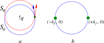
Figure 1: The fermi surface of Dirac fermions, with finite chemical potential. $a$, when we translate the fermi surface with a small momentum $\vec{q}$, at the intersection the spins are almost parallel; $b$, the two patches of fermi surface Eq. 21 describes.

As the ordinary Hert-Millis theory Hertz (1976) of quantum phase transition inside fermi liquid, the singular correction to the effective Lagrangian of order parameter comes from the imaginary part of the susceptibility. At the critical point, the critical mode of Ising order parameter $\phi$ can be damped through particle-hole excitations. The damping rate can be calculated from the Feynman diagram Fig. 2$a$, or through the Fermi-Golden rule

$$\mathrm{Im}[\Sigma_{\phi}(\omega,q)] \sim \int\frac{d^{2}k}{(2\pi)^{2}}[f(\epsilon_{k+q})-f(\epsilon_{k})]$$ (7)

$$\times \delta(|\omega|-\epsilon_{k+q}+\epsilon_{k})|\langle k|g\bar{\psi}_{k}\psi_{k+q}|k+q\rangle|^{2}$$ (9)

$$\sim \ g^{2}\frac{|\omega|q}{v_{f}k_{f}^{2}}\sqrt{1-\frac{\omega^{2}}{v_{f}^{2}q^{2}}}.$$ (11)

This result is obtained in the limit $q\ll k_{f}$, $k_{f}$ is the fermi wave-vector. When $|\omega|>v_{f}q$ the scattering rate vanishes for kinematic reasons, therefore when $v_{b}>v_{f}$ this decay rate is unimportant because the Green’s function of $\phi$ will peak when $\omega\sim v_{b}q$. From now on we will assume that $v_{b}<v_{f}$. The decay rate obtained above differs from the Hertz-Millis theory Hertz (1976) which usually takes the form $|\omega|/q$ for order parameters at zero momentum. This result can be physically understood as following: $\phi(\vec{q})$ can transfer momentum $\vec{q}$ to the fermi surface, and if we denote the fermi surface as $\mathcal{S}_{0}$, and denote the fermi surface translated by a small momentum $\vec{q}$ as $\mathcal{S}_{\vec{q}}$, then as long as $\vec{q}$ is small enough $\mathcal{S}_{\vec{q}}$ and $\mathcal{S}_{0}$ will have almost the same spin directions at their intersection. Because $\sigma^{z}$ always flips spin direction in the XY plane, when two spins are parallel the matrix element of $\sigma^{z}$ vanishes. Mathematically this intuition is manifested as $|\langle k|\bar{\psi}_{k}\psi_{k+q}|k+q\rangle|^{2}$ vanishes as $q^{2}$ in the limit of $q\rightarrow 0$. Therefore in this case $\phi$ is not overdamped at low momentum and frequency.

If we ignore the self-interaction between $\phi$, and take the Gaussian part of $L_{b}$, we can calculate the self-energy correction of fermion $\psi$ through Feynman diagram Fig. 2$b$. Evaluated close to $|\nu|\sim\epsilon_{q}$, the imaginary part of fermion self-energy scales as

$$\Sigma(\nu)^{\prime\prime} \sim \int d^{2}k\frac{1}{\omega_{k}}[\theta(\epsilon_{k+q})\delta(\nu-\epsilon_{k+q}-\omega_{k})$$ (12)

$$- \theta(-\epsilon_{k+q})\delta(\nu-\epsilon_{k+q}+\omega_{k})]$$ (14)

$$\times |\langle q|g\bar{\psi}_{q}\psi_{k+q}|k+q\rangle|^{2}\sim g^{2}\nu^{2}\mathrm{Sign}[\nu]+\cdots$$ (16)

Unlike the Hertz-Millis theory, the scaling of $\Sigma(\nu)^{\prime\prime}$ is similar to fermi liquid, which means that the quasiparticles are well-defined even at the quantum critical point.

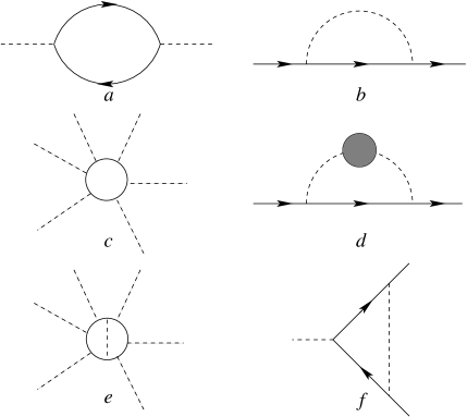
Figure 2: The one-loop Feynman diagrams for boson, fermion self-energy, vertex correction, and $\phi^{n}$ term generated with fermion loop. The dashed line and solid line represent the $\phi$ propagator and fermion propagator respectively.

The above calculations are only one-loop level. To evaluate higher loop diagrams, we had better simplify the problem by considering two patches of the fermi surface around two opposite points $(\pm k_{f},0)$, and label the fermions in terms of its momentum $p_{x}=k_{x}-k_{f}$, $p_{y}=k_{y}$. Now the action becomes

$$L_{f} = \psi^{\dagger}(\vec{p})(\omega-v_{f}p_{x}\tau^{z}-v_{y}p^{2}_{y})\psi(\vec{p}),$$ (17)

$$L_{b} = \eta\omega^{2}|\phi(\vec{p})|^{2}-(v^{2}_{bx}p^{2}_{x}+v_{by}^{2}p_{y}^{2})|\phi(\vec{p})|^{2}+\cdots$$ (19)

$$L_{bf} = igq_{y}\phi(\vec{q})\psi^{\dagger}(\vec{p})\tau^{z}\psi(\vec{p}+\vec{q})+\cdots$$ (21)

Here both $|p_{x}|$ and $|p_{y}|$ are much smaller than $k_{f}$, and $v_{y}=v_{f}/(2k_{f})$. $\tau^{z}$ is the Pauli matrix operating on the space of two fermi patches $(\pm k_{f},0)$. This isolated patch approximation is based on the observation that $\phi_{\vec{q}}$ most strongly couples to the patch with $\vec{q}\perp\vec{K}_{f}$, where the particle-hole excitation with momentum $\vec{q}$ is soft. Also, at low energy limit, none of the scattering process will mix these fermions with those from other patches. For instance, if we integrate out the boson $\phi_{\vec{q}}$, interaction between different patches will be induced, but the standard scaling argument for ordinary fermi liquid suggests that the only important interaction at low energy has $\vec{q}=0$ $i.e.$ the $\delta n_{\theta}\delta n_{\theta^{\prime}}$ interaction. However, when $\vec{q}=0$ the interaction vertex vanishes. Therefore the isolated patch approximation is reasonable.

Under discrete symmetry transformations $\mathrm{T}$, $\mathrm{P}_{x}$ and $\mathrm{P}_{y}$, the physical quantities in Eq. 21 transform as

$$\mathrm{T} : \ t\rightarrow-t,\ \psi\rightarrow\tau^{x}\psi,\ k_{i}\rightarrow-k_{i},\ \phi\rightarrow-\phi,\ i\rightarrow-i,$$ (22)

$$\mathrm{P}_{x} : \ x\rightarrow-x,\ \psi\rightarrow\tau^{x}\psi,\ k_{x}\rightarrow-k_{x},\ \phi\rightarrow-\phi,$$ (23)

$$\mathrm{P}_{y} : \ y\rightarrow-y,\ \psi\rightarrow\psi,\ k_{y}\rightarrow-k_{y},\ \phi\rightarrow-\phi.$$ (24)

and the action is invariant. Had we only kept one single fermi patch at $(+k_{f},0)$ like Ref. Polchinski (1994); Lee (2009), the action would not be invariant under these discrete transformations.

The fermion-boson vertex is proportional to $q_{y}$ of $\phi$, therefore for any loop diagram with $\phi$ external line, the loop diagram will vanish as $q_{y}\rightarrow 0$ for each $\phi$ external line. There are two different ways to assign scaling dimensions to operators in Eq. 21:

$$\mathrm{Scaling} \mathbf{1},\ [\omega]=1,\ [p_{x}]=1,\ [p_{y}]=1,\ [v_{y}]=-1,$$ (25)

$$[\phi] = -\frac{5}{2},\ [\psi]=-2,\ [\eta]=[v_{bx}]=[v_{by}]=0,$$ (26)

$$[g] = -\frac{1}{2},$$ (27)

$$\mathrm{Scaling} \mathbf{2},\ [\omega]=2,\ [p_{x}]=2,\ [p_{y}]=1,\ [v_{y}]=0,$$ (29)

$$[\phi] = [\psi]=-\frac{7}{2},\ [\eta]=[v_{bx}^{2}]=-2,\ [v_{by}^{2}]=0,$$ (30)

$$[g] = -\frac{1}{2}.$$ (31)

For both scaling choices, $[g]<0$, $i.e.$ according to the naive scaling the coupling between fermions and bosons are irrelevant, and the loop diagrams are suppressed. When we evaluate loop integrals, irrelevant terms can in general be ignored, but in order to avoid divergence from integrating a constant, we have to make a diagram-dependent choice of scaling from the two options in Eq. 31, otherwise some irrelevant terms have to be kept in the integral. For instance, we can reproduce the results obtained previously from scaling argument: at the $g^{2}$ order, choosing the second scaling in Eq. 31, the self-energy correction of $\phi$ should have dimension 3, which is consistent with the direct calculation with action Eq. 21 and Feynman diagram Fig. 2$a$:

$$\mathrm{Im}[\Sigma_{\phi}]\sim g^{2}|\omega||q_{y}|,$$ (32)

which due to energy conservation is valid when $|\omega-v_{f}q_{x}|<v_{f}|q_{y}|$. For the fermion self-energy, in order to avoid naive divergence one has to choose the first set of scaling dimensions, $[g^{2}]=-1$ implies that the self-energy should have dimension 2, which is consistent with the result $\Sigma(\nu)^{\prime\prime}\sim g^{2}\nu^{2}$ we obtained before. The one loop vertex correction can be calculated using the second scaling and Fig. 2$f$, the result is $V_{q}\sim q_{y}^{2}/(|q_{y}|+cg^{2}|\omega|)$.

Now let us discuss the nature of the T-breaking transition. The pure boson Lagrangian $L_{b}$ in Eq. 5 describes a 3d Ising transition. At the $g^{2}$ order the perturbation at the 3d Ising transition is included in the self-energy correction to $\phi$, whose singular contribution is in the imaginary part. The imaginary part of the self-energy is given by both Eq. 11 and Eq. 32, evaluated with the the full fermi surface and isolated patch approximation respectively. In both cases this self-energy mix $\phi$ at distinct points in space-time, their actual scaling dimensions at the 3D Ising critical point can be estimated as $D-(2+D-2+\eta)=-\eta$, $\eta\sim 0.037$ Hasenbusch et al. (1999). Therefore at the $g^{2}$ order there is no relevant perturbation induced at the 3d Ising fixed point.

The higher loop diagrams are more complicated, although in the previous paragraph we showed that in both choices of scalings $g$ is irrelevant, it does not immediately imply none of the higher order loops can generate important terms at the 3d Ising fixed point. This is because when we evaluate the fermi loop, in order to avoid naive divergence we have to take the second scaling in Eq. 31, which is different from the 3d Ising fixed point with isotropic scaling dimensions in space-time. For instance the leading $\phi^{n}$ term generated at $g^{n}$ order perturbation is given by diagram Fig. 2$c$, which should take the form

$$g^{n}\prod_{i=1}^{n}[q_{i,y}\phi(\vec{q}_{i})]\times f_{n}(\omega_{j},\vec{q}_{j}).$$ (33)

Notice that all the $\phi^{n}$ terms with $n$ odd are forbidden by symmetry. This term is irrelevant based on the second scaling of Eq. 31, but in order to know its scaling dimension at the 3d Ising fixed point, we need to evaluate its form more explicitly. The function $f(\omega_{j},\vec{q}_{j})$ is integral of the following fermion loop:

$$f_{n}(\omega_{j},\vec{q}_{j})\sim\int d\omega dp_{x}dp_{y}\times\delta(\sum\omega_{j})\delta(\sum\vec{q}_{j})$$ (34)

$$\times\mathrm{Tr}[\prod_{j=1}^{n}G(\omega+\sum_{i=1}^{j}\omega_{i},\vec{p}+\sum_{i=1}^{j}\vec{q}_{i})].$$ (35)

After the integral, this term has a very complicated dependence of the external frequency $\omega_{j}$ and momentum $\vec{p}_{j}$, but since we are only interested in its scaling dimension, the following schematic form will be good enough:

$$f_{n}\sim\sum\frac{|\Omega|}{\sum|Q_{y}|\prod_{j=1}^{n-2}(\Omega_{j}+v_{f}Q_{jx})+\cdots}.$$ (36)

$\Omega$ and $Q$ represent linear combination between external frequency and momentum $q$ respectively. In the denominator, the ellipses include terms with higher power of momentum compared with the leading term. We can easily verify that when $n=2$ Eq. 36 reproduces the well-known result $|\omega|/|q_{y}|$. At the 3d Gaussian fixed point, the coefficient of the $\phi^{n}$ term will have scaling dimension $1-n/2$, which should be irrelevant for any $n\geq 4$. Eq. 36 is applicable to the kinematic regime with all the external momenta nearly parallel to $\hat{y}$, when $\phi$ couples most strongly with particle-hole excitations. For more general kinematic regime the $\phi^{n}$ term generated is expected to be no more singular than Eq. 36.

So far we have only considered the leading $\phi^{n}$ term, which is generated at $g^{n}$ order. Higher order contribution to $\phi^{n}$ always involve one or more internal boson lines like Fig. 2$e$, and because of the suppression of $p_{y}$ at the internal vertices, we expect these higher order terms will not be more relevant than the leading order. For instance the result of diagram Fig. 2$e$ with one internal boson line has the same scaling dimension as Fig. 2$c$. Based on these observations, the T-breaking phase transition in the helical fermi liquid with finite $\mu$ is expected to be a 3d Ising transition. If we take into account of the interaction between $\phi$ at the 3d Ising universality class $i.e.$ using the fully dressed boson propagator in Fig. 2$d$, the self-energy of the fermion will be even more suppressed due to self-screening between bosons. One reasonable result could be $\Sigma(\nu)^{\prime\prime}\sim g^{2}|\nu|^{2+\eta}\mathrm{Sign[\nu]},$ $\eta\sim 0.037$ Hasenbusch et al. (1999) is the anomalous dimension of $\phi$ at the 3d Ising transition, since $\eta>0$, the quasiparticle is always well-defined at the quantum critical regime.

The Lagrangian Eq. 1 is invariant when spin and space are rotated by the same and arbitrary angle, which is generically larger than the symmetry of the microscopic system. For instance in material $\mathrm{Bi}_{2-x}\mathrm{Sn}_{x}\mathrm{Te}_{3}$ the fermi surface of edge states is not circular when the chemical potential is large, instead it is a hexagonal star with six sharp corners Chen et al. (2009). Therefore with large chemical potential, terms with higher order momentum should be considered in the free electron Lagrangian $L_{f}$ of Eq. 1. These higher order terms can lead to many new effects, for instance it may align the spins slightly along $\hat{z}$ direction instead of completely within the XY plane Zhang et al. (2009b); Fu (2009), although the integral of $\sigma^{z}$ vanishes along the whole fermi surface. If the spins have $\hat{z}$ component, then $\phi\sim\bar{\psi}\psi$ will cause a deformation of the fermi surface, and is overdamped for small momentum, in this case the ordinary $z=3$ Hertz-Millis theory becomes applicable.

In summary, we studied the time-reversal symmetry breaking for single Dirac fermion with finite chemical potential. Unlike the ordinary Hertz-Millis theory, the Ising order parameter is not overdamped, and we argue that the coupling between Ising order parameter and fermions is weak in the infrared limit. The transition most likely belongs to the 3d Ising universality class. The analysis in our paper can be generalized to many other systems. For instance we can consider the spin order $\psi^{\dagger}\sigma^{z}\psi$ in the Rashba model Rashba (1960); Bychkov and Rashba (1984) with inner and outer fermi surfaces with opposite inplane helical spin direction, and the results are very similar to our paper. Another system is graphene with $N=4$ flavors of Dirac fermion, our analysis applies to order parameters $\bar{\psi}\psi$ and $\bar{\psi}T^{a}\psi$ ($T^{a}\in\mathrm{SU}(N)$). For instance the phase transition of Quantum Spin Hall order $\bar{\psi}\vec{S}\psi$ belongs to the 3d O(3) universality class, when the fermi energy is tuned away from the Dirac point. In future we shall try to make connection between our results and realistic physical system, after a suitable physical system with both topological band structure and strong interaction is discovered, like the one studied theoretically in Ref. Pesin and Balents (2009).

The author appreciate the very helpful discussion with Max Metlitski and Xiaoliang Qi. This work is sponsored by the Society of Fellows, Harvard University.

References

- Kane and Mele (2005a) C. L. Kane and E. J. Mele, Phys. Rev. Lett 95, 226801 (2005a).
- Kane and Mele (2005b) C. L. Kane and E. J. Mele, Phys. Rev. Lett 95, 146802 (2005b).
- Fu et al. (2007) L. Fu, C. L. Kane, and E. J. Mele, Phys. Rev. Lett. 98, 106803 (2007).
- Fu and Kane (2007) L. Fu and C. L. Kane, Phys. Rev. B 76, 045302 (2007).
- Xia et al. (2009) Y. Xia, D. Qian, D. Hsieh, L. Wray, A. Pal, H. Lin, A. Bansil, D. Grauer, Y. S. Hor, R. J. Cava, et al., Nature Physics 5, 398 (2009).
- Hsieh et al. (2009a) D. Hsieh, Y. Xia, D. Qian, L. Wray, J. H. Dil, F. Meier, J. Osterwalder, L. Patthey, J. G. Checkelsky, N. P. Ong, et al., Nature 460, 1101 (2009a).
- Zhang et al. (2009a) H. Zhang, C.-X. Liu, X.-L. Qi, X. Dai, Z. Fang, and S.-C. Zhang, Nature Phys. 5, 438 (2009a).
- Chen et al. (2009) Y. L. Chen, J. G. Analytis, J. H. Chu, Z. K. Liu, S. K. Mo, X. L. Qi, H. J. Zhang, D. H. Lu, X. Dai, Z. Fang, et al., arXiv:0904.1829 (2009).
- Xu and Moore (2006) C. Xu and J. E. Moore, Phys. Rev. B 73, 045322 (2006).
- Wu et al. (2006) C. Wu, B. A. Bernevig, and S.-C. Zhang, Phys. Rev. Lett. 96, 106401 (2006).
- Liu et al. (2009) Q. Liu, C.-X. Liu, C. Xu, X.-L. Qi, and S.-C. Zhang, Phys. Rev. Lett. 102, 156603 (2009).
- Pesin and Balents (2009) D. A. Pesin and L. Balents, arXiv:0907.2962 (2009).
- Fu and Kane (2008) L. Fu and C. L. Kane, Phys. Rev. Lett. 100, 096407 (2008).
- Hsieh et al. (2009b) D. Hsieh, Y. Xia, D. Qian, L. Wray, J. H. Di, F. Meier, L. Patthey, J. Osterwalder, A. Fedorov, H. Lin, et al., arXiv:0904.1260 (2009b).
- Xu (2009) C. Xu, arXiv:0909.2647 (2009).
- Gross and Neveu (1974) D. Gross and A. Neveu, Phys. Rev. D 10, 3235 (1974).
- Wilson (1973) K. Wilson, Phys. Rev. D 7, 2911 (1973).
- Hasenbusch et al. (1999) M. Hasenbusch, K. Pinn, and S. Vinti, Phys. Rev. B 59, 11471 (1999).
- Zinn-Zustin (1991) J. Zinn-Zustin, Nucl. Phys. B 367, 105 (1991).
- Karkkainen et al. (1994) L. Karkkainen, R. Lacaze, P. Lacock, and B. Petersson, Nucl. Phys. B 415, 781 (1994).
- Gracey (1991) J. A. Gracey, Int. J. Mod. Phys. A 6, 395 (1991).
- Gracey (1992) J. A. Gracey, Phys. Lett. B 297, 293 (1992).
- Hertz (1976) J. A. Hertz, Phys. Rev. B 14, 1165 (1976).
- Polchinski (1994) J. Polchinski, Nucl. Phys. B 422, 617 (1994).
- Lee (2009) S.-S. Lee, arXiv: 0905.4532 (2009).
- Zhang et al. (2009b) H.-J. Zhang, C.-X. Liu, X.-L. Qi, X.-Y. Deng, X. Dai, S.-C. Zhang, and Z. Fang, arXiv:0901.2762 (2009b).
- Fu (2009) L. Fu, arXiv:0908.1418 (2009).
- Rashba (1960) E. I. Rashba, Sov. Phys. Solid State 2, 1106 (1960).
- Bychkov and Rashba (1984) Y. A. Bychkov and E. I. Rashba, J. Phys. C 17, 6039 (1984).