Supergauge interactions and electroweak baryogenesis

Abstract

We present a complete treatment of the diffusion processes for supersymmetric electroweak baryogenesis that characterizes transport dynamics ahead of the phase transition bubble wall within the symmetric phase. In particular, we generalize existing approaches to distinguish between chemical potentials of particles and their superpartners. This allows us to test the assumption of superequilibrium (equal chemical potentials for particles and sparticles) that has usually been made in earlier studies. We show that in the Minimal Supersymmetric Standard Model, superequilibrium is generically maintained – even in the absence of fast supergauge interactions – due to the presence of Yukawa interactions. We provide both analytic arguments as well as illustrative numerical examples. We also extend the latter to regions where analytical approximations are not available since down-type Yukawa couplings or supergauge interactions only incompletely equilibrate. We further comment on cases of broken superequilibrium wherein a heavy superpartner decouples from the electroweak plasma, causing a kinematic bottleneck in the chain of equilibrating reactions. Such situations may be relevant for baryogenesis within extensions of the MSSM. We also provide a compendium of inputs required to characterize the symmetric phase transport dynamics.

I Introduction

Electroweak baryogenesis (EWB) remains one of the most attractive and testable scenarios for explaining the baryon asymmetry of the universe (BAU). The BAU is characterized by the baryon number-to-entropy density ratio $Y_{B}\equiv n_{B}/s$, where $n_{B}$ is the baryon number density and $s$ is the entropy density. The value for $Y_{B}$ obtained from analysis of light element abundances in the context of Big Bang Nucleosynthesis (BBN) is consistent with the value extracted by the WMAP collaboration from acoustic peaks in the cosmic microwave background anisotropy:

$$\begin{array}[]{ccccccc}6.7\times 10^{-11}&<&Y_{B}&<&9.2\times 10^{-11}&(95\%\;\textrm{C.L.})&\textrm{BBN}\;\textnormal{\cite[cite]{\@@bibref{Authors Phrase1YearPhrase2}{Yao:2006px}{\@@citephrase{(}}{\@@citephrase{)}}}}\\ 8.36\times 10^{-11}&<&Y_{B}&<&9.32\times 10^{-11}&(95\%\;\textrm{C.L.})&\textrm{CMB}\;\textnormal{\cite[cite]{\@@bibref{Authors Phrase1YearPhrase2}{Yao:2006px,Dunkley:2008ie}{\@@citephrase{(}}{\@@citephrase{)}}}}.\end{array}$$ (1)

As observed by Sakharov Sakharov:1967dj , a particle physics explanation for this tiny number, corresponding to roughly five percent of the cosmic energy density, requires three ingredients (assuming a matter-antimatter symmetric universe at the end of inflation): (1) violation of baryon number, $B$; (2) violation of both $C$ and $CP$ symmetry; and (3) a departure from thermal equilibrium.

In EWB, these ingredients come into play if the scalar (Higgs) sector of the theory gives rise to a strongly first order electroweak phase transition (EWPT) at temperatures $T\sim 100$ GeV. Such a phase transition proceeds via bubble nucleation, wherein regions of broken electroweak symmetry emerge in a background of unbroken electroweak symmetry. $C$ and $CP$-violating interactions of fields near the bubble wall lead to the creation of left-handed charge that is injected into the unbroken phase, where electroweak sphalerons convert it into baryon number. The bubbles expand into regions of $n_{B}\not=0$, freezing it in because sphaleron transitions are quenched in the bubble interiors. A strong first order EWPT is required in order to sufficiently quench the sphalerons inside the bubble, thereby preventing wash out of the captured baryon number density.

Although the Standard Model (SM) in principle contains all the necessary ingredients for EWB, the effects of SM $CP$-violation are too suppressed to generate sufficient left-handed charge during the process of electroweak symmetry-breaking. Moreover, the LEP II lower bound on the mass of the SM Higgs boson, $m_{h}\geq 114.4$ GeV is too high to allow for a strong first order EWPT . Consequently, EWB can be viable only in the presence of new physics at the electroweak scale. In particular, augmenting the scalar sector of the SM can lead to a strong first order EWPT consistent with a SM-like Higgs scalar that is heavier than the direct search lower bound. The possibilities for doing so encompass both supersymmetric and non-supersymmetric scenarios, and in either case, searches for new scalars at the Large Hadron Collider could provide important tests (for recent work, see Refs. Menon:2009mz ; Barger:2008jx ; Noble:2007kk ; Carena:2008mj ; Barger:2007im ; Balazs:2007pf ; Profumo:2007wc and references therein). Similarly, the presence of new $CP$-violating interactions, the effects of which are not suppressed by light quark Yukawa couplings and small mixing angles as it is the case for the CKM mechanism Jarlskog:1985ht , could lead to sufficient left-handed charge generation during a first order EWPT. Experimental searches for the permanent electric dipole moments (EDMs) of the electron, neutron and neutral atoms with enhanced sensitivity could uncover the existence of such interactions Pospelov:2005pr ; Erler:2004cx ; Ramsey-Musolf:2006vr . In addition, even though other evidence for $CP$-violation may be provided by B-physics Baek:1999qy ; Hewett:2004tv (although not for the minimal field content of MSSM Murayama:2002xk ), a direct measurement of the parameters fixing the relevant $CP$-violating physics will most likely require a collider beyond LHC such as the ILC Murayama:2002xk ; Barger:2001nu . In light of these prospective experimental searches for the ingredients needed for EWB, it is important to refine the theoretical apparatus for relating their results to the baryon asymmetry.

The left-handed charge density, that biases weak sphaleron transitions and that is therefore of central relevance for the computation of the baryon asymmetry, is given by the sum of all charge densities of left-handed quarks and leptons of all generations,

$$n_{\rm left}=\sum\limits_{i=1}^{3}(q_{i}+\ell_{i})\,.$$ (2)

The number densities are understood to be the sum of both isospin components and of the three colors for the quarks. Moreover, we use the word density as a short hand expression for charge number density (the zero component of the vector current, which is the difference of particle and antiparticle number densities), and denote the densities by the symbols that also represent the particular particles. As outlined above, the left handed density gets converted into a baryon density $n_{B}$ through weak sphaleron transitions. The following formula describes baryon generation and washout ahead of the bubble wall Huet:1995sh :

$$n_{B}=-3\frac{\Gamma_{\rm ws}}{v_{\rm w}}\int\limits_{-\infty}^{0}dz\;n_{\rm left}(z){\rm e}^{\frac{15}{4}\frac{\Gamma_{\rm ws}}{v_{\rm w}}z}\,,$$ (3)

where $v_{w}$ is the bubble wall velocity and $z$ is the spatial coordinate perpendicular to the wall in the frame where the wall is at rest. Negative values of $z$ correspond to the symmetric electroweak phase (bubble exterior), positive values to the broken phase (bubble interior). Because the weak sphaleron rate, $\Gamma_{\rm ws}$, is much slower than the rates for both the creation of $n_{\mathrm{left}}$ and its diffusion ahead of the bubble wall, application of Eq. (3) is usually decoupled from the network of diffusion equations, a simplification that we also adapt here. Eq. (3) underlines the essential need of accurate theoretical methods of determining $n_{\rm left}$ in order to make quantitative predictions for $Y_{B}$.

The importance of diffusion for EWB has been emphasized in Refs. Cohen:1994ss ; Huet:1995sh ; Joyce:1994zn . Due to scatterings with the thermal bath, the $CP$-violating density $n_{\rm left}$ is not only localized at the bubble wall, but it is also transported to the region ahead of the bubble wall. Therefore, there remains a larger amount of time for weak sphaleron processes to turn $n_{\rm left}$ into the baryon asymmetry, before the it is captured by the bubble inside of which sphaleron transitions are quenched.

The purpose of the present paper is twofold: First, we present a more detailed discussion on the derivation of the diffusion equations and the computation of the interaction rates that enter these. This supplements our recent publications Chung:2008aya ; Chung:2009cb . Second, we extend the network of diffusion equations to distinguish between particle and sparticle chemical potentials. In earlier publications (see Refs. Huet:1995sh ; Chung:2008aya ; Chung:2009cb and references therein), it has been assumed that the chemical potentials for particles and their superpartners are identical, a situation that we refer to as superequilibrium. Here, we provide numerical evidence that superequilibrium holds in most regions of parameter space. On the other hand, the generalization presented here also allows for a computation of the baryon asymmetry in parametric regions where superequilibrium does not hold. As for the source of $CP$-violation, although we focus in this paper on the MSSM as an illustrative case, our methods can be applied to any supersymmetric scenario (e.g., the “next-to-minimal” Supersymmetric Standard Model).

I.1 Existing approaches to diffusion

In order to compute the left-handed charge, we need to derive and solve a coupled set of transport equations for the densities of particles that couple directly or indirectly to the $CP$-violating sources Huet:1995sh ; Joyce:1994zn :

$$\partial_{\mu}\ j_{r}^{\mu}=-\sum_{s}\Gamma_{rs}\>n_{s}+S_{r}^{\;\cancel{CP}}\ \ \ ,$$ (4)

where $j_{r}^{\mu}$ is the current density for particle species $r$, $\Gamma_{rs}$ are transport coefficients that couple the evolution of species $r$ to the number densities $n_{s}$ of other species $s$, and $S_{r}^{\;\cancel{CP}}$ is a $CP$-violating source term for the species $r$.

In earlier treatments on diffusion for EWB, it is usually assumed that the only relevant Yukawa coupling is the one of the top quark, as it is much larger than Yukawa couplings of the first generations but also much larger than third-generation couplings of down-type quarks and leptons Huet:1995sh . While we agree with the general framework for the diffusion equations and the strategies for analytical solutions that is described Ref. Huet:1995sh and followed in most subsequent work, in two recent publications Chung:2008aya ; Chung:2009cb , we have shown that the ratio between the Yukawa couplings does not directly answer the question of their relevance. Rather, the timescale associated with the interactions induced by these Yukawa couplings has to be compared to the inverse diffusion length $\Gamma_{\rm diff}^{-1}$ that is characteristic for the EWPT. In supersymmetric scenarios, the Yukawa couplings of down-type fermions and their superpartners grows with $\tan\beta$, thereby enhancing the equilibration rate for these reactions relative to diffusion. We find that for $\tan\beta\stackrel{{\scriptstyle>}}{{{}_{\sim}}}5$ ($\tan\beta\stackrel{{\scriptstyle>}}{{{}_{\sim}}}15$) interactions between bottom- ($\tau$-) particles and the Higgs sector can in general equilibrate on diffusion time-scales. This observation induces important qualitative and quantitative changes to the description of the diffusion process in EWBG:

• When bottom quark Yukawa couplings are in equilibrium, no net chemical potential associated with the axial charge of left handed third generation fermions arises. As a consequence, the production of densities of first generation quark densities through strong sphaleron processes (thermal ${\rm SU}(3)$ instantons) is suppressed.

• The sign of the baryon asymmetry depends on the sparticle mass spectrum and on $\tan\beta$, and it is therefore not uniquely given in terms of the $CP$-violating phase. In particular, in parametric regions where $\tau$-Yukawa couplings are negligible but bottom-Yukawa interactions equilibrate, the sign changes according to whether the right-handed sbottom-particle is heavier than the right handed stop or not.

• When also $\tau$-Yukawa interactions are in equilibrium, there are substantial contributions from third generation leptons to $n_{\rm left}$.

I.2 Supergauge interactions and diffusion

The particular step towards a complete treatment of the diffusion dynamics in the symmetric phase that we take in this paper is to generalize the diffusion equations to allow for different chemical potentials for particles and their superpartners, thereby accounting for possible deviations from superequilibrium. This is of importance because in supersymmetric scenarios the $CP$-violating sources generally involve interactions between supersymmetric particles and the space-time varying Higgs vacuum expectation values, leading to non-vanishing densities for the superpartners. Since the electroweak sphalerons feed on a net left-handed charge for quarks and leptons, supersymmetric interactions must efficiently transfer the non-vanishing superpartner densities into an asymmetry involving left-handed SM fermions.

In the MSSM, the most important source of left-handed charge is CP-violation in the Higgsino-gaugino sector that gives rise to a non-vanishing Higgsino density (see, e.g., Refs. Riotto:1998zb ; ewbstop ; Lee:2004we and references therein). The source $S_{\tilde{H}}^{\;\cancel{CP}}$ requires a non-vanishing phase between the supersymmetric $\mu$ parameter and the SUSY-breaking gaugino mass parameters, $M_{1,2}$. Its magnitude is largest when the difference between $\mu$ and either $M_{1}$ or $M_{2}$ is small compared to their magnitudes, leading to so-called resonant electroweak baryogenesis. In previous work, it is usually assumed that supergauge interactions , such as ${\widetilde{H}}\,{\widetilde{W}}\leftrightarrow H_{u,d}$, are sufficiently fast, that once $S_{\tilde{H}}^{\;\cancel{CP}}$ generates a non-vanishing Higgsino density, the latter immediately converts into a non-vanishing Higgs boson density. Under this assumption of gaugino-mediated superequilibrium, one may work with a total density $H$ for the Higgs bosons and their superpartners. Yukawa interactions convert the $H$ density into that for SM quarks and leptons, which are again assumed to be in equilibrium with their superpartners.

These assumptions are indeed well justified when the supergauge interactions are in equilibrium. By not distinguishing between chemical potentials of particles and their superpartners, superequilibrium has been implicitly imposed in producing the numerical results presented in Refs. Chung:2008aya ; Chung:2009cb . In this paper, we do distinguish between particle and sparticle chemical potentials and take accurate account of the finite interaction rates that tend to establish superequilibrium. In doing so, we show that:

• Superequilibrium holds in most of the relevant MSSM parameter space. We produce both analytic arguments to illustrate the reasons why and numerical studies for parameter space regions where the analytic arguments break down.

• Superequilibrium yet may be maintained when supergauge interactions are slow, either because the gauginos are heavy and decouple from the plasma or because the corresponding three-body interactions are kinematically forbidden. This preservation of superequilibrium arises through a chain of reactions involving Yukawa interactions.

• In the gaugino decoupling regime, the chain of Yukawa reactions may be broken due to the presence of addtional heavy (s)particles, leading to a departure from superequilibrium. The assumption of superequilibrium in this case may lead to an unrealistic prediction for $Y_{B}$. Such scenarios may be relevant in extensions of the MSSM that do not require light gauginos for the existence of significant CP-violating sources in the transport equations (4).

I.3 Outline of this paper

The plan of this paper is as follows: Section II, culminates in the full network of Boltzmann equations that describe diffusion, which we present in Section II.9. Leading to this, we discuss how these equations may be derived within the closed time path formalism (Section II.1), list the relevant interactions within the MSSM (Section II.2), introduce the fully thermally averaged three-body supergauge interactions (Section II.3), discuss the thermally averaged Yukawa and triscalar interactions (Section II.4) and the particular source and relaxation rates for the asymmetry (Section II.6). Additional inputs needed are thermal masses (Section II.7) and diffusion constants (Section II.8). Some simplifications in the approximation of thermal effects in the averaged interaction rates are discussed and justified in Section II.10.

In Section III, we present approximate analytical solutions to the Boltzmann equations. While in Section III.2, a brief review of the discussion in Refs. Chung:2008aya ; Chung:2009cb is provided, in Section III.1 we go beyond that and show how superequilibrium can be maintained even in case when supergauge interactions are quenched (e.g. through large gaugino masses or for kinematic reasons).

In Section IV, we provide the numerical evidence for the preceding discussions. An illustrative point in parameter space is presented, where the analytical approximation is justified and yields reasonably accurate predictions for the densities ahead of the wall (Section IV.1). By variation of $\tan\beta$, the effect of changing the strength of down-type Yukawa couplings is investigated in Section IV.2. We refer the reader to Fig. 4 which illustrate this $\tan\beta$-dependence on the relationships between chemical potentials for particles and their superpartners, and to Fig. 5, which shows the corresponding impact on the relationships between left- and right-handed Standard Model fermion chemical potentials. These figures also illustrate the impact of Yukawa-induced superequilibrium that would persist if the supergauge interaction rates were set to zero. How superequilibrium is broken and how it can be maintained in the absence of supergauge interactions is exemplified in Section IV.3. Fig. 6 summarizes the final impact on the baryon asymmetry of several of these features. There we give $Y_{B}$ as a function of $\tan\beta$ that results from the full computation with our benchmark input parameters and compare to the results that would have been obtained had we neglected the presence of supergauge interactions, the third generation lepton contributions, or departures from superequilibrium that arise at large $\tan\beta$. Conclusions are drawn in Section V.

II Diffusion transport equations

In this Section, we discuss in detail the derivation of diffusion transport equations. In comparison to earlier treatments, we generalize these equations to distinguish between particle densities and the densities of their superpartners.

II.1 Three-body rates: general formalism

We derive the diffusion transport equations for EWB using the closed time path (CTP) Schwinger-Dyson equations. Although one may use conventional kinetic theory for this purpose, we adopt the CTP framework as it allows one to systematically include higher-order corrections and the effects associated with departure from adiabatic quantum evolution (for a detailed review of the CTP framework as applied to EWB, see our earlier work in Refs. Lee:2004we ; Cirigliano:2006wh ). The CTP transport equations for bosons and fermions have the form kadanoff-baym ; Riotto:1998zb :

$$\begin{split}\frac{\partial n_{B}}{\partial X_{0}}(X)+{\mbox{\boldmath$\nabla$}}\!\cdot\!\mathbf{j}_{B}(X)=\int d^{3}z\int_{-\infty}^{X_{0}}dz_{0}\ \Bigl{[}\Sigma_{B}^{>}(X,z)G^{<}(z,X)&-G^{>}(X,z)\Sigma_{B}^{<}(z,X)\\ +G^{<}(X,z)\Sigma_{B}^{>}(z,X)&-\Sigma_{B}^{<}(X,z)G^{>}(z,X)\Bigr{]}\,,\end{split}$$ (5)

$$\begin{split}\frac{\partial n_{F}}{\partial X_{0}}(X)+{\mbox{\boldmath$\nabla$}}\!\cdot\!\mathbf{j}_{F}(X)=-\int d^{3}z\int_{-\infty}^{X_{0}}dz_{0}\ {\rm Tr}\Bigl{[}\Sigma_{F}^{>}(X,z)S^{<}(z,X)&-S^{>}(X,z)\Sigma_{F}^{<}(z,X)\\ +S^{<}(X,z)\Sigma_{F}^{>}(z,X)&-\Sigma_{F}^{<}(X,z)S^{>}(z,X)\Bigr{]}\,,\end{split}$$ (6)

where $j^{\mu}_{B}=(n_{B},{\mbox{\boldmath$j_{B}$}})$ and $j^{\mu}_{F}=(n_{F},{\mbox{\boldmath$j_{F}$}})$ are the boson and fermion current densities, respectively. The functions $G^{>,\ <}(x,y)$ and $S^{>,\ <}(x,y)$ are elements of the $2\times 2$ matrix of CTP boson and fermion propagators:

$$G^{ab}(x,y) = \langle T_{\cal P}\,\left[\phi^{a}(x)\phi^{b\,\dagger}(y)\right]\rangle\,,$$ (7)

$$S^{ab}(x,y) = \langle T_{\cal P}\,\left[\psi(x)^{a}\overline{\psi}^{b}(y)\right]\rangle\,,$$ (8)

where $\langle...\rangle$ denotes an average over the physical state of the system, $T_{\cal P}$ is a path ordering operator, and the indices $a,b$ denote the branch of a closed time integration path running from $-\infty$ to $+\infty$ (the “$+$” branch) and back to $-\infty$ (the “$-$” branch) the fields inhabit. In the case of the bosonic Greens functions, one has

$$G^{++}(x,y) \equiv G^{t}(x,y)=\langle T\,\left[\phi(x)\phi^{\dagger}(y)\right]\rangle\,,$$ (9)

$$G^{+-}(x,y) \equiv G^{<}(x,y)=\langle\phi^{\dagger}(y)\phi(x)\rangle\,,$$ (10)

$$G^{-+}(x,y) \equiv G^{>}(x,y)=\langle\phi(x)\phi^{\dagger}(y)\rangle\,,$$ (11)

$$G^{--}(x,y) \equiv G^{\bar{t}}(x,y)=\langle\bar{T}\,\left[\phi(x)\phi^{\dagger}(y)\right]\rangle\,,$$ (12)

while the corresponding expressions for the elements of $S^{ab}(x,y)$ contain the appropriate factors of $-1$ to account for fermion anti-commutation relations. The self energy functions $\Sigma_{B}^{>,\ <}(x,y)$ and $\Sigma_{F}^{>,\ <}(x,y)$ give the corresponding one particle irreducible corrections to the free inverse CTP propagators.

The source terms on the RHS of Eqns. (5) and (6) can be obtained by computing $\Sigma_{B}^{>,\ <}(x,y)$ and $\Sigma_{F}^{>,\ <}(x,y)$ order-by-order in perturbation theory. In general, doing so requires knowledge of the non-equilibrium distribution functions. However, the presence of a hierarchy of scales allows one to expand these functions about their equilibrium values in powers of appropriate scale ratios. As discussed in Refs. Lee:2004we ; Cirigliano:2006wh , these scales include a decoherence time, $\tau_{d}$, associated with the departure from adiabatic dynamics; a plasma time, $\tau_{p}$, associated with mixing between degenerate states in the plasma; and an intrinsic quasiparticle evolution time, $\tau_{\mathrm{int}}$, associated with the time evolution of a state of a given energy. For the dynamics of the electroweak plasma, one finds that $\tau_{\mathrm{int}}\ll\tau_{p}\ll\tau_{d}$, leading to a natural expansion in the scale ratios: $\varepsilon_{d}\equiv\tau_{\mathrm{int}}/\tau_{d}\sim v_{w}k_{\mathrm{eff}}/\omega$ and $\varepsilon_{p}\equiv\tau_{\mathrm{int}}/\tau_{p}\sim\Gamma_{p}/\omega$ with $v_{w}$ being the bubble wall expansion velocity, $k_{\mathrm{eff}}^{-1}$ being an effective length scale (such as the wall thickness), $\Gamma_{p}$ being a thermal quasiparticle “damping rate” in the plasma, and $\omega$ being the quasiparticle frequency. Here, we include in the damping rate any an process involving emission and absorption from the thermal bath. In addition, the plasma is relatively dilute, so that the ratio of chemical potentials to temperature, $\varepsilon_{\mu}=\mu/T$, provides an additional expansion parameter.

In terms of the $\varepsilon$ parameters, the leading contributions to the RHS of Eqns. (5) and (6) occur at $\mathcal{O}(\varepsilon^{2})$. Specifically, the $CP$-violating sources include effects of order $\varepsilon_{d}\times\varepsilon_{p}$ or $\varepsilon_{d}^{2}$, while the $CP$-conserving sources arise at order $\varepsilon_{p}\times\varepsilon_{\mu}$. In this context, the supergauge interactions generate terms of the latter type. As discussed in Refs. Lee:2004we ; Cirigliano:2006wh , the presence of the scale hierarchies embodied in the $\varepsilon$ parameters allows us to adopt the quasiparticle ansatz for the CTP Green functions and to work near chemical and kinetic equilibrium when computing these terms. To this end, we compute the the terms on the right hand side of the transport equations (5,6) following the procedure used in Ref. Cirigliano:2006wh for the calculation of the $\Gamma_{Y}$-type terms. The bosonic CTP Green functions entering the computation are given by

$$G_{i}^{>}(x,y) = \int\frac{d^{4}k}{(2\pi)^{4}}\Big{(}1+f_{B}(k_{0},\mu_{i})\Big{)}\ \rho_{i}(k_{0},{\bf k})\,,$$ (13)

$$G_{i}^{<}(x,y) = \int\frac{d^{4}k}{(2\pi)^{4}}\ f_{B}(k_{0},\mu_{i})\ \rho_{i}(k_{0},{\bf k})\,,$$ (14)

with spectral functions

$$\rho_{i}({k}_{0},\mathbf{k}) = \pi/\omega_{\bf k}\left[\delta(k^{0}-\omega_{\bf k})-\delta(k^{0}+\omega_{\bf k})\right]$$

$$= {i\over 2\omega_{k}}\biggl{[}\left({1\over{k}_{0}-\omega_{k}+i\epsilon}-{1\over{k}_{0}+\omega_{k}+i\epsilon}\right)-\left({1\over{k}_{0}-\omega_{k}-i\epsilon}-{1\over{k}_{0}+\omega_{k}-i\epsilon}\right)\biggr{]}\ \ \ ,$$

where $\omega_{\bf k}=\sqrt{{|\bf k|}^{2}+m^{2}}$. The $\rho_{i}({k}_{0},\mathbf{k})$ can be appropriately modified to take into account collision-broadening and thermal masses. Using the expansion in $\varepsilon$ parameters introduced above, it suffices to take the distribution functions to be close to the equilibrium form

$$f_{B}(k_{0},\mu_{i})=n_{B}(k_{0},\mu_{i})+{\cal O}(\varepsilon_{\rm d}/\varepsilon_{p})\,,$$ (16)

where $n_{B}(k_{0},\mu_{i})=1/[e^{(k_{0}-\mu_{i})/T}-1]$ and $\mu_{i}$ is a local chemical potential . Here we neglect the terms of order $\varepsilon_{\rm d}/\varepsilon_{p}\sim v_{w}k_{\mathrm{eff}}/\Gamma_{p}\ll 1$.

Similar expressions are obtained for the fermion Green functions:

$$S^{>}(x,y) = \langle\psi(x){\bar{\psi}}(y)\rangle\,,$$ (17)

$$S^{<}(x,y) = -\langle{\bar{\psi}}(y)\psi(x)\rangle\,,$$ (18)

which can be expressed as

$$S^{\lambda}(x,y)=\int{d^{4}k\over(2\pi)^{4}}e^{-i{k}\cdot(x-y)}f_{F}^{\lambda}({k}_{0},\mu)\rho(k_{0},\mathbf{k})\left(k\!\!\!/+m\right)\,,$$ (19)

where $\lambda$ denotes either “$>$” or “$<$” and and with the functions

$$f_{F}^{>}(k_{0},\mu) =1-n_{F}(k_{0}-\mu)\,,$$ (20a)

$$f_{F}^{<}(k_{0},\mu) =-n_{F}(k_{0}-\mu)\,,$$ (20b)

with $n_{F}(k_{0},\mu_{i})=1/[e^{(k_{0}-\mu_{i})/T}+1]$.

II.2 MSSM interaction Lagrangian

In order to calculate the transport coefficients in the Boltzmann equations, we first identify the relevant interactions in the MSSM Lagrangian. These interactions, denoted by $\mathcal{L}_{int}$, can be divided into three classes:

$$\mathcal{L}_{int}=\mathcal{L}_{M}+\mathcal{L}_{Y}+\mathcal{L}_{\widetilde{V}}\;.$$ (21)

Bilinear interactions that arise when the neutral Higgs bosons acquire vacuum expectation values (vevs) are

$$\mathcal{L}_{M}= -y_{t}\>\widetilde{t}_{R}^{*}\>\widetilde{t}_{L}\>\left(A_{t}\>v_{u}+\mu^{*}v_{d}\right)-y_{t}\>v_{u}\>\bar{t}_{R}\>P_{L}\>t_{L}$$ (22)

$$-y_{b}\>\widetilde{b}_{R}^{*}\>\widetilde{b}_{L}\>\left(A_{b}\>v_{d}+\mu^{*}v_{u}\right)-y_{b}\>v_{d}\>\bar{b}_{R}\>P_{L}\>b_{L}$$

$$-y_{\tau}\>\widetilde{\tau}_{R}^{*}\>\widetilde{\tau}_{L}\>\left(A_{\tau}\>v_{d}+\mu^{*}v_{u}\right)-y_{\tau}\>v_{d}\>\bar{\tau}_{R}\>P_{L}\>\tau_{L}$$

$$-\frac{g_{1}}{\sqrt{2}}\>\bar{\Psi}_{\widetilde{H}^{0}}(v_{d}\>P_{L}-e^{i\phi_{\mu}^{M_{1}}}v_{u}\>P_{R})\Psi_{\widetilde{B}}-\frac{g_{2}}{\sqrt{2}}\>\bar{\Psi}_{\widetilde{H}^{0}}(v_{d}\>P_{L}+e^{i\phi_{\mu}^{M_{2}}}v_{u}\>P_{R})\Psi_{\widetilde{W}^{0}}$$

$$-g_{2}\>\bar{\Psi}_{\widetilde{H}^{+}}(v_{d}\>P_{L}+e^{i\phi_{\mu}^{M_{2}}}v_{u}\>P_{R})\Psi_{\widetilde{W}^{+}}+\>\textrm{h.c.}$$

These terms, which result in squarks, quarks, sleptons, leptons and Higgsinos scattering due to the spacetime-dependent Higgs vevs $v_{u}(x)$ and $v_{d}(x)$, contribute to $CP$-violating sources $S^{\;\cancel{CP}}$ and $CP$-conserving relaxation rates $\Gamma_{M}$ and $\Gamma_{H}$. The calculation of $S^{\>\cancel{CP}}$ has received the most attention, both in the CTP approach and in other frameworks; however, there remains a significant dispersion in the recent calculations of separate groups Lee:2004we ; Carena:2002ss ; Carena:2000id ; Cline:2001rk ; Konstandin:2005cd . The $CP$-conserving relaxation rates have been estimated in Ref. Huet:1995sh , and rigorously calculated and studied with CTP methods in Ref. Lee:2004we in a manner consistent with the computation of the $CP$-violating sources.

Trilinear interactions proportional to the top Yukawa coupling $y_{t}$ are

$$\mathcal{L}_{y_{t}}= -y_{t}\>\widetilde{t}_{R}^{*}\>\widetilde{t}_{L}\>\left(A_{t}\>H_{u}^{0}+\mu^{*}H_{d}^{0*}\right)+y_{t}\>\widetilde{t}_{R}^{*}\>\widetilde{b}_{L}\>\left(A_{t}\>H_{u}^{+}-\mu^{*}H_{d}^{-*}\right)$$ (23)

$$+y_{t}\>\left(H_{u}^{+}\>\bar{t}_{R}\>P_{L}\>b_{L}-H_{u}^{0}\>\bar{t}_{R}\>P_{L}\>t_{L}\right)$$

$$+y_{t}\>e^{i\phi_{\mu}}\>\left(\widetilde{t}_{R}\>\bar{t}_{L}\>P_{R}\>\Psi_{\widetilde{H}^{0}}^{C}+\widetilde{t}_{R}\>\bar{b}_{L}\>P_{R}\>\Psi_{\widetilde{H}^{+}}^{C}\right)$$

$$+y_{t}\>e^{-i\phi_{\mu}}\>\left(\widetilde{t}_{L}\>\bar{t}_{R}\>P_{L}\>\Psi_{\widetilde{H}^{0}}+\widetilde{b}_{L}\>\bar{t}_{R}\>P_{L}\>\Psi_{\widetilde{H}^{+}}\right)\;+\;\textrm{h.c.}\;.$$

For the bottom Yukawa coupling $y_{b}$ the corresponding interactions are

$$\mathcal{L}_{y_{b}}= -y_{b}\>\widetilde{b}_{R}^{*}\>\widetilde{b}_{L}\>\left(A_{b}\>H_{d}^{0}+\mu^{*}H_{u}^{0*}\right)+y_{b}\>\widetilde{b}_{R}^{*}\>\widetilde{t}_{L}\>\left(A_{b}\>H_{d}^{-}-\mu^{*}H_{u}^{+*}\right)$$ (24)

$$+y_{b}\>\left(H_{d}^{-}\>\bar{b}_{R}\>P_{L}\>t_{L}-H_{d}^{0}\>\bar{b}_{R}\>P_{L}\>b_{L}\right)$$

$$+y_{b}\>\left(-\widetilde{b}_{R}\>\bar{b}_{L}\>P_{R}\>\Psi_{\widetilde{H}^{0}}+\widetilde{b}_{R}\>\bar{t}_{L}\>P_{R}\>\Psi_{\widetilde{H}^{+}}\right)$$

$$+y_{b}\>\left(\widetilde{b}_{L}\>\bar{b}_{R}\>P_{L}\>\Psi_{\widetilde{H}^{0}}^{C}-\widetilde{t}_{L}\>\bar{b}_{R}\>P_{L}\>\Psi_{\widetilde{H}^{+}}^{C}\right)\;+\;\textrm{h.c.}\;,$$

where we have employed notations and rephasing conventions according to Ref. Lee:2004we . The corresponding interactions $\mathcal{L}_{y_{\tau}}$ for third generation (s)leptons follow when replacing $b_{R}\to\tau_{R}$ and $t_{L}\to\nu_{\tau}$ in $\mathcal{L}_{y_{b}}$.

In general, all interactions mediated by third generation Yukawa and triscalar couplings may have a sizeable impact on the result of EWB, such that we consider

$$\mathcal{L}_{Y}=\mathcal{L}_{y_{t}}+\mathcal{L}_{y_{b}}+\mathcal{L}_{y_{\tau}}\,.$$ (25)

These terms, which are Yukawa interactions and their supersymmetric counterparts, lead to transport coefficients generically denoted $\Gamma_{Y}$. These equilibration rates are potentially important in that they communicate $CP$-asymmetries from the Higgs sector to the quark sector, biasing sphalerons to produce a baryon asymmetry. The dominant absorption/emission contribution to $\Gamma_{Y}$ has been studied within the CTP framework in Ref. Cirigliano:2006wh ; the sub-dominant scattering contribution to $\Gamma_{Y}$ has been partially calculated in Refs. Joyce:1994zn ; Huet:1995sh .

Supergauge interactions are

$$\mathcal{L}_{\widetilde{V}}= -\frac{g_{1}}{\sqrt{2}}\>\left[\bar{\Psi}_{\widetilde{H}^{+}}(H_{d}^{-*}\>P_{L}+e^{i\phi_{\mu}^{M_{1}}}H_{u}^{+}\>P_{R})\Psi_{\widetilde{B}}+\bar{\Psi}_{\widetilde{H}^{0}}(H_{d}^{0*}\>P_{L}-e^{i\phi_{\mu}^{M_{1}}}H_{u}^{0}\>P_{R})\Psi_{\widetilde{B}}\right]$$ (26)

$$-\frac{g_{2}}{\sqrt{2}}\>\left[\bar{\Psi}_{\widetilde{H}^{+}}(-H_{d}^{-*}\>P_{L}+e^{i\phi_{\mu}^{M_{2}}}H_{u}^{+}\>P_{R})\Psi_{\widetilde{W}^{0}}+\bar{\Psi}_{\widetilde{H}^{0}}(H_{d}^{0*}\>P_{L}+e^{i\phi_{\mu}^{M_{2}}}H_{u}^{0}\>P_{R})\Psi_{\widetilde{W}^{0}}\right]$$

$$-g_{2}\>\left[\bar{\Psi}_{\widetilde{H}^{+}}(H_{d}^{0*}\>P_{L}+e^{i\phi_{\mu}^{M_{2}}}H_{u}^{0}\>P_{R})\Psi_{\widetilde{W}^{+}}+\bar{\Psi}_{\widetilde{W}^{+}}(H_{d}^{-*}\>P_{L}-e^{i\phi_{\mu}^{M_{2}}}H_{u}^{+}\>P_{R})\Psi_{\widetilde{H}^{0}}^{C}\right]$$

$$-\frac{g_{2}}{\sqrt{2}}\>\left[\widetilde{u}_{L}^{i*}\>\bar{\Psi}_{\widetilde{W}^{0}}\>P_{L}\>u_{L}^{i}-\;\widetilde{d}_{L}^{i*}\>\bar{\Psi}_{\widetilde{W}^{0}}\>P_{L}\>d_{L}^{i}+\widetilde{\nu}_{L}^{i^{*}}\>\bar{\Psi}_{\widetilde{W}^{0}}P_{L}\>\nu_{L}^{i}-\widetilde{e}_{L}^{i^{*}}\>\bar{\Psi}_{\widetilde{W}^{0}}P_{L}\>e_{L}^{i}\right]$$

$$-\frac{g_{1}}{3\sqrt{2}}\>\left[\widetilde{u}_{L}^{i*}\>\bar{\Psi}_{\widetilde{B}}\>P_{L}\>u_{L}^{i}+\widetilde{d}_{L}^{i*}\>\bar{\Psi}_{\widetilde{B}}\>P_{L}\>d_{L}^{i}\right]+\frac{g_{1}}{\sqrt{2}}\>\left[\widetilde{\nu}_{L}^{i*}\bar{\Psi}_{\widetilde{B}}\>P_{L}\nu_{L}^{i}+\widetilde{e}_{L}^{i*}\bar{\Psi}_{\widetilde{B}}\>P_{L}e_{L}^{i}\right]$$

$$-g_{3}\sqrt{2}\>\left[\widetilde{u}_{L}^{i*}\>\lambda^{a}\bar{\Psi}_{\widetilde{G}}^{a}\>P_{L}\>u_{L}^{i}+\widetilde{d}_{L}^{i*}\>\lambda^{a}\>\bar{\Psi}_{\widetilde{G}}^{a}\>P_{L}\>d_{L}^{i}\right]$$

$$-g_{2}\>V_{ij}^{*}\>\widetilde{d}_{L}^{j*}\>\bar{\Psi}_{\widetilde{W}^{+}}\>P_{L}\>u_{L}^{i}-g_{2}\>V_{ij}\>\widetilde{u}_{L}^{i*}\>\bar{\Psi}_{\widetilde{W}^{+}}^{C}\>P_{L}\>d_{L}^{j}-g_{2}\>\widetilde{e}_{L}^{i*}\bar{\Psi}_{\widetilde{W}^{+}}\>P_{L}\>\nu_{L}^{i}-g_{2}\>\widetilde{\nu}_{L}^{i*}\bar{\Psi}_{\widetilde{W}^{+}}^{C}\>P_{L}\>e_{L}^{i}$$

$$-g_{3}\sqrt{2}\>\left[\widetilde{u}_{R}^{i}\>\bar{\lambda}^{a}\bar{u}_{R}^{i}P_{L}\Psi_{\widetilde{G}}^{a}+\widetilde{d}_{R}^{i}\>\bar{\lambda}^{a}\bar{d}_{R}^{i}P_{L}\Psi_{\widetilde{G}}^{a}\right]$$

$$+\;\frac{2\sqrt{2}}{3}\>g_{1}\>\left[\widetilde{u}^{i}_{R}\>\bar{u}^{i}_{R}\>P_{L}\>\Psi_{\widetilde{B}}\right]-\frac{\sqrt{2}}{3}\>g_{1}\>\left[\widetilde{d}^{i}_{R}\>\bar{d}^{i}_{R}\>P_{L}\>\Psi_{\widetilde{B}}\right]+\sqrt{2}\>g_{1}\>\left[\widetilde{e}_{R}^{i}\>\bar{e}_{R}^{i}\>P_{L}\>\Psi_{\widetilde{B}}\right]\>+\>\textrm{h.c.}\;,$$

where $\lambda^{a}$ and $\bar{\lambda}^{a}$ are the generators of $\mathbf{3}$ and $\mathbf{\bar{3}}$ of ${\rm SU}(3)$. These supergauge interactions – the supersymmetric version of gauge interactions in the SM – lead to transport coefficients, generically denoted by $\Gamma_{\widetilde{V}}$, which tend to equilibrate the chemical potentials for particles and their superpartners. All previous studies have assumed the limit $\Gamma_{\tilde{V}}\to\infty$, which leads to superequilibrium. One of the purposes of the present work is to calculate $\Gamma_{\widetilde{V}}$ and to solve the Boltzmann equations without the assumption of superequilibrium.

In employing these interactions to compute the supergauge equilibration rates, we work with the mass eigenstates of the unbroken phase: gauginos and Higgsinos (rather than charginos and neutralinos), left- and right-handed quarks and squarks, and Higgs scalars. Deep inside the bubble, this choice is clearly not appropriate, owing to large flavor mixing induced by the non-zero Higgs vevs. A proper treatment of this flavor mixing requires a modification of the transport equations that allows for an all-orders summation of the spacetime varying Higgs vevs Konstandin:2005cd ; resuminprogress . In the absence of such a treatment, we will work in the “vev insertion” approximation, defined by assuming that the dynamics of chiral charge production are dominated by the region near the phase boundary and that the Higgs vevs in this region are small compared to the temperature and slowly varying (i.e., the wall is relatively thick). Under these assumptions one may treat the flavor mixing perturbatively. We find below that the particle densities are generally largest in magnitude near the phase boundary as one would expect if the vev insertion approximation is valid. Nonetheless, we emphasize that our specific numerical conclusions are provisional and await a more complete treatment of the flavor mixing dynamics in the broken phase within the bubble.

Within the spectrum of unbroken phase eigenstates, the Higgs scalars provide additional complications. To appreciate the difficulties more clearly, suppose for simplicity the lightest Higgs mass eigenvector field $\phi$ is a fixed linear combination of $H_{u}$ and $H_{d}$ as we pass through the bubble wall. Then the naive dispersion relationship for $\phi$ modes in the WKB approximation will be

$$\omega_{\bf k}=\sqrt{|{\bf k}|^{2}+V^{\prime\prime}(\phi)}$$ (27)

where $V(\phi)$ is the thermal effective potential and $v(x)=\langle\phi\rangle$ solves the Euler-Lagrange equations involving $V^{\prime}(\phi)$ leading to the cancellation of tadpoles. For states with sufficiently large momentum, the fact that $V^{\prime\prime}(\phi)<0$ in a particular $\phi$ range will be unimportant. However, sufficiently soft modes will become unstable if $V^{\prime\prime}(\phi)<0$ and may lead to significant backreaction corrections to $v(x)$ on time scales of order $\textrm{Im}\,{\omega_{\bf k}^{-1}}$ and can also lead to particle production effects. Note that this statement of the problem is a bit more subtle than it seems because $v(x)$ is not spatially homogeneous while the thermal effective potential $V(v)$ obtained by the usual construction methods corresponds to the energy of the system with $v$ fixed to be spatially homogeneous (e.g. see Weinberg:1987vp ).

In this paper, we will simply settle with an estimate of the error incurred by neglecting this inhomogeneous bubble profile effect on the Higgs transport equations, and leave a more detailed analysis to a future work. If we denote the largest magnitude of $V^{\prime\prime}(\phi)<0$ region when the temperature is near the critical temperature $T_{c}$ as $k_{c}\equiv\max[|V^{\prime\prime}(\phi)|^{1/2}]$ , the effect of neglecting of the $V^{\prime\prime}(\phi)<0$ region on the Higgs transport equations can be estimated by the following fractional thermal distribution number density:

$$\frac{n_{c}}{n}\approx\frac{H(k_{c}/T_{c},m/T_{c})}{H(\infty,m/T_{c})}\,,$$ (28)

where

$$H(k_{c}/T,m/T)\equiv\int_{m/T}^{\sqrt{k_{c}^{2}/T^{2}+m^{2}/T^{2}}}dxx\sqrt{x^{2}-m^{2}/T^{2}}\left[\exp\left(x\right)-1\right]^{-1}$$ (29)

and where $m$ is the unbroken phase mass. The function $n_{c}/n$ is a monotonically increasing function with $k_{c}/T$ and a monotonically decreasing function with increasing $m$. Although the exact value of $k_{c}/T_{c}$ is model dependent, if we take $1\lesssim k_{c}/T_{c}\lesssim 2$ and take $m/T_{c}=0.7$, we arrive at fractional correction estimate of

$$0.09\lesssim\frac{n_{c}}{n}\lesssim 0.35.$$ (30)

Hence, we can expect order 10% of the Higgs scalar density will have significantly distorted phase space distribution due to the instability of these modes. Although not completely negligible numerically, these effects can be seen as refinements on the order unity effects presented in this paper.

In the remainder of the paper, we will make the simplifying assumption that quadratic fluctuations about the classical solution to the field equations can be approximated by a set of scalar fields $(H_{u}^{+},H_{u}^{0},H_{d}^{-},H_{d}^{0})$ with mass terms

$$\mathcal{L}\supset-\left(H_{u}^{+\dagger},H_{d}^{-}\right)\left(\begin{array}[]{cc}m_{H_{u}}^{2}+|\mu|^{2}+\delta_{u}&b+\delta_{b}\\ b+\delta_{b}&m_{H_{d}}^{2}+|\mu|^{2}+\delta_{d}\end{array}\right)\left(\begin{array}[]{c}H_{u}^{+}\\ H_{d}^{-\dagger}\end{array}\right)\;,$$ (31)

and the same for $(H_{u}^{0},H_{d}^{0\dagger})$ but with $b+\delta_{b}\to-(b+\delta_{b})$. The terms $\delta_{u,d,b}$ denote finite temperature corrections which lead to a minimum in the Higgs scalar potential at $v_{u}=v_{d}=0$. We can re-express this mass matrix using the minimization conditions for electroweak symmetry breaking at $T=0$ Martin:1997ns :

$$m_{H_{u}}^{2}+|\mu|^{2} = m_{A}^{2}\cos^{2}\beta_{0}+\frac{1}{2}m_{Z}^{2}\cos 2\beta_{0}\,,$$ (32)

$$m_{H_{d}}^{2}+|\mu|^{2} = m_{A}^{2}\sin^{2}\beta_{0}-\frac{1}{2}m_{Z}^{2}\cos 2\beta_{0}\,,$$ (33)

$$b = m_{A}^{2}\sin\beta_{0}\cos\beta_{0}\,,$$ (34)

where $m_{Z}$ and $m_{A}$ are the $Z$ and pseudoscalar Higgs boson masses at $T=0$ and

$$\tan\beta_{0}\equiv\left.\frac{v_{u}}{v_{d}}\right|_{T=0}\;.$$ (35)

Therefore, the mass term becomes

$$\mathcal{L}\supset-\left(H_{u}^{+\dagger},H_{d}^{-}\right)\left(\begin{array}[]{cc}m_{A}^{2}\cos^{2}\beta_{0}+\frac{1}{2}m_{z}^{2}\cos 2\beta_{0}+\delta_{u}&\frac{1}{2}m_{A}^{2}\sin 2\beta_{0}+\delta_{b}\\ \frac{1}{2}m_{A}^{2}\sin 2\beta_{0}+\delta_{b}&m_{A}^{2}\sin^{2}\beta_{0}-\frac{1}{2}m_{Z}^{2}\cos 2\beta_{0}+\delta_{d}\end{array}\right)\left(\begin{array}[]{c}H_{u}^{+}\\ H_{d}^{-\dagger}\end{array}\right)\;.$$ (36)

The eigenvalues, corresponding to the charged Higgs scalar masses in the unbroken phase, are

$$m_{H_{1,2}}^{2}=\frac{1}{2}\left[m_{A}^{2}+(\delta_{u}+\delta_{d})\mp\sqrt{\left((m_{A}^{2}+m_{Z}^{2})\cos 2\beta_{0}+(\delta_{u}-\delta_{d})\right)^{2}+(m_{A}^{2}\sin 2\beta_{0}+2\delta_{b})^{2}}\;\right]\;.$$ (37)

We see that if $\delta_{u,d,b}\to 0$, then $m_{H_{1}}^{2}<0$ — a consequence of the fact that electroweak symmetry is broken at low temperatures. Furthermore, the mixing angle $\alpha$, defined by

$$\left(\begin{array}[]{c}H_{u}^{+}\\ H_{d}^{-\dagger}\end{array}\right)=\left(\begin{array}[]{cc}\cos\alpha&\sin\alpha\\ -\sin\alpha&\cos\alpha\end{array}\right)\>\left(\begin{array}[]{c}H_{1}^{+}\\ H_{2}^{+}\end{array}\right)\;,$$ (38)

is given by

$$\tan 2\alpha=\frac{m_{A}^{2}\sin 2\beta_{0}+2\delta_{b}}{m_{A}^{2}\cos 2\beta_{0}+m_{Z}^{2}\cos 2\beta_{0}+\delta_{u}-\delta_{d}}\;.$$ (39)

(The neutral Higgs mass matrix differs from the charged Higgs mass matrix only by $b+\delta_{b}\to-(b+\delta_{b})$; the mass eigenvalues are the same and the mixing angle differs by an overall sign). We emphasize that we are diagonalizing the Higgs potential about its minimum at $\langle H_{u}\rangle=\langle H_{d}\rangle=0$ in the unbroken phase, as opposed to the usual zero-temperature treatment Martin:1997ns ; our results for $m_{H_{1,2}}^{2}$ and $\alpha$ do not simplify to the zero-temperature Higgs masses and mixing angles in the limit $\delta_{u,d,b}\to 0$.

If we assume that $m_{A}\gg m_{Z},\>\delta_{u,d,b}$, and $\tan\beta_{0}\gg 1$, then

$$m_{H_{1}}^{2} \simeq \delta_{u}-\frac{1}{2}m_{Z}^{2}$$ (40)

$$m_{H_{2}}^{2} \simeq m_{A}^{2}+\frac{1}{2}m_{Z}^{2}+\delta_{d}$$ (41)

and $\alpha\simeq 1/\tan\beta_{0}$. In our analysis, we will use Eq. (39). In general, this mixing angle will be spacetime-dependent due to the appearance of terms in the mass matrix proportional to $v_{u}(x),\;v_{d}(x)$. However, it has been found that

$$\Delta\beta\equiv\left.\frac{}{}\beta(T)\right|_{z\to\infty}\;-\;\left.\frac{}{}\beta(T)\right|_{z\to-\infty}$$ (42)

is numerically small: $\Delta\beta\lesssim 10^{-2}$ Moreno:1998bq . Therefore, we neglect the spacetime-dependence of the Higgs mixing angle. (In extended supersymmetric EWB scenarios, it is conceivable that $\Delta\beta$ might be larger, necessitating a proper treatment of spacetime-dependent Higgs mixing.)

The purpose of the preceding analysis is to motivate realistic masses and mixing angles in the Higgs sector. We defer a rigorous determination of Higgs boson masses and mixing during EWB to a future study.

II.3 Supergauge equilibration rates

Supergauge interactions generate three-body absorption/decay processes as illustrated in FIG. 1(a). These processes drive the plasma toward superequilibrium, the condition where the chemical potentials for a particle and its superpartner are equal. Following closely the derivation of $\Gamma_{Y}$ that is presented in Ref. Cirigliano:2006wh , we calculate the fully thermally averaged rates $\Gamma_{\widetilde{V}}$ in the on-shell limit.

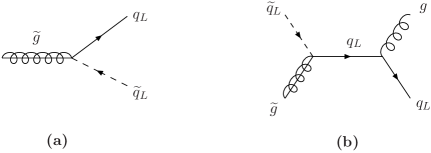
Figure 1: Examples of absorption/decay (a) and scattering (b) processes which lead to superequilibrium.

We compute the supergauge interaction rates $\Gamma_{\widetilde{V}}$ arising from emission/absorption processes in the thermal plasma [FIG. 1(a)]. Each supergauge interaction term in Eq. (26) can be cast in the general form

$$\mathcal{L}_{int}=\phi\>\bar{\psi}\left(g_{L}\,P_{L}+g_{R}\,P_{R}\right)\widetilde{V}+\;\textrm{h.c.}$$ (43)

for gaugino $\widetilde{V}$, and (bosonic, fermionic) superpartners $(\phi,\psi)$. These interactions give contributions to the RHS of Eqns. (5,6) of the form

$$\partial_{\mu}\,j_{\phi}^{\mu}(X)=-\partial_{\mu}\,j_{\psi}^{\mu}(X)=S_{\widetilde{V}}\,,$$ (44)

where

$$S_{\widetilde{V}}\equiv\left[\left(\,\left|g_{L}^{2}\right|+\left|g_{R}^{2}\right|\,\right)\>\mathcal{I}_{F}\left(m_{\psi},m_{\phi},m_{\widetilde{V}}\right)+2\,\textrm{Re}\left(g_{L}g_{R}^{*}\right)\>\widetilde{\mathcal{I}}_{F}\left(m_{\psi},m_{\phi},m_{\widetilde{V}}\right)\right]\,\left(\mu_{\psi}-\mu_{\phi}-\mu_{\widetilde{V}}\right)\;.$$ (45)

The functions $\mathcal{I}_{F}$ and $\widetilde{\mathcal{I}}_{F}$ are defined to be Cirigliano:2006wh

$$\mathcal{I}_{F}(m_{1},m_{\phi},m_{2}) =\frac{1}{16\pi^{3}T}\,\left(m_{1}^{2}+m_{2}^{2}-m_{\phi}^{2}\right)\,\int_{m_{1}}^{\infty}d\omega_{1}\int_{\omega_{\phi}^{-}}^{\omega_{\phi}^{+}}d\omega_{\phi}$$ (46)

$$\times\biggl{\{}n_{B}(\omega_{\phi}) \bigl{[}1-n_{F}(\omega_{1})\bigr{]}n_{F}(\omega_{1}-\omega_{\phi})\bigl{[}\theta(m_{1}-m_{2}-m_{\phi})-\theta(m_{\phi}-m_{1}-m_{2})\bigr{]}$$

$$\quad\qquad+n_{B}(\omega_{\phi})n_{F}(\omega_{1})\bigl{[}1-n_{F}(\omega_{1}+\omega_{\phi})\bigr{]}\theta(m_{2}-m_{1}-m_{\phi})\biggr{\}}\,,$$

with integration limits on $\omega_{\phi}$ given by

$$\begin{split}\omega_{\phi}^{\pm}=\frac{1}{2m_{1}^{2}}\Bigl{\{}&\omega_{1}\left\lvert m_{\phi}^{2}+m_{1}^{2}-m_{2}^{2}\right\rvert\\ &\pm\bigl{[}(\omega_{1}^{2}-m_{1}^{2})\bigl{(}m_{1}^{2}-(m_{2}+m_{\phi})^{2}\bigr{)}\bigl{(}m_{1}^{2}-(m_{2}-m_{\phi})^{2}\bigr{)}\bigr{]}^{1/2}\Bigl{\}};\end{split}$$ (47)

and lastly

$$\widetilde{\mathcal{I}}_{F}(m_{1},m_{\phi},m_{2})=\frac{2\,m_{1}m_{2}}{m_{1}^{2}+m^{2}_{2}-m_{\phi}^{2}}\>\mathcal{I}_{F}(m_{1},m_{\phi},m_{2})\;.$$ (48)

The gaugino chemical potential $\mu_{\widetilde{V}}$ only appears on the RHS of Eq. (45) when the gaugino is a Dirac fermion (i.e., for $\widetilde{W}^{\pm}$). For Majorana gauginos, no gaugino chemical potential appears. Although a Majorana chemical potential does not correspond to a conserved Noether current, it can arise as a deviation from a pure Fermi-Dirac distribution when annihilation processes are out of equilibrium. However, such a deviation does not contribute to Eq. (45) due to CP-symmetry. The charge current densities and corresponding chemical potentials for Dirac fermions and complex scalars are all odd under CP. However, a Majorana chemical potential is even under CP. Therefore, in the limit that we can neglect CP-violating phases in our interaction rates, Majorana chemical potentials do not contribute to the Boltzmann equations for charge current densities. We have explicitly verified that a non-vanishing Majorana chemical potential ultimately cancels from $S_{\widetilde{V}}$ to linear order in $\epsilon_{\mu}$ and at zeroth order in $CP$-violating phases $\phi_{CP}$. Physically speaking, an excess of Majorana gauginos $\widetilde{V}$ does not bias a charge asymmetry in $\psi$ and $\phi$ since the rates for $\widetilde{V}\leftrightarrow\psi\phi$ and $\widetilde{V}\leftrightarrow\bar{\psi}\phi^{\dagger}$ are equal.

At present, we work exclusively within the MSSM, where existing measurements constrain $\phi_{CP}\ll 1$; consequently, we neglect these contributions. In extensions of the MSSM where additional $CP$-violating phases are less constrained and may be large, the non-equilibrium dynamics of Majorana fermions may be important. We also emphasize that these arguments apply to the degrees of freedom that are present in the symmetric phase. This is consistent within the framework of the present paper, as our main focus is the diffusion process in the symmetric phase and as we calculate the source and relaxation terms in a pertubative mass-insertion scheme. Note that in the broken phase, the Higgsinos, which are treated as charged particles in the symmetric phase, mix e.g. with the Binos, which are Majorana particles. The resulting neutralinos are Majorana particles, but due to their Higgsino component, their out-of-equilibrium dynamics is crucial for EWB. A non-pertubative treatment of the mixing in the broken phase will be subject of future investigations.

We can relate the chemical potentials $\mu$ to charge number densities $n$ via

$$n\equiv\int\frac{d^{3}p}{(2\pi)^{3}}\left(\frac{1}{e^{(\omega_{p}-\mu)/T}\pm 1}-\frac{1}{e^{(\omega_{p}+\mu)/T}\pm 1}\right)=\frac{T^{2}}{6}\>k(m/T)\>\mu\,+\,\mathcal{O}(\epsilon_{\mu}^{3})\,,$$ (49)

where $k(m/T)$ is a statistical factor Lee:2004we

$$k(m/T)=k(0)\,\frac{c_{F,B}}{\pi^{2}}\,\int_{m/T}^{\infty}\,dx\,x\ \frac{e^{x}}{(e^{x}\pm 1)^{2}}\,\sqrt{x^{2}-m^{2}/T^{2}}\ \ \$$ (50)

with $k(0)=1$ for chiral fermions, $k(0)=2$ for Dirac fermions and complex scalars, $c_{F\,(B)}=6(3)$ for fermions (bosons), and the $+$ ($-$) sign for fermions (bosons). Therefore, we can write

$$S_{\widetilde{V}}=\Gamma_{\widetilde{V}}^{(\psi,\phi)}\>\left(\frac{n_{\psi}}{k_{\psi}}-\frac{n_{\phi}}{k_{\phi}}\right)$$ (51)

for Majorana $\widetilde{V}$, where

$$\Gamma_{\widetilde{V}}^{(\psi,\phi)}\equiv\frac{6}{T^{2}}\left[\left(\,\left|g_{L}^{2}\right|+\left|g_{R}^{2}\right|\,\right)\>\mathcal{I}_{F}\left(m_{\psi},m_{\phi},m_{\widetilde{V}}\right)+2\,\textrm{Re}\left(g_{L}g_{R}^{*}\right)\>\widetilde{\mathcal{I}}_{F}\left(m_{\psi},m_{\phi},m_{\widetilde{V}}\right)\right]\;.$$ (52)

If $\widetilde{V}$ is Dirac, as is the case for $\widetilde{W}^{\pm}$, the situation is more subtle. Instead of Eq. (51), when inserting Eq. (52) into Eq. (45), we have

$$S_{\widetilde{V}}=\Gamma_{\widetilde{V}}^{(\psi,\phi)}\>\left(\frac{n_{\psi}}{k_{\psi}}-\frac{n_{\phi}}{k_{\phi}}-\frac{n_{\widetilde{V}}}{k_{\widetilde{V}}}\right)\;,$$ (53)

meaning that that non-equilibrium dynamics of ${\widetilde{W}^{\pm}}$ does not in general decouple from the dynamics that produces $Y_{B}$. Let us consider the contributions from $S_{\widetilde{W}^{\pm}}$ to the Boltzmann equations (6) for the third generation LH quarks:

$$\partial_{\mu}j^{\mu}_{t_{L}} = -\,g_{2}^{2}\,\left|V_{tb}\right|^{2}\,\mathcal{I}_{F}(m_{t_{L}},m_{\widetilde{b}_{L}},m_{\widetilde{W}^{\pm}})\>\left(\mu_{t_{L}}-\mu_{\widetilde{b}_{L}}-\mu_{\widetilde{W}^{\pm}}\right)\,,$$ (54a)

$$\partial_{\mu}j^{\mu}_{b_{L}} = -\,g_{2}^{2}\,\left|V_{tb}\right|^{2}\,\mathcal{I}_{F}(m_{b_{L}},m_{\widetilde{t}_{L}},m_{\widetilde{W}^{\pm}})\>\left(\mu_{b_{L}}-\mu_{\widetilde{t}_{L}}+\mu_{\widetilde{W}^{\pm}}\right)\;.$$ (54b)

Now we define

$$\mu_{q} \equiv \frac{1}{2}\left(\mu_{t_{L}}+\mu_{b_{L}}\right)\,,$$ (55a)

$$\mu_{\widetilde{q}} \equiv \frac{1}{2}\left(\mu_{\widetilde{t}_{L}}+\mu_{\widetilde{b}_{L}}\right)\,,$$ (55b)

$$\Delta\mu_{q} \equiv \frac{1}{2}\left(\mu_{t_{L}}-\mu_{b_{L}}\right)\,,$$ (55c)

$$\Delta\mu_{\widetilde{q}} \equiv \frac{1}{2}\left(\mu_{\widetilde{t}_{L}}-\mu_{\widetilde{b}_{L}}\right)\;.$$ (55d)

With these definitions, we obtain from Eqns. (54)

$$\partial_{\mu}\left(j^{\mu}_{u_{L}}+j^{\mu}_{d_{L}}\right) = -\,N_{C}\,g_{2}^{2}\,\left|V_{tb}\right|^{2}\left[\mathcal{I}_{F}(m_{t_{L}},m_{\widetilde{b}_{L}},m_{\widetilde{W}^{\pm}})+\mathcal{I}_{F}(m_{b_{L}},m_{\widetilde{t}_{L}},m_{\widetilde{W}^{\pm}})\right]\left(\mu_{q}-\mu_{\widetilde{q}}\right)$$

$$-\,N_{C}\,g_{2}^{2}\,\left|V_{tb}\right|^{2}\left[\mathcal{I}_{F}(m_{t_{L}},m_{\widetilde{b}_{L}},m_{\widetilde{W}^{\pm}})-\mathcal{I}_{F}(m_{b_{L}},m_{\widetilde{t}_{L}},m_{\widetilde{W}^{\pm}})\right]\,$$

$$\qquad\qquad\qquad\times\left(\Delta\mu_{q}+\Delta\mu_{\widetilde{q}}-2\mu_{\widetilde{W}^{\pm}}\right)$$

and

$$\partial_{\mu}\left(j^{\mu}_{u_{L}}-j^{\mu}_{d_{L}}\right) = -\,N_{C}\,g_{2}^{2}\,\left|V_{tb}\right|^{2}\left[\mathcal{I}_{F}(m_{t_{L}},m_{\widetilde{b}_{L}},m_{\widetilde{W}^{\pm}})-\mathcal{I}_{F}(m_{b_{L}},m_{\widetilde{t}_{L}},m_{\widetilde{W}^{\pm}})\right]\left(\mu_{q}-\mu_{\widetilde{q}}\right)$$

$$-\,N_{C}\,g_{2}^{2}\,\left|V_{tb}\right|^{2}\left[\mathcal{I}_{F}(m_{t_{L}},m_{\widetilde{b}_{L}},m_{\widetilde{W}^{\pm}})+\mathcal{I}_{F}(m_{b_{L}},m_{\widetilde{t}_{L}},m_{\widetilde{W}^{\pm}})\right]\,$$

$$\qquad\qquad\qquad\times\left(\Delta\mu_{q}+\Delta\mu_{\widetilde{q}}-2\mu_{\widetilde{W}^{\pm}}\right)$$

In the unbroken phase, where $v_{u}=v_{d}=0$, we have $m_{t_{L}}(T)=m_{b_{L}}(T)\equiv m_{q}$ and $m_{\widetilde{t}_{L}}(T)=m_{\widetilde{b}_{L}}(T)\equiv m_{\widetilde{q}}$, so that the differences

$$\left[\mathcal{I}_{F}(m_{t_{L}},m_{\widetilde{b}_{L}},m_{\widetilde{W}^{\pm}})-\mathcal{I}_{F}(m_{b_{L}},m_{\widetilde{t}_{L}},m_{\widetilde{W}^{\pm}})\right]\longrightarrow 0\;,$$ (58)

while the sums

$$\left[\mathcal{I}_{F}(m_{t_{L}},m_{\widetilde{b}_{L}},m_{\widetilde{W}^{\pm}})+\mathcal{I}_{F}(m_{b_{L}},m_{\widetilde{t}_{L}},m_{\widetilde{W}^{\pm}})\right]\longrightarrow 2\,\mathcal{I}_{F}(m_{q},m_{\widetilde{q}},m_{\widetilde{W}^{\pm}})\;.$$ (59)

Therefore, to the extent that we can neglect isospin-violating mass differences within the bubble, isovector asymmetries such as $\Delta\mu_{q}$ decouple from isoscalar densities such as $\mu_{q}$. Although we have chosen only only one interaction as an illustration, we have verified that the decoupling of isoscalar and isovector densities occurs for all Yukawa and supergauge interactions (23, 26). Since $Y_{B}$ is produced by weak sphalerons sourced by the chiral asymmetry

$$n_{\rm left}\equiv\sum_{i=1}^{3}\left(n_{u_{L}^{i}}+n_{d_{L}^{i}}\right)\;,$$ (60)

itself an iso-scalar density, isospin-violating asymmetries decouple from the determination $Y_{B}$. In particular, $n_{\widetilde{W}^{\pm}}$ only couples to isospin-violating asymmetries and will decouple from the dynamics of $n_{\rm left}$. Therefore, we consider the closed set of Boltzmann equations for the following twenty-five densities:

$$H_{1,2} \equiv n_{H_{1,2}^{+}}+n_{H_{1,2}^{0}}\,, \widetilde{H} \equiv n_{\widetilde{H}^{+}}+n_{\widetilde{H}^{0}}\,,$$ (61a)

$$q_{1,2} \equiv n_{u^{1,2}_{L}}+n_{d^{1,2}_{L}}\,, \widetilde{q}_{1,2} \equiv n_{\widetilde{u}^{1,2}_{L}}+n_{\widetilde{d}^{1,2}_{L}}\,,$$ (61b)

$$q \equiv q_{3}\equiv n_{t_{L}}+n_{b_{L}}\,, \widetilde{q} \equiv\widetilde{q}_{3}\equiv n_{\widetilde{t}_{L}}+n_{\widetilde{b}_{L}}\,,$$ (61c)

$$u_{1,2} \equiv n_{u^{1,2}_{R}}\,, \widetilde{u}_{1,2} \equiv n_{\widetilde{u}^{1,2}_{R}}\,,$$ (61d)

$$t \equiv u_{3}\equiv n_{t_{R}}\,, \widetilde{t} \equiv\widetilde{u}_{3}\equiv n_{\widetilde{t}_{R}}\,,$$ (61e)

$$d_{1,2} \equiv n_{d^{1,2}_{R}}\,, \widetilde{d}_{1,2} \equiv n_{\widetilde{d}^{1,2}_{R}}\,,$$ (61f)

$$b \equiv d_{3}\equiv n_{b_{R}}\,, \widetilde{b} \equiv\widetilde{d}_{2}\equiv n_{\widetilde{b}_{R}}\,.$$ (61g)

$$\ell \equiv\ell_{3}\equiv n_{\tau_{L}}+n_{\nu^{\tau}_{L}}\,, \widetilde{\ell} \equiv\widetilde{\ell}_{3}\equiv n_{\widetilde{\tau}_{L}}+n_{\widetilde{\nu}^{\tau}_{L}}\,,$$ (61h)

$$\tau \equiv n_{\tau_{R}}\,, \widetilde{\tau} \equiv n_{\widetilde{\tau}_{R}}\,.$$ (61i)

We defer to future work the study of isospin breaking effects within the bubble wall which couple isospin-violating asymmetries to those listed above. Note that within the context of non-supersymmetric models, a study of deviation from isospin equilibrium has been performed and the effect has been found to be quantitatively relevant Ref:IsoEquilibrium .

The supergauge equilibration rates that enter the Boltzmann equations for these densities (61) are

$$\Gamma_{\widetilde{V}}^{(H_{1},\widetilde{H})} = \frac{6\,g_{1}^{2}}{T^{2}}\,\left[\mathcal{I}_{F}(m_{\widetilde{H}},m_{H_{1}},m_{\widetilde{B}})-\sin 2\alpha\,\widetilde{\mathcal{I}}_{F}(m_{\widetilde{H}},m_{H_{1}},m_{\widetilde{B}})\right]$$

$$+\;\frac{18\,g^{2}_{2}}{T^{2}}\,\left[\mathcal{I}_{F}(m_{\widetilde{H}},m_{H_{1}},m_{\widetilde{W}})+\sin 2\alpha\,\widetilde{\mathcal{I}}_{F}(m_{\widetilde{H}},m_{H_{1}},m_{\widetilde{W}})\right]\,,$$

$$\Gamma_{\widetilde{V}}^{(H_{2},\widetilde{H})} = \frac{6\,g_{1}^{2}}{T^{2}}\,\left[\mathcal{I}_{F}(m_{\widetilde{H}},m_{H_{2}},m_{\widetilde{B}})+\sin 2\alpha\,\widetilde{\mathcal{I}}_{F}(m_{\widetilde{H}},m_{H_{2}},m_{\widetilde{B}})\right]$$

$$+\;\frac{18\,g^{2}_{2}}{T^{2}}\,\left[\mathcal{I}_{F}(m_{\widetilde{H}},m_{H_{2}},m_{\widetilde{W}})-\sin 2\alpha\,\widetilde{\mathcal{I}}_{F}(m_{\widetilde{H}},m_{H_{2}},m_{\widetilde{W}})\right]\,,$$

$$\Gamma_{\widetilde{V}}^{(q,\widetilde{q})} = \frac{2\,N_{C}\,g_{1}^{2}}{3\,T^{2}}\,\mathcal{I}_{F}(m_{q},m_{\widetilde{q}},m_{\widetilde{B}})+\frac{18\,N_{C}\,g_{2}^{2}}{T^{2}}\,\mathcal{I}_{F}\left(m_{q},m_{\widetilde{q}},m_{\widetilde{W}}\right)$$

$$+\frac{12(N_{C}^{2}-1)\,g^{2}_{3}}{T^{2}}\,\mathcal{I}_{F}\left(m_{q},m_{\widetilde{q}},m_{\widetilde{G}}\right)\,,$$

$$\Gamma_{\widetilde{V}}^{(u,\widetilde{u})} = \frac{16\,N_{C}\,g^{2}_{1}}{3T^{2}}\mathcal{I}_{F}\left(m_{u},m_{\widetilde{u}},m_{\widetilde{B}}\right)+\frac{6(N_{C}^{2}-1)\,g_{3}^{2}}{T^{2}}\,\mathcal{I}_{F}\left(m_{u},m_{\widetilde{u}},m_{\widetilde{G}}\right)\,,$$ (62d)

$$\Gamma_{\widetilde{V}}^{(d,\widetilde{d})} = \frac{4\,N_{C}\,g_{1}^{2}}{3T^{2}}\,\mathcal{I}_{F}\left(m_{d},m_{\widetilde{d}},m_{\widetilde{B}}\right)+\frac{6(N_{C}^{2}-1)\,g_{3}^{2}}{T^{2}}\,\mathcal{I}_{F}\left(m_{d},m_{\widetilde{d}},m_{\widetilde{G}}\right)\,,$$ (62e)

$$\Gamma_{\widetilde{V}}^{(\ell,\widetilde{\ell})} = \frac{6g_{1}^{2}}{T^{2}}\mathcal{I}_{F}\left(m_{\widetilde{\ell}},m_{\ell},m_{\widetilde{B}}\right)+\frac{18g_{2}^{2}}{T^{2}}\mathcal{I}_{F}\left(m_{\widetilde{\ell}},m_{\ell},m_{\widetilde{W}}\right)\,,$$ (62f)

$$\Gamma_{\widetilde{V}}^{(\tau,\widetilde{\tau})} = \frac{12g_{1}^{2}}{T^{2}}\mathcal{I}_{F}\left(m_{\widetilde{\tau}},m_{\tau},m_{\widetilde{B}}\right)\,,$$ (62g)

where in Eqns. (62c-e) we have omitted a generational index since these expressions are identical for all generations.

II.4 Yukawa, tri-scalar, and Higgs vev induced interactions

Presently, we summarize contributions to the Boltzmann equations that arise from interactions in Eqns. (22, 23). Yukawa and SUSY-breaking tri-scalar interactions (23) lead to transport coefficients in the Boltzmann equations which couple Higgs, RH quark, and LH quark supermultiplets. We assume that the tri-scalar $A$-terms are proportional to the corresponding Yukawa coupling Martin:1997ns . For example, the term

$$\mathcal{L}_{Y}\supset y_{t}\>e^{i\phi_{\mu}}\>\left(\widetilde{t}_{R}\>\bar{t}_{L}\>P_{R}\>\Psi_{\widetilde{H}^{0}}^{C}+\widetilde{t}_{R}\>\bar{b}_{L}\>P_{R}\>\Psi_{\widetilde{H}^{+}}^{C}\right)$$ (63)

in Eq. (23) leads to a contribution to the Boltzmann equations for densities $\widetilde{t},q,\widetilde{H}$ of the form

$$\partial_{\mu}\,j^{\mu}_{\widetilde{H}}=\partial_{\mu}\,j^{\mu}_{q}=-\partial_{\mu}\,j^{\mu}_{\widetilde{t}}=\Gamma_{Y}^{(q,\widetilde{t},\widetilde{H})}\>\left(\frac{\widetilde{t}}{k_{\widetilde{t}}}-\frac{q}{k_{q}}-\frac{\widetilde{H}}{k_{\widetilde{H}}}\right)\;.$$ (64)

We now list the complete set of equilibration rates Cirigliano:2006wh arising from $\mathcal{L}_{Y}$:

$$\Gamma_{Y}^{(\widetilde{t},\widetilde{q},H_{1})} = \frac{12\,N_{C}\,y_{t}^{2}}{T^{2}}\left|\,\sin\alpha\,\mu^{*}+\cos\alpha\,A_{t}\,\right|^{2}\,\mathcal{I}_{B}\left(m_{\widetilde{t}},m_{\widetilde{1}},m_{H_{1}}\right)\,,$$ (65a)

$$\Gamma_{Y}^{(\widetilde{t},\widetilde{q},H_{2})} = \frac{12\,N_{C}\,y_{t}^{2}}{T^{2}}\left|\,\cos\alpha\,\mu^{*}-\sin\alpha\,A_{t}\,\right|^{2}\,\mathcal{I}_{B}\left(m_{\widetilde{t}},m_{\widetilde{q}},m_{H_{2}}\right)\,,$$ (65b)

$$\Gamma_{Y}^{(\widetilde{t},q,\widetilde{H})} = \frac{12\,N_{C}\,y_{t}^{2}}{T^{2}}\>\mathcal{I}_{F}\left(m_{\widetilde{H}},m_{\widetilde{t}},m_{q}\right)\,,$$ (65c)

$$\Gamma_{Y}^{(t,q,H_{1})} = \frac{12\,N_{C}\,y_{t}^{2}}{T^{2}}\,\cos^{2}\alpha\,\mathcal{I}_{F}\left(m_{t},m_{q},m_{H_{1}}\right)\,,$$ (65d)

$$\Gamma_{Y}^{(t,q,H_{2})} = \frac{12\,N_{C}\,y_{t}^{2}}{T^{2}}\,\sin^{2}\alpha\,\mathcal{I}_{F}\left(m_{t},m_{q},m_{H_{2}}\right)\,,$$ (65e)

$$\Gamma_{Y}^{(t,\widetilde{q},\widetilde{H})} = \frac{12\,N_{C}\,y_{t}^{2}}{T^{2}}\,\mathcal{I}_{F}\left(m_{t},m_{\widetilde{H}},m_{\widetilde{q}}\right)\,;$$ (65f)

$$\Gamma_{Y}^{(\widetilde{b},\widetilde{q},H_{1})} = \frac{12\,N_{C}\,y_{b}^{2}}{T^{2}}\left|\,\cos\alpha\,\mu^{*}-\sin\alpha\,A_{b}\,\right|^{2}\,\mathcal{I}_{B}\left(m_{\widetilde{b}},m_{\widetilde{q}},m_{H_{1}}\right)\,,$$ (65g)

$$\Gamma_{Y}^{(\widetilde{b},\widetilde{q},H_{2})} = \frac{12\,N_{C}\,y_{b}^{2}}{T^{2}}\left|\,\sin\alpha\,\mu^{*}+\cos\alpha\,A_{b}\,\right|^{2}\,\mathcal{I}_{B}\left(m_{\widetilde{b}},m_{\widetilde{q}},m_{H_{2}}\right)\,,$$ (65h)

$$\Gamma_{Y}^{(\widetilde{b},q,\widetilde{H})} = \frac{12\,N_{C}\,y_{b}^{2}}{T^{2}}\>\mathcal{I}_{F}\left(m_{\widetilde{H}},m_{\widetilde{b}},m_{q}\right)\,,$$ (65i)

$$\Gamma_{Y}^{(b,q,H_{1})} = \frac{12\,N_{C}\,y_{b}^{2}}{T^{2}}\,\sin^{2}\alpha\,\mathcal{I}_{F}\left(m_{b},m_{q},m_{H_{1}}\right)\,,$$ (65j)

$$\Gamma_{Y}^{(b,q,H_{2})} = \frac{12\,N_{C}\,y_{b}^{2}}{T^{2}}\,\cos^{2}\alpha\,\mathcal{I}_{F}\left(m_{b},m_{q},m_{H_{2}}\right)\,,$$ (65k)

$$\Gamma_{Y}^{(b,\widetilde{q},\widetilde{H})} = \frac{12\,N_{C}\,y_{b}^{2}}{T^{2}}\,\mathcal{I}_{F}\left(m_{b},m_{\widetilde{H}},m_{\widetilde{q}}\right)\,;$$ (65l)

$$\Gamma_{Y}^{(\widetilde{\tau},\widetilde{\ell},H_{1})} = \frac{12\,N_{C}\,y_{\tau}^{2}}{T^{2}}\left|\,\cos\alpha\,\mu^{*}-\sin\alpha\,A_{\tau}\,\right|^{2}\,\mathcal{I}_{B}\left(m_{\widetilde{\tau}},m_{\widetilde{\ell}},m_{H_{1}}\right)\,,$$ (65m)

$$\Gamma_{Y}^{(\widetilde{\tau},\widetilde{\ell},H_{2})} = \frac{12\,N_{C}\,y_{\tau}^{2}}{T^{2}}\left|\,\sin\alpha\,\mu^{*}+\cos\alpha\,A_{\tau}\,\right|^{2}\,\mathcal{I}_{B}\left(m_{\widetilde{\tau}},m_{\widetilde{\ell}},m_{H_{2}}\right)\,,$$ (65n)

$$\Gamma_{Y}^{(\widetilde{\tau},\ell,\widetilde{H})} = \frac{12\,N_{C}\,y_{\tau}^{2}}{T^{2}}\>\mathcal{I}_{F}\left(m_{\widetilde{H}},m_{\widetilde{\tau}},m_{\ell}\right)\,,$$ (65o)

$$\Gamma_{Y}^{(\tau,\ell,H_{1})} = \frac{12\,N_{C}\,y_{\tau}^{2}}{T^{2}}\,\sin^{2}\alpha\,\mathcal{I}_{F}\left(m_{\tau},m_{\ell},m_{H_{1}}\right)\,,$$ (65p)

$$\Gamma_{Y}^{(\tau,\ell,H_{2})} = \frac{12\,N_{C}\,y_{\tau}^{2}}{T^{2}}\,\cos^{2}\alpha\,\mathcal{I}_{F}\left(m_{\tau},m_{\ell},m_{H_{2}}\right)\,,$$ (65q)

$$\Gamma_{Y}^{(\tau,\widetilde{\ell},\widetilde{H})} = \frac{12\,N_{C}\,y_{\tau}^{2}}{T^{2}}\,\mathcal{I}_{F}\left(m_{\tau},m_{\widetilde{H}},m_{\widetilde{\ell}}\right)\,,$$ (65r)

where

$$\begin{split}&\mathcal{I}_{B}(m_{R},m_{L},m_{H})=-\frac{1}{16\pi^{3}T}\,\int_{m_{R}}^{\infty}d\omega_{R}\int_{\omega_{L}^{-}}^{\omega_{L}^{+}}d\omega_{L}\\ &\ \ \ \times\biggl{\{}n_{B}(\omega_{R})\bigl{[}1+n_{B}(\omega_{L})\bigr{]}n_{B}(\omega_{L}-\omega_{R})\bigl{[}\theta(m_{R}-m_{L}-m_{H})-\theta(m_{L}-m_{R}-m_{H})\bigr{]}\\ &\qquad-n_{B}(\omega_{R})n_{B}(\omega_{L})\bigl{[}1+n_{B}(\omega_{L}+\omega_{R})\bigr{]}\theta(m_{H}-m_{R}-m_{L})\biggr{\}},\end{split}$$ (66)

with integration limits given by:

$$\begin{split}\omega_{L}^{\pm}=\frac{1}{2m_{R}^{2}}\Bigl{\{}&\omega_{R}\left\lvert m_{R}^{2}+m_{L}^{2}-m_{H}^{2}\right\rvert\\ &\pm\bigl{[}(\omega_{R}^{2}-m_{R}^{2})\bigl{(}m_{R}^{2}-(m_{L}+m_{H})^{2}\bigr{)}\bigl{(}m_{R}^{2}-(m_{L}-m_{H})^{2}\bigr{)}\bigr{]}^{1/2}\Bigl{\}}.\end{split}$$ (67)

These interactions communicate the effects of $CP$-violation from the Higgs(ino) sector to the (s)quark sector. If supergauge interactions are assumed to be in equilibrium, only the sum of $\Gamma_{Y}$ rates listed above enters the Boltzmann equations that determine $Y_{B}$. This procedure has been applied in our recent publications Chung:2008aya ; Chung:2009cb . Without this assumption, we must distinguish between each rate. For example, the rate for the transfer of $CP$-violating effects from $\widetilde{H}\to t$ (65c) will be different from the rate of transfer from $\widetilde{H}\to\widetilde{t}$ (65f); this difference may impact $Y_{B}$ if transfer between $t\leftrightarrow\widetilde{t}$ is inefficient, cf. Section IV.3.

II.5 Four-body and off-shell contributions

In addition, four-body scattering interactions, such as those illustrated in FIG. 1(b), will also contribute to the equilibration process Joyce:1994zn . Although the associated rates are phase space suppressed and are higher order in the gauge couplings than the three-body rates, they can become leading order when the three-body processes are kinematically forbidden. At the same order in gauge coupling constants, also off-shell processes contribute Arnold:2001ms ; Arnold:2003zc ; Garbrecht:2008cb , which are loop instead of phase space suppressed.

A calculation of these contributions to the interaction rates may hence be important for EWB in regions of parameter space where three body interactions are kinematically forbidden. We anticipate a full calculation that takes into account the masses in the Higgs sector and of the sfermions and the gauginos, which typically can be of the same order as the temperature, to be rather involved and do not perform it within the present work. For our parametric examples, we therefore avoid here parametric regions where three-body rates are kinematically forbidden as much as it is possible. The only exception that we make concerns the interaction between $H_{1}$, $t$ and $q$, where it is hard to avoid kinematic suppression for three-body interactions and to allow for electroweak symmetry breaking at the same time. We specify the estimate for the four-body interaction that we adopt for that case in Section IV.1.

II.6 Sources and relaxation terms

$CP$-violating sources can arise from the Lagrangian terms (22) involving squarks and Higgsinos. Physically, they correspond to $CP$-asymmetric reflection and transmission rates for squarks and Higgsinos scattering from the bubble wall. In Ref. Lee:2004we , only contributions to source terms that become resonant are calculated; off-resonance these contributions become comparable to other terms that have not been calculated. Therefore, we do not include in the Boltzmann equations the chiral relaxation rates for squarks and Higgs bosons which are non-resonant for the present choices of parameters, deferring their inclusion until a complete calculation of these rates has been accomplished. We comment on the validity of this approximation in Sec. IV. In the present work, we assume a resonant Higgsino source with $|\mu|=M_{1}=200$ GeV, which is sufficient to produce the observed BAU. The precise formula for $S^{\,\cancel{CP}}_{\widetilde{H}}$ is given in Ref. Lee:2004we .

The choice of Higgsino and Bino as the source of resonant $CP$-violation rather than of Higgsino and Wino is motivated by the recent evaluation of the two loop electric dipole moments (EDMs) of the electron and the neutron in the limit of heavy first two generation squarks and sleptons Li:2008kz . The results indicate that the size of the $CP$-violating phase between $\mu$ and $M_{1}$ is much less constrained by the non-observation of permanent EDMs than the phase between $\mu$ and $M_{2}$. Therefore, Bino-driven EWB Chung:2008aya ; Li:2008ez ; Chung:2009cb may prove to be a more viable option, particularly as the sensitivity of EDM searches improve.

In addition to the source terms, there exist chiral relaxation rates that also arise from particles scattering with the Higgs background field (22) and that tend to wash out $CP$-violating asymmetries. These processes exist in both the quark and Higgs sectors and are generically denoted as $\Gamma_{M}$ and $\Gamma_{H}$, respectively. In the present work, since we must distinguish between the densities for superpartners, we must likewise distinguish between the quark and squark contributions to $\Gamma_{M}$, and between the Higgs boson and Higgsino contributions to $\Gamma_{H}$. In the Boltzmann equations to follow, we write down terms for all relaxation rates that are possible within the broken phase, both resonant and non-resonant. For the numerical examples in Section IV however, we only include the contributions that may become resonantly enhanced: the Higgsino-Bino (Higgsino-Wino) contribution to $\Gamma_{H}$, resonantly enhanced for $|\mu|=M_{1}=200\,{\rm GeV}$, ($|\mu|=M_{2}$); and the matter fermion contributions to $\Gamma_{M}$, which are resonantly enhanced since the thermal masses satisfy the relations $|m_{q}-m_{t}|\ll T$, $|m_{q}-m_{b}|\ll T$ and $|m_{\ell}-m_{\tau}|\ll T$.

To facilitate comparison with Ref. Lee:2004we , we note that we apply the slight changes of notation $\Gamma_{H}^{\widetilde{H},\widetilde{V}}=\Gamma_{h}$, $\Gamma_{M}(t,q)=(6/T^{2})\Gamma_{t}^{-}$, $\Gamma_{M}(\widetilde{t},\widetilde{q})=(6/T^{2})\Gamma_{\widetilde{t}}^{-}$.

II.7 Thermal masses

The masses that appear in the expressions for the equilibration rates $\Gamma_{Y}$, $\Gamma_{\widetilde{V}}$, in the relaxation terms $\Gamma_{H}$ and $\Gamma_{M}$ and in the source terms $S^{\,\cancel{CP}}_{\widetilde{H}}$, are understood to include thermal corrections, which we take from Ref. Chung:2009cb , assuming light right-handed stop, sbottom and stau particles. While we treat the thermal masses as Dirac mass terms for fermions, strictly speaking, the thermal masses characterize a modification of the dispersion relation only and imply no chiral symmetry breaking in the symmetric phase. We provide a justification of this procedure through a discussion of the numerical inaccuracies that are incurred in Section II.10.

II.8 Diffusion constants

When generalizing the distribution functions $f_{B}$ and $f_{F}$ to be dependent also on the spatial momentum $\mathbf{p}$ in an anisotropic way, it is possible to derive the Fick diffusion law

$$\mathbf{X}=-D_{X}\nabla X$$ (68)

from kinetic theory, where $X^{\mu}=(X,{\mathbf{X}})$ denotes the number density current for any of the particle species considered here. The quantity $D_{X}$ is the diffusion constant for the species $X$ and can be calculated from the moments of scattering matrix elements of $X$. For our purposes, it is useful to recast the diffusion law (68) by boosting (non-relativistically) to the frame where the bubble wall is at rest as

$$\partial_{\mu}X^{\mu}=v_{w}\partial_{z}X-D_{X}\partial_{z}^{2}X\,.$$ (69)

The particular values that we use here for the diffusion constants are taken from Ref. Joyce:1994zn and are summarized in Table 1 in Section IV, where we present results from our numerical studies. As a simplification, common diffusion rates for particles and sparticles are taken, such that e.g. $D_{Q}=D_{q}=D_{\widetilde{q}}$. The physical interpretation of Eqs. (68, 69) is simple: Within the plasma, a particle gets rescattered and undergoes a random walk. These scatterings are more frequent for colored particles such as quarks than for particles that interact through electroweak and non-gauge couplings only, such as the $\tau$-lepton. Therefore, $D_{R}$ is larger than $D_{Q}$, which implies that $\tau$-leptons diffuse farther away from the bubble wall than quarks.

In Ref. Joyce:1994zn , the diffusion constants have been estimated using an incomplete set of scattering matrix elements. In particular, it has been pointed out in Ref. Arnold:2001ms ; Arnold:2003zc , that infrared sensitive $t$-channel processes have been neglected. In general, one should therefore expect an order one inaccuracy within the results of Ref. Joyce:1994zn . The results in Ref. Arnold:2001ms ; Arnold:2003zc apply however to gauge theories with massless fundamental fermions only, which is why they cannot be applied directly to sfermions and to Higgs bosons. In order to quote a value for comparison, from Ref. Arnold:2001ms ; Arnold:2003zc we infer $D_{q}=4.7/T$ for six quark flavors, while from Ref. Joyce:1994zn , we adapt $D_{Q}=D_{q}=D_{\widetilde{q}}=6/T$. In order to achieve predictions of accuracy better than order unity, it will be necessary to reevaluate the diffusion constants in the future.

II.9 Boltzmann equations

We now present the full set of Boltzmann equations:

$$\partial_{\mu}t^{\mu} =-\Gamma_{M}^{(t,q)}\left(\frac{t}{k_{t}}-\frac{q}{k_{q}}\right)-\,\Gamma_{Y}^{(t,q,H_{1})}\,\left(\frac{t}{k_{t}}-\frac{q}{k_{q}}-\frac{H_{1}}{k_{H_{1}}}\right)-\Gamma_{\widetilde{V}}^{(t,\widetilde{t})}\,\left(\frac{t}{k_{t}}-\frac{\widetilde{t}}{k_{\widetilde{t}}}\right)$$ (70a)

$$\quad-\,\Gamma_{Y}^{(t,q,H_{2})}\,\left(\frac{t}{k_{t}}-\frac{q}{k_{q}}-\frac{H_{2}}{k_{H_{2}}}\right)-\Gamma_{Y}^{(t,\widetilde{q},\widetilde{H})}\,\left(\frac{t}{k_{t}}-\frac{\widetilde{q}}{k_{\widetilde{q}}}-\frac{\widetilde{H}}{k_{\widetilde{H}}}\right)+\Gamma_{\rm ss}\,N_{5}\,,$$

$$\partial_{\mu}\widetilde{t}^{\mu} =-\Gamma_{Y}^{(\widetilde{t},\widetilde{q},H_{1})}\left(\frac{\widetilde{t}}{k_{\widetilde{t}}}-\frac{\widetilde{q}}{k_{\widetilde{q}}}-\frac{H_{1}}{k_{H_{1}}}\right)-\Gamma_{Y}^{(\widetilde{t},\widetilde{q},H_{2})}\,\left(\frac{\widetilde{t}}{k_{\widetilde{t}}}-\frac{\widetilde{q}}{k_{\widetilde{q}}}-\frac{H_{2}}{k_{H_{2}}}\right)+S^{\>\cancel{CP}}_{\widetilde{t}}$$ (70b)

$$\quad-\Gamma_{Y}^{(\widetilde{t},q,\widetilde{H})}\,\left(\frac{\widetilde{t}}{k_{\widetilde{t}}}-\frac{q}{k_{q}}-\frac{\widetilde{H}}{k_{\widetilde{H}}}\right)-\Gamma_{\widetilde{V}}^{(t,\widetilde{t})}\,\left(\frac{\widetilde{t}}{k_{\widetilde{t}}}-\frac{t}{k_{t}}\right)-\Gamma_{M}^{(\widetilde{t},\widetilde{q})}\left(\frac{\widetilde{t}}{k_{\widetilde{t}}}-\frac{\widetilde{q}}{k_{\widetilde{q}}}\right)\,,$$

$$\partial_{\mu}b^{\mu} =-\Gamma_{M}^{(b,q)}\left(\frac{b}{k_{b}}-\frac{q}{k_{q}}\right)-\,\Gamma_{Y}^{(b,q,H_{1})}\,\left(\frac{b}{k_{b}}-\frac{q}{k_{q}}+\frac{H_{1}}{k_{H_{1}}}\right)-\Gamma_{\widetilde{V}}^{(b,\widetilde{b})}\,\left(\frac{b}{k_{b}}-\frac{\widetilde{b}}{k_{\widetilde{b}}}\right)$$ (70c)

$$\quad-\,\Gamma_{Y}^{(b,q,H_{2})}\,\left(\frac{b}{k_{b}}-\frac{q}{k_{q}}+\frac{H_{2}}{k_{H_{2}}}\right)-\Gamma_{Y}^{(b,\widetilde{q},\widetilde{H})}\,\left(\frac{b}{k_{b}}-\frac{\widetilde{q}}{k_{\widetilde{q}}}+\frac{\widetilde{H}}{k_{\widetilde{H}}}\right)+\Gamma_{\rm ss}\,N_{5}\,,$$

$$\partial_{\mu}\widetilde{b}^{\mu} =-\Gamma_{Y}^{(\widetilde{b},\widetilde{q},H_{1})}\left(\frac{\widetilde{b}}{k_{\widetilde{b}}}-\frac{\widetilde{q}}{k_{\widetilde{q}}}+\frac{H_{1}}{k_{H_{1}}}\right)-\Gamma_{Y}^{(\widetilde{b},\widetilde{q},H_{2})}\,\left(\frac{\widetilde{b}}{k_{\widetilde{b}}}-\frac{\widetilde{q}}{k_{\widetilde{q}}}+\frac{H_{2}}{k_{H_{2}}}\right)+S^{\>\cancel{CP}}_{\widetilde{b}}$$ (70d)

$$\quad-\Gamma_{Y}^{(\widetilde{b},q,\widetilde{H})}\,\left(\frac{\widetilde{b}}{k_{\widetilde{b}}}-\frac{q}{k_{q}}+\frac{\widetilde{H}}{k_{\widetilde{H}}}\right)-\Gamma_{\widetilde{V}}^{(b,\widetilde{b})}\,\left(\frac{\widetilde{b}}{k_{\widetilde{b}}}-\frac{b}{k_{b}}\right)-\Gamma_{M}^{(\widetilde{b},\widetilde{q})}\left(\frac{\widetilde{b}}{k_{\widetilde{b}}}-\frac{\widetilde{q}}{k_{\widetilde{q}}}\right)\,,$$

$$\partial_{\mu}q^{\mu} =-\Gamma_{M}^{(t,q)}\left(\frac{q}{k_{q}}-\frac{t}{k_{t}}\right)-\Gamma_{M}^{(b,q)}\left(\frac{q}{k_{q}}-\frac{b}{k_{b}}\right)-\Gamma_{\widetilde{V}}^{(q,\widetilde{q})}\,\left(\frac{q}{k_{q}}-\frac{\widetilde{q}}{k_{\widetilde{q}}}\right)-2\,\Gamma_{\rm ss}\,N_{5}$$ (70e)

$$\quad-\Gamma_{Y}^{(t,q,H_{1})}\,\left(\frac{q}{k_{q}}-\frac{t}{k_{t}}+\frac{H_{1}}{k_{H_{1}}}\right)-\Gamma_{Y}^{(t,q,H_{2})}\,\left(\frac{q}{k_{q}}-\frac{t}{k_{t}}+\frac{H_{2}}{k_{H_{2}}}\right)-\Gamma_{Y}^{(\widetilde{t},q,\widetilde{H})}\left(\frac{q}{k_{q}}-\frac{\widetilde{t}}{k_{\widetilde{t}}}+\frac{\widetilde{H}}{k_{\widetilde{H}}}\right)$$

$$\quad-\Gamma_{Y}^{(b,q,H_{1})}\,\left(\frac{q}{k_{q}}-\frac{b}{k_{b}}-\frac{H_{1}}{k_{H_{1}}}\right)-\Gamma_{Y}^{(b,q,H_{2})}\,\left(\frac{q}{k_{q}}-\frac{b}{k_{b}}-\frac{H_{2}}{k_{H_{2}}}\right)-\Gamma_{Y}^{(\widetilde{b},q,\widetilde{H})}\left(\frac{q}{k_{q}}-\frac{\widetilde{b}}{k_{\widetilde{b}}}-\frac{\widetilde{H}}{k_{\widetilde{H}}}\right)\,,$$

$$\partial_{\mu}\widetilde{q}^{\mu} =-\Gamma_{M}^{(\widetilde{t},\widetilde{q})}\left(\frac{\widetilde{q}}{k_{\widetilde{q}}}-\frac{\widetilde{t}}{k_{\widetilde{t}}}\right)-\Gamma_{M}^{(\widetilde{b},\widetilde{q})}\left(\frac{\widetilde{q}}{k_{\widetilde{q}}}-\frac{\widetilde{b}}{k_{\widetilde{b}}}\right)-\Gamma_{\widetilde{V}}^{(q,\widetilde{q})}\,\left(\frac{\widetilde{q}}{k_{\widetilde{q}}}-\frac{q}{k_{q}}\right)-S^{\;\cancel{CP}}_{\widetilde{t}}-S^{\;\cancel{CP}}_{\widetilde{b}}$$ (70f)

$$\quad-\Gamma_{Y}^{(\widetilde{t},\widetilde{q},H_{1})}\,\left(\frac{\widetilde{q}}{k_{\widetilde{q}}}-\frac{\widetilde{t}}{k_{\widetilde{t}}}+\frac{H_{1}}{k_{H_{1}}}\right)-\Gamma_{Y}^{(\widetilde{t},\widetilde{q},H_{2})}\,\left(\frac{\widetilde{q}}{k_{\widetilde{q}}}-\frac{\widetilde{t}}{k_{\widetilde{t}}}+\frac{H_{2}}{k_{H_{2}}}\right)-\Gamma_{Y}^{(t,\widetilde{q},\widetilde{H})}\,\left(\frac{\widetilde{q}}{k_{\widetilde{q}}}-\frac{t}{k_{t}}+\frac{\widetilde{H}}{k_{\widetilde{H}}}\right)$$

$$\quad-\Gamma_{Y}^{(\widetilde{b},\widetilde{q},H_{1})}\,\left(\frac{\widetilde{q}}{k_{\widetilde{q}}}-\frac{\widetilde{b}}{k_{\widetilde{b}}}-\frac{H_{1}}{k_{H_{1}}}\right)-\Gamma_{Y}^{(\widetilde{b},\widetilde{q},H_{2})}\,\left(\frac{\widetilde{q}}{k_{\widetilde{q}}}-\frac{\widetilde{b}}{k_{\widetilde{b}}}-\frac{H_{2}}{k_{H_{2}}}\right)-\Gamma_{Y}^{(b,\widetilde{q},\widetilde{H})}\,\left(\frac{\widetilde{q}}{k_{\widetilde{q}}}-\frac{b}{k_{b}}-\frac{\widetilde{H}}{k_{\widetilde{H}}}\right)\,,$$

$$\partial_{\mu}\tau^{\mu} =-\Gamma_{M}^{(\tau,\ell)}\left(\frac{\tau}{k_{\tau}}-\frac{\ell}{k_{\ell}}\right)-\,\Gamma_{Y}^{(\tau,\ell,H_{1})}\,\left(\frac{\tau}{k_{\tau}}-\frac{\ell}{k_{\ell}}+\frac{H_{1}}{k_{H_{1}}}\right)-\Gamma_{\widetilde{V}}^{(\tau,\widetilde{\tau})}\,\left(\frac{\tau}{k_{\tau}}-\frac{\widetilde{\tau}}{k_{\widetilde{\tau}}}\right)$$ (70g)

$$\quad-\,\Gamma_{Y}^{(\tau,\ell,H_{2})}\,\left(\frac{\tau}{k_{\tau}}-\frac{\ell}{k_{\ell}}+\frac{H_{2}}{k_{H_{2}}}\right)-\Gamma_{Y}^{(\tau,\widetilde{\ell},\widetilde{H})}\,\left(\frac{\tau}{k_{\tau}}-\frac{\widetilde{\ell}}{k_{\widetilde{\ell}}}+\frac{\widetilde{H}}{k_{\widetilde{H}}}\right)\,,$$

$$\partial_{\mu}\widetilde{\tau}^{\mu} =-\Gamma_{Y}^{(\widetilde{\tau},\widetilde{\ell},H_{1})}\left(\frac{\widetilde{\tau}}{k_{\widetilde{\tau}}}-\frac{\widetilde{\ell}}{k_{\widetilde{\ell}}}+\frac{H_{1}}{k_{H_{1}}}\right)-\Gamma_{Y}^{(\widetilde{\tau},\widetilde{\ell},H_{2})}\,\left(\frac{\widetilde{\tau}}{k_{\widetilde{\tau}}}-\frac{\widetilde{\ell}}{k_{\widetilde{\ell}}}+\frac{H_{2}}{k_{H_{2}}}\right)+S^{\>\cancel{CP}}_{\widetilde{\tau}}$$ (70h)

$$\quad-\Gamma_{Y}^{(\widetilde{\tau},\ell,\widetilde{H})}\,\left(\frac{\widetilde{\tau}}{k_{\widetilde{\ell}}}-\frac{\ell}{k_{\ell}}+\frac{\widetilde{H}}{k_{\widetilde{H}}}\right)-\Gamma_{\widetilde{V}}^{(\tau,\widetilde{\tau})}\,\left(\frac{\widetilde{\tau}}{k_{\widetilde{\tau}}}-\frac{\tau}{k_{\tau}}\right)-\Gamma_{M}^{(\widetilde{\tau},\widetilde{\ell})}\left(\frac{\widetilde{\tau}}{k_{\widetilde{\tau}}}-\frac{\widetilde{\ell}}{k_{\widetilde{\ell}}}\right)\,,$$

$$\partial_{\mu}\ell^{\mu} =-\Gamma_{M}^{(\tau,\ell)}\left(\frac{q}{k_{q}}-\frac{\ell}{k_{\ell}}\right)-\Gamma_{\widetilde{V}}^{(\ell,\widetilde{\ell})}\,\left(\frac{\ell}{k_{\ell}}-\frac{\widetilde{\tau}}{k_{\widetilde{\tau}}}\right)$$ (70i)

$$\quad-\Gamma_{Y}^{(\tau,\ell,H_{1})}\,\left(\frac{\ell}{k_{\ell}}-\frac{\ell}{k_{\ell}}-\frac{H_{1}}{k_{H_{1}}}\right)-\Gamma_{Y}^{(\tau,\ell,H_{2})}\,\left(\frac{\ell}{k_{\ell}}-\frac{\tau}{k_{\tau}}-\frac{H_{2}}{k_{H_{2}}}\right)-\Gamma_{Y}^{(\widetilde{\tau},\ell,\widetilde{H})}\left(\frac{\ell}{k_{\ell}}-\frac{\widetilde{\tau}}{k_{\widetilde{\tau}}}-\frac{\widetilde{H}}{k_{\widetilde{H}}}\right)\,,$$

$$\partial_{\mu}\widetilde{\ell}^{\mu} =-\Gamma_{M}^{(\widetilde{\tau},\widetilde{\ell})}\left(\frac{\widetilde{\ell}}{k_{\widetilde{\ell}}}-\frac{\widetilde{\tau}}{k_{\widetilde{\tau}}}\right)-\Gamma_{\widetilde{V}}^{(\ell,\widetilde{\ell})}\,\left(\frac{\widetilde{\ell}}{k_{\widetilde{\ell}}}-\frac{\ell}{k_{\ell}}\right)-S^{\;\cancel{CP}}_{\widetilde{\tau}}$$ (70j)

$$\quad-\Gamma_{Y}^{(\widetilde{\tau},\widetilde{\ell},H_{1})}\,\left(\frac{\widetilde{\ell}}{k_{\widetilde{\ell}}}-\frac{\widetilde{\tau}}{k_{\widetilde{\tau}}}-\frac{H_{1}}{k_{H_{1}}}\right)-\Gamma_{Y}^{(\widetilde{\tau},\widetilde{\ell},H_{2})}\,\left(\frac{\widetilde{\ell}}{k_{\widetilde{\ell}}}-\frac{\widetilde{\tau}}{k_{\widetilde{\tau}}}-\frac{H_{2}}{k_{H_{2}}}\right)-\Gamma_{Y}^{(\tau,\widetilde{\ell},\widetilde{H})}\,\left(\frac{\widetilde{\ell}}{k_{\widetilde{\ell}}}-\frac{\tau}{k_{\tau}}-\frac{\widetilde{H}}{k_{\widetilde{H}}}\right)\,,$$

$$\partial_{\mu}H_{i}^{\mu} =-\Gamma_{Y}^{(t,q,H_{i})}\,\left(\frac{H_{i}}{k_{H_{i}}}-\frac{t}{k_{t}}+\frac{q}{k_{q}}\right)-\Gamma_{Y}^{(\widetilde{t},\widetilde{q},H_{1,2})}\,\left(\frac{H_{i}}{k_{H_{i}}}-\frac{\widetilde{t}}{k_{\widetilde{t}}}+\frac{\widetilde{q}}{k_{\widetilde{q}}}\right)$$ (70k)

$$\quad-\Gamma_{Y}^{(b,q,H_{i})}\,\left(\frac{H_{i}}{k_{H_{i}}}+\frac{b}{k_{b}}-\frac{q}{k_{q}}\right)-\Gamma_{Y}^{(\widetilde{b},\widetilde{q},H_{1,2})}\,\left(\frac{H_{i}}{k_{H_{i}}}+\frac{\widetilde{b}}{k_{\widetilde{b}}}-\frac{\widetilde{q}}{k_{\widetilde{q}}}\right)$$

$$\quad-\Gamma_{Y}^{(\tau,\ell,H_{i})}\,\left(\frac{H_{i}}{k_{H_{i}}}+\frac{\tau}{k_{\tau}}-\frac{\ell}{k_{\ell}}\right)-\Gamma_{Y}^{(\widetilde{\tau},\widetilde{\ell},H_{1,2})}\,\left(\frac{H_{i}}{k_{H_{i}}}+\frac{\widetilde{\tau}}{k_{\widetilde{\tau}}}-\frac{\widetilde{\ell}}{k_{\widetilde{\ell}}}\right)$$

$$\quad-\Gamma_{\widetilde{V}}^{(H_{i},\widetilde{H})}\,\left(\frac{H_{i}}{k_{H_{i}}}-\frac{\widetilde{H}}{k_{\widetilde{H}}}\right)-\Gamma_{H}^{(H_{1},H_{2})}\left(\frac{H_{i}}{k_{H_{i}}}\right)\;,\qquad i=1,2\,,$$

$$\partial_{\mu}\widetilde{H}^{\mu} =-\Gamma_{Y}^{(t,\widetilde{q},\widetilde{H})}\,\left(\frac{\widetilde{H}}{k_{\widetilde{H}}}-\frac{t}{k_{t}}+\frac{\widetilde{q}}{k_{\widetilde{q}}}\right)-\Gamma_{Y}^{(\widetilde{t},q,\widetilde{H})}\,\left(\frac{\widetilde{H}}{k_{\widetilde{H}}}-\frac{\widetilde{t}}{k_{\widetilde{t}}}+\frac{q}{k_{q}}\right)$$ (70l)

$$\quad-\Gamma_{Y}^{(b,\widetilde{q},\widetilde{H})}\,\left(\frac{\widetilde{H}}{k_{\widetilde{H}}}+\frac{b}{k_{b}}-\frac{\widetilde{q}}{k_{\widetilde{q}}}\right)-\Gamma_{Y}^{(\widetilde{b},q,\widetilde{H})}\,\left(\frac{\widetilde{H}}{k_{\widetilde{H}}}+\frac{\widetilde{b}}{k_{\widetilde{b}}}-\frac{q}{k_{q}}\right)$$

$$\quad-\Gamma_{Y}^{(\tau,\widetilde{\ell},\widetilde{H})}\,\left(\frac{\widetilde{H}}{k_{\widetilde{H}}}+\frac{\tau}{k_{\tau}}-\frac{\widetilde{\ell}}{k_{\widetilde{\ell}}}\right)-\Gamma_{Y}^{(\widetilde{\tau},\ell,\widetilde{H})}\,\left(\frac{\widetilde{H}}{k_{\widetilde{H}}}+\frac{\widetilde{\tau}}{k_{\widetilde{\tau}}}-\frac{\ell}{k_{\ell}}\right)$$

$$\quad-\Gamma_{H}^{(\widetilde{H},\widetilde{V})}\,\left(\frac{\widetilde{H}}{k_{\widetilde{H}}}\right)-\Gamma_{\widetilde{V}}^{(H_{1},\widetilde{H})}\,\left(\frac{\widetilde{H}}{k_{\widetilde{H}}}-\frac{H_{1}}{k_{H_{1}}}\right)-\Gamma_{\widetilde{V}}^{(H_{2},\widetilde{H})}\,\left(\frac{\widetilde{H}}{k_{\widetilde{H}}}-\frac{H_{2}}{k_{H_{2}}}\right)+S^{\;\cancel{CP}}_{\widetilde{H}}\,,$$

$$\partial_{\mu}q^{\mu}_{i} =-\Gamma_{\widetilde{V}}^{(q_{i},\widetilde{q}_{i})}\,\left(\frac{q_{i}}{k_{q_{i}}}-\frac{\widetilde{q}_{i}}{k_{\widetilde{q}_{i}}}\right)-2\,\Gamma_{\rm ss}\,N_{5}\;,\qquad i=1,2\,,$$ (70m)

$$\partial_{\mu}\widetilde{q}^{\mu}_{i} =-\Gamma_{\widetilde{V}}^{(q_{i},\widetilde{q}_{i})}\,\left(\frac{\widetilde{q}_{i}}{k_{\widetilde{q}_{i}}}-\frac{q_{i}}{k_{q_{i}}}\right)\;,\qquad i=1,2\,,$$ (70n)

$$\partial_{\mu}u^{\mu}_{i} =-\Gamma_{\widetilde{V}}^{(u_{i},\widetilde{u}_{i})}\,\left(\frac{u_{i}}{k_{u_{i}}}-\frac{\widetilde{u}_{i}}{k_{\widetilde{u}_{i}}}\right)+\Gamma_{\rm ss}\,N_{5}\;,\qquad i=1,2\,,$$ (70o)

$$\ \partial_{\mu}\widetilde{u}^{\mu}_{i} =-\Gamma_{\widetilde{V}}^{(u_{i},\widetilde{u}_{i})}\,\left(\frac{\widetilde{u}_{i}}{k_{\widetilde{u}_{i}}}-\frac{u_{i}}{k_{u_{i}}}\right)\;,\qquad i=1,2\,,$$ (70p)

$$\partial_{\mu}d_{i}^{\mu} =-\Gamma_{\widetilde{V}}^{(d_{i},\widetilde{d}_{i})}\,\left(\frac{d_{i}}{k_{d_{i}}}-\frac{\widetilde{d}_{i}}{k_{\widetilde{d}_{i}}}\right)+\Gamma_{\rm ss}\,N_{5}\;\qquad i=1,2\,,$$ (70q)

$$\partial_{\mu}\widetilde{d}^{\mu}_{i} =-\Gamma_{\widetilde{V}}^{(d_{i},\widetilde{d}_{i})}\,\left(\frac{\widetilde{d}_{i}}{k_{\widetilde{d}_{i}}}-\frac{d_{i}}{k_{d_{i}}}\right)\;\qquad i=1,2\,.$$ (70r)

The rate for strong sphaleron transitions is given by Giudice:1993bb ; Huet:1995sh ; Moore:1997im :

$$\Gamma_{\rm ss}=16\,\kappa_{s}\,\alpha_{s}^{4}\,T$$ (71)

with $\kappa_{s}\simeq 1$, and

$$N_{5}\equiv\sum_{i=1}^{3}\left(\frac{2\,q_{i}}{k_{q_{i}}}-\frac{u_{i}}{k_{u_{i}}}-\frac{d_{i}}{k_{d_{i}}}\right)\;.$$ (72)

In order to facilitate a comparison with results appearing previously in the literature, we give the our values for the statistical factors in the massless limit: $k_{q}=k_{\widetilde{q}}/2=6$, $k_{u_{R}}=k_{d_{R}}=k_{\widetilde{u}_{R}}/2=k_{\widetilde{d}_{R}}/2=3$, $k_{H_{1}}=k_{H_{2}}=4$ and $k_{\widetilde{H}}=4$.

Before solving the system of Boltzmann equations in Secs. III, IV, we conclude the present section by considering two issues related to the equilibration rates $\Gamma_{Y,\widetilde{V}}$ derived above. First, we consider the impact on these rates from a more rigorous treatment of massless fermion propagators in a thermal plasma. Second, we present a numerical comparison of $\Gamma_{Y}$ and $\Gamma_{\widetilde{V}}$ rates to demonstrate that one in general does not have $\Gamma_{\widetilde{V}}\gg\Gamma_{Y}$.

II.10 Thermal fermion propagators and particle/hole modes

For three-body processes involving scalars and fermions with masses of order $T$, the forms for the Greens functions given in Eqns. (13,14) (and the fermion analogs) suffice for the computation of the three-body rates. In the case of fermions that are massless (or nearly massless) at zero temperature, the structure of the thermal Greens functions becomes far more complicated. The renormalized fermionic spectral functions contain additional poles – so called “hole modes” – generated by mixing between single and multiparticle states in the thermal bath Klimov ; Weldon:1989ys . The resulting propagators are given by Weldon:1999th ; Lee:2004we

$$S^{\lambda}(x,y;\mu)=\int{d^{4}k\over(2\pi)^{4}}e^{-ik\cdot(x-y)}g_{F}^{\lambda}(k_{0},\mu)\left[\frac{\gamma_{0}-\mbox{\boldmath$\gamma$}\!\cdot\!\mathbf{\hat{k}}}{2}\rho_{+}(k_{0},\mathbf{k},\mu)+\frac{\gamma_{0}+\mbox{\boldmath$\gamma$}\!\cdot\!\mathbf{\hat{k}}}{2}\rho_{-}(k_{0},\mathbf{k},\mu)\right]\,,$$ (73)

where $\mathbf{\hat{k}}$ is the unit vector in the $\mathbf{k}$ direction, and

$$\begin{split}\rho_{+}(k_{0},\mathbf{k},\mu)=i\biggl{[}&\frac{Z_{p}(k,\mu)}{k_{0}-\mathcal{E}_{p}(k,\mu)}-\frac{Z_{p}(k,\mu)^{*}}{k_{0}-\mathcal{E}_{p}(k,\mu)^{*}}\\ +&\frac{Z_{h}(k,-\mu)^{*}}{k_{0}+\mathcal{E}_{h}(k,-\mu)^{*}}-\frac{Z_{h}(k,-\mu)}{k_{0}+\mathcal{E}_{h}(k,-\mu)}+F(k_{0}^{*},k,\mu)^{*}-F(k_{0},k,\mu)\biggr{]}\,,\end{split}$$ (74)

and

$$\rho_{-}(k_{0},\mathbf{k},\mu)=[\rho_{+}(-k^{0*},\mathbf{k},-\mu)]^{*}\,.$$ (75)

Here, $\mathcal{E}_{p}(k,\mu)$ and $-\mathcal{E}_{h}(k,-\mu)^{*}$ are the two (complex) roots (in $k_{0}$) of

$$k_{0}-k+D_{+}(k_{0},k,\mu)+i\epsilon$$ (76)

where $iD_{\pm}(k_{0},k,\mu)$ are contributions to the inverse, retarded propagator proportional to $(\gamma_{0}\mp\mbox{\boldmath$\gamma$}\!\cdot\!\mathbf{\hat{k}})/2$ arising from interactions. The function $F(k_{0},k,\mu)$ gives the non-pole part of the propagator, and $k=\left\lvert\mathbf{k}\right\rvert$. The mass of these particle/hole excitations is neither zero, nor equal to the standard thermal mass (denoted $m_{T}$); rather it is a $k$-dependent function given by

$$m^{2}_{p,h}(k)=\textrm{Re}\left[\mathcal{E}_{p,h}(k)\right]^{2}-k^{2}\;.$$ (77)

For example, the mass of the particle mode obeys

$$m_{p} \to m_{T}\qquad\textrm{for}\;k\to 0$$ (78)

$$m_{p} \to 2\,m_{T}\qquad\textrm{for}\;k\gg T\;.$$ (79)

The residue functions $Z_{p}(k,\mu)$ and $Z_{h}(k,\mu)$ govern the relative importance of particle and hole contributions to the thermal propagators. In the absence of interactions, one has $Z_{p}(k,\mu)=1$ and $Z_{h}(k,\mu)=0$, in which case $S^{\lambda}(x,y;\mu)$ takes on the form given in Eqns. (II.1-19). However, the departure from these limits is not perturbative in the strength of the interaction (e.g., the gauge coupling $g$), but rather depends strongly on the magnitude of the three-momentum, $k$. At $k=0$ one has $Z_{p}=Z_{h}=1/2$, while for $k$ or order the temperature or thermal mass, one has $Z_{h}/Z_{p}\ll 1$. In earlier work Lee:2004we , we studied the impact of the particle-hole structure of $S^{\lambda}(x,y;\mu)$ on fermionic contributions to the CP-violating source terms and CP-conserving relaxation rates generated by interactions with the spacetime varying Higgs vevs. We found that the gaugino and Higgsino contributions were dominated by large momenta (of order the gaugino and Higgsino masses), leading to negligible effects associated with the hole modes. In contrast, the hole modes generate non-negligible contributions to the quark relaxation rates.

Here, we analyze the impact of hole modes on the three-body rates since it is not a priori apparent that the loop integrals are dominated by momenta in the regime for which $Z_{h}/Z_{p}\ll 1$. To that end, we consider one particular three-body process involving the massless fermion $q$, the massive fermion $\widetilde{g}$, and the scalar $\widetilde{q}$. We compute the three-body rate $\Gamma_{\widetilde{V}}^{(q,\widetilde{q})}$ generated by the graph of FIG. 1a but using Eq. (73) for the $q$ Green’s function. (Although we are choosing a particular interaction, this discussion is generic to any process involving one massless fermion, one massive fermion, and one massive scalar.) For illustrative purposes, we include only the gluino contribution, neglecting here those contributions from electroweak gauginos.

Figure 2: We plot $\Gamma_{\widetilde{V}}^{(q,\widetilde{q})}$ (gluino-only) as a function of $m_{\widetilde{q}_{L}}$. The solid and dotted lines denote, respectively, the particle and hole ($\times 10$) contributions to this rate. The dashed line indicates $\Gamma_{\widetilde{V}}^{(q,\widetilde{q})}$ calculated using free thermal Green’s functions with a thermal mass, corresponding to the last term in Eq. (62c).

In FIG. 2, we show the resulting $m_{\widetilde{q}}$-dependence of $\Gamma_{\widetilde{V}}^{(q,\widetilde{q})}$ for $m_{\widetilde{g}}=200$ GeV and $T=100$ GeV. The solid and dotted curves show, respectively, the particle and hole ($\times 10$) contributions to $\Gamma_{\widetilde{V}}^{(q,\widetilde{q})}$, calculated using the full quasiparticle Green’s function given in Eqns. (73-75), in the limit of zero thermal widths. The hole contribution is much smaller than the particle contribution because the process is dominated by momenta $k\gtrsim T$; for these momenta, we always have $Z_{h}\lesssim 10^{-3}$.

For comparison, the dashed curve in FIG. 2 shows $\Gamma_{\widetilde{V}}^{(q,\widetilde{q})}$ calculated using free Green’s functions (19) with the inclusion of thermal masses. The agreement between solid and dashed curves in generally quite good; the majority of the discrepancy is due to the fact that $Z_{p}\neq 1$. At $m_{\widetilde{q}_{L}}>600$ GeV, the rate $\Gamma_{\widetilde{V}}^{(q,\widetilde{q})}$ is dominated by quasi-particles with momenta $k>(\textrm{few})\times 100$ GeV, for which $Z_{p}\gtrsim 0.95$; consequently, the agreement between solid and dashed curves is better than $\sim 95\%$. For $m_{\widetilde{q}_{L}}<100$ GeV, the rate is dominated by quasi-particles with momenta $k\sim 100$ GeV, for which $Z_{p}\sim 0.8$; consequently, there is a $~{}20\%$ discrepancy between solid and dashed curved. In the present work, we compute $\Gamma_{\widetilde{V}}^{(q,\widetilde{q})}$ and all other three-body rates using free Green’s functions with thermal masses, rather than the full quasi-particle Green’s functions. Since these quasi-particle effects provide only small corrections to the three-body rate, we do not consider the more complicated case of two massless fermions and one massive scalar.

III Transport equations and $Y_{B}$: analytic study

In this section, we present semi-analytical approximate solutions to the Boltzmann equations. In addition to the discussion that has already been presented in Refs. Chung:2008aya ; Chung:2009cb , we pay particular attention to the relaxation of particular charge densities towards superequilibrium in the diffusion wake ahead of the bubble wall. For this purpose, we first identify the condition that determines whether or not a particular interaction rate is sufficiently fast to lead to chemical equilibrium. We then show that fast supergauge interactions rates are a sufficient, but not necessary, condition for superequilibrium. Indeed, it turns out that the combined effect of Yukawa and triscalar interactions can also lead to superequilibrium for particular species.

III.1 Conditions for superequilibrium

Having specified the relevant interactions during EWB, we discuss here under which circumstances a particular interaction maintains chemical equilibrium and when this equilibrium is physically relevant. As an example, we consider supergauge interaction rates in the transport equations for $q$ and $\widetilde{q}$:

$$\partial_{\nu}q^{\nu} = -\;\Gamma_{\widetilde{V}}^{(q,\widetilde{q})}\,\left(\frac{q}{k_{q}}-\frac{\widetilde{q}}{k_{\widetilde{q}}}\right)+\;...$$ (80)

$$\partial_{\nu}\widetilde{q}^{\nu} = -\;\Gamma_{\widetilde{V}}^{(q,\widetilde{q})}\,\left(\frac{\widetilde{q}}{k_{\widetilde{q}}}-\frac{q}{k_{q}}\right)+\;...$$ (81)

For the moment, we focus only on the gaugino interactions that maintain chemical equilibrium between $q$ and $\widetilde{q}$. Expressing these two equations in terms of chemical potentials, rather than charge number densities, and taking the difference, we have

$$\left[\frac{d}{dt}-D_{q}\nabla^{2}\right]\,(\mu_{q}-\mu_{\widetilde{q}})=-\;\Gamma_{\widetilde{V}}^{(q,\widetilde{q})}\,\left(\frac{1}{k_{q}}+\frac{1}{k_{\widetilde{q}}}\right)\,(\mu_{q}-\mu_{\widetilde{q}})+\;...$$ (82)

Formally, chemical equilibrium corresponds to the equality of chemical potentials. Eq. (82) implies that the difference of chemical potentials, $\mu_{q}-\mu_{\tilde{q}}$, will relax to zero with a characteristic time scale

$$\tau_{\textrm{eq}}\equiv\left[\Gamma_{\widetilde{V}}^{(q,\widetilde{q})}\,\left(\frac{1}{k_{q}}+\frac{1}{k_{\widetilde{q}}}\right)\right]^{-1}\ \ \ .$$ (83)

Consider now the presence of a density $q$ (e.g. induced by decays ${\tilde{H}}^{\dagger}\to q+{\tilde{t}}^{\ast}$). In general, it will equilibrate with $\widetilde{q}$ on the time scale $\tau_{\textrm{eq}}$, so long as the corresponding reaction $q+\widetilde{V}\leftrightarrow\widetilde{q}$ is kinematically allowed. In the limit that gauginos become heavy compared to the temperature, we expect this equilibration process to be Boltzmann suppressed, that is:

$$\tau_{\mathrm{eq}}\to\infty\ ,\qquad m_{\widetilde{V}}\to\infty\ \ \ .$$ (84)

This suppression of the equilibration rate arises as one would expect because the gauginos decouple from the plasma. On the other hand, taking the limit $m_{\widetilde{q}}\to\infty$ leads to

$$\tau_{\textrm{eq}}^{(\widetilde{q},q)}\propto\frac{1}{m_{\widetilde{q}}}\longrightarrow 0\,.$$ (85)

This result is somewhat counter intuitive, since the $\widetilde{q}$ density becomes Boltzmann suppressed for large $m_{\widetilde{q}}$. However, the corresponding chemical potential is proportional to $\widetilde{q}/k_{\widetilde{q}}$, and $k_{\widetilde{q}}$ also decreases with larger $m_{\widetilde{q}}$. As a result, the chemical potentials of a particle and its superpartner may equilibrate quickly in the presence of gauginos, even when the sparticle mass is much larger than the temperature. This is because the sparticle chemical potential can adapt to the particle chemical potential by a small change in the physical sparticle density.

From the standpoint of the generation of $n_{\mathrm{left}}$, it is important to analyze the converse situation, namely, how the presence of a heavy superpartner affects the chemical potential, and hence the number density, of the lighter SM particles through the network of transport equations. From our numerical studies, we find that when a (s)particle (e.g. $\widetilde{q}$), becomes heavy compared to the temperature, its transport equation effectively decouples from the system of transport equations. Consequently, even though a process of chemical equilibration involving this heavy (s)particle may take place quickly, its occurrence will be irrelevant for the generation of the lighter particle densities. As we will see below, this decoupling effect can lead to “bottlenecks” in a chain of reactions that might otherwise lead to chemical equilibrium and significant effects on particle number densities.

With these considerations in mind, we will consider the equilibration time scales as in Eq. (83) to be physically relevant only when the (s)particles involved are not too heavy compared to the temperature. In this regime, the corresponding $k$-factors are never too suppressed with respect to their values in the massless limit. When more than two particles are involved in the equilibrating reaction, the corresponding equilibration rate will go like

$$\tau_{\mathrm{eq}}^{-1}\sim\Gamma\times\sum_{j}\frac{1}{k_{j}}\ \ \ .$$ (86)

For purposes of determining the criteria for various reactions to reach equilibrium on time scales short compared to other processes, we will take the longest possible time scale for each reaction by retaining only the minimum value of the $1/k_{j}$ appearing above:

$$\tau_{\rm eq}^{-1}=\Gamma^{(x_{1},x_{2},...)}\min_{i}\left\{\frac{1}{k_{x_{i}}}\right\}\,.$$ (87)

A sufficient condition for determining whether chemical equilibrium is maintained during the process of diffusion ahead of the bubble wall is then

$$\tau_{\textrm{eq}}<\tau_{\textrm{diff}}$$ (88)

where

$$\tau_{\textrm{diff}}\equiv\frac{\bar{D}}{v_{w}^{2}}$$ (89)

is the diffusion time scale, with effective diffusion constant $\bar{D}$ defined below. If $\tau_{\textrm{eq}}>\tau_{\textrm{diff}}$, then an asymmetry between chemical potentials will diffuse ahead of the moving bubble wall faster than it will equilibrate away; therefore, equilibrium will be broken (unless there is another interaction fast enough to maintain equilibrium). When we evaluate all the interaction rates in Eqns. (70a-70r) numerically in Sec. IV, we will see which rates satisfy $\tau_{\textrm{diff}}/\tau_{\textrm{eq}}>1$ so that they maintain chemical equilibrium. (We note parenthetically that the Hubble rate $H\sim 10\times T^{2}/M_{pl}$ is far too small to be relevant for EWB transport dynamics). In our previous papers Chung:2008aya ; Chung:2009cb , we have taken $\tau_{\textrm{eq}}^{-1}=\Gamma^{(x_{1},x_{2},...)}$ for simplicity. The defintition (87) corresponds to a weaker requirement in the sense that $\tau_{\textrm{eq}}$ goes to zero in the case when all masses of the particles involved in the reaction are much larger than $T$,

Now, one might expect that a sufficient condition for breaking superequilibrium is simply Eq. (84). This expectation is false, as we can see from the following argument. Suppose all gaugino interaction rates vanished, while the Yukawa rates were infinitely large. Top quark Yukawa interactions in chemical equilibrium lead to the following relations among chemical potentials:

$$\mu_{q}+\mu_{H_{1}} = \mu_{t}$$ (90a)

$$\mu_{q}+\mu_{H_{2}} = \mu_{t}$$ (90b)

$$\mu_{\widetilde{q}}+\mu_{H_{1}} = \mu_{\widetilde{t}}$$ (90c)

$$\mu_{\widetilde{q}}+\mu_{H_{2}} = \mu_{\widetilde{t}}$$ (90d)

$$\mu_{q}+\mu_{\widetilde{H}} = \mu_{\widetilde{t}}$$ (90e)

$$\mu_{\widetilde{q}}+\mu_{\widetilde{H}} = \mu_{t}$$ (90f)

Using these relations, one has

$$\mu_{q}=\mu_{\widetilde{q}}\;,\qquad\mu_{t}=\mu_{\widetilde{t}}\;,\qquad\mu_{H_{1}}=\mu_{H_{2}}=\mu_{\widetilde{H}}\;.$$ (91)

Note that the interaction leading to (90b) is suppressed by the Higgs mixing parameter $\sin\alpha$. However, Eqs. (91) follow from Eqs. (90) even when Eq. (90b) is excluded. Analogously, when the interactions mediated by bottom and tau Yukawa interactions are fast, it additionally follows that

$$\mu_{b}=\mu_{\widetilde{b}}\;,\qquad\mu_{\ell}=\mu_{\widetilde{\ell}}\;,\qquad\mu_{\tau}=\mu_{\widetilde{\tau}}\,.$$ (92)

This implies that even in the limit $m_{\widetilde{V}}\to\infty$, where supergauge interactions are suppressed, superequilibrium can be maintained through Yukawa interactions alone. Fast supergauge interactions are a sufficient condition for superequilibrium, but not a necessary one in the presence of other interactions. Obviously, this argument does not apply to the first and second generation (s)quark and (s)lepton sectors, where the Yukawa rates are much too small to enforce superequilibrium in the absence of fast supergauge interactions.

But also third generation (s)quarks and (s)leptons may not reach superequilibrium in the case when one or more of the (s)quark and (s)lepton species are very heavy. Then, particular Yukawa and triscalar rates can be small such that $\tau_{\rm eq}$ defined according to Eq. (87) fails the criterion $\tau_{\rm eq}<\tau_{\rm diff}$. As discussed above, this occurs because the heavy (s)quarks and (s)leptons can consitute a bottleneck for the transfer of the Higgsino charge to the non-supersymmetric particles. As a consequence, not all of the relations (90) need to be satisfied at the same time and superequilibrium (91) does not follow. We encounter an example for such a situation in Section IV.3.

To summarize, we identify two equilibration time-scales:

• The time-scale $\tau_{\rm eq}^{q,\widetilde{q}}$ in Eq. (83) is useful to show that superequilibrium is maintained in the presence of light gauginos. In the case of a heavy $\widetilde{q}$, the condition $\mu_{q}=\mu_{\widetilde{q}}$ is maintained due to the smallness of $k_{\widetilde{q}}$, but it is of little physical significance since the density of $\widetilde{q}$ is small.

• The scale $\tau_{\rm eq}$ in Eq. (87) is useful to formulate sufficient conditions for equilibration. When $\tau_{\rm eq}>\tau_{\rm diff}$, there may or may not be a bottleneck preventing the establishment of chemical equilibrium on diffusion time-scales. Whether chemical equilibrium is maintained depends in this situation on the particular masses and interaction rates important for the network of reactions.

III.2 Analytical approximation

Before we explore numerical solutions to the diffusion equations, we briefly recapitulate some salient points of the analytical approximation that has been presented in Chung:2008aya ; Chung:2009cb . First suppose that the relations (91,92) hold, because of fast supergauge interactions or fast Yukawa and triscalar interactions. A relaxation of this assumption, among other things, is numerically studied in Section IV.

Then, it is convenient to introduce common particle and superparticle densities as

$$\frac{x}{k_{x}}= \frac{\widetilde{x}}{k_{\widetilde{x}}}=\frac{X}{k_{X}}\,,\quad X=x+\widetilde{x}\,,\quad k_{X}=k_{x}+k_{\widetilde{x}}\,,$$

$$\textrm{for}\;x\in\{q_{i},u_{i},d_{i},\ell,\tau\equiv r\},\;i\in\{1,2,3\}\,;$$ (93a)

$$\frac{H_{i}}{k_{H_{i}}}= \frac{\widetilde{H}}{k_{\widetilde{H}}}=\frac{H}{k_{H}}\,,\quad\textrm{for}\;i\in\{1,2\}\,,\quad H=\widetilde{H}+H_{1}+H_{2}\,,\quad k_{H}=k_{\widetilde{H}}+k_{H_{1}}+k_{H_{2}}\;.$$ (93b)

Adding the equations for particles and their superpartners then immediately reduces the system of Boltzmann equations (70) to the more compact system of equations presented in Ref. Chung:2009cb that consists of six equations only.

The next step towards an analytical solution is to realize that the sums of chemical potentials that multiply the Yukawa, triscalar and strong sphaleron rates can simultaneously be set to zero, as these rates are typically faster than the diffusion rate and the corresponding reactions reach equilibrium before densities can diffuse away. Explicitly, when imposing

$$\frac{Q}{k_{Q}}+\frac{H}{k_{H}}-\frac{T}{k_{T}}=\frac{Q}{k_{Q}}-\frac{H}{k_{H}}-\frac{B}{k_{B}}=\frac{L}{k_{L}}-\frac{H}{k_{H}}-\frac{R}{k_{R}}=0\,,$$ (94)

in conjunction with approximate baryon number conservation (weak sphaleron transitions are out of equilibrium on diffusion time-scales $\Gamma_{\rm ws}\ll\tau_{\rm diff}^{-1}$), we can use these relations to eliminate all number densities except for $H$ from the Boltzmann equations through

$$Q =\kappa_{Q}H=\frac{k_{Q}}{k_{H}}\frac{k_{B}-k_{T}}{k_{B}+k_{Q}+k_{T}}H\,,$$ (95a)

$$T =\kappa_{T}H=\frac{k_{T}}{k_{H}}\frac{2k_{B}+k_{Q}}{k_{B}+k_{Q}+k_{T}}H\,,$$ (95b)

$$B =\kappa_{B}H=-\frac{k_{B}}{k_{H}}\frac{2k_{T}+k_{Q}}{k_{B}+k_{Q}+k_{T}}H\,,$$ (95c)

$$L =\kappa_{L}H=\vartheta_{L}\frac{k_{L}}{k_{H}}\frac{k_{R}D_{R}}{k_{L}D_{L}+k_{R}D_{R}}H\,.$$ (95d)

Here, we have defined

$$\vartheta_{L}=\left\{\begin{array}[]{l}1\quad\textnormal{if}\quad\Gamma_{y\tau}\gg\Gamma_{\rm diff}\\ 0\quad\textnormal{if}\quad\Gamma_{y\tau}\ll\Gamma_{\rm diff}\end{array}\right.\,.$$ (96)

If neither of these inequalities is amply fulfilled, the analytical approximation will not be accurate. Similarly, for $D_{R}\not=D_{L}$, Eq. (95d) is in conflict with the fact that the densities $R$ and $L$ diffuse at a different rate ahead of the wall (unlike for the (s)quarks, which we assume here to diffuse at the common rate $D_{Q}$, that is dominated by strong interactions). However, since $D_{R}\gg D_{L}$, the the relation (95d) is not a bad approximation compared to other uncertainties in the analytical calculation. This is because the right-handed (s)leptons diffuse on much larger distances away from the bubble wall, such that their local density can be neglected. Note that global lepton number conservation $\int dz(L+R)=0$ holds, when neglecting weak sphaleron transitions. For more details on this point, see the discussion in Ref. Chung:2009cb .

Another feature of Eqs. (95) is that these relations imply that the contribution from third generation quarks to the factor $N_{5}$ that multiplies the strong sphaleron rate, $\Gamma_{\rm ss}$, vanishes. Since the $CP$-violating sources, triscalar couplings, and Yukawa interactions for the first two generation (s)fermions are highly suppressed by their Yukawa couplings, there exists no independent source for their densities apart from their coupling to the third generation via the strong sphalerons. Consequently, the vanishing third generation contribution to $N_{5}$ implies that no chiral charge densities within the first two generations are generated Chung:2008aya ; Chung:2009cb . This situation differs substantially from from that of earlier studies, where bottom Yukawa couplings are neglected Huet:1995sh ; Lee:2004we , and it leads to significantly different results for $Y_{B}$ and its dependence on the MSSM parameters.

Applying the eliminations (95), the resulting diffusion equation is

$$v_{w}H^{\prime}-\bar{D}H^{\prime\prime}=-\bar{\Gamma}H+\bar{S}\,,$$ (97)

and in the symmetric phase, ahead of the bubble wall, its relative accuracy is ${\cal O}(\Gamma_{\rm diff}/{\Gamma_{Y}})$. In this equation, the effective diffusion constant, source terms and damping rates are given by Chung:2009cb

$$\bar{D} =\frac{D_{H}+D_{Q}(\kappa_{T}-\kappa_{B})+D_{L}\vartheta_{L}\kappa_{L}}{1+\kappa_{T}-\kappa_{B}+\vartheta_{L}\kappa_{L}}\,,$$ (98a)

$$\bar{\Gamma} =\frac{\Gamma_{h}+\Gamma_{mt}+\Gamma_{mb}+\vartheta_{L}\Gamma_{m\tau}}{k_{H}(1+\kappa_{T}-\kappa_{B}+\vartheta_{L}\kappa_{L})}\,,$$ (98b)

$$\bar{S} =\frac{S^{\cancel{CP}}_{\widetilde{H}}+S^{\cancel{CP}}_{\widetilde{H}}-S^{\cancel{CP}}_{\widetilde{b}}+\vartheta_{L}S^{\cancel{CP}}_{\widetilde{\tau}}}{1+\kappa_{T}-\kappa_{B}+\vartheta_{L}\kappa_{L}}\,.$$ (98c)

Using Eqs. (95) The left handed fermionic charge density, that couples to the weak sphaleron is related to $H$ as

$$n_{\rm left}=\left(\frac{k_{q}}{k_{H}}\frac{k_{B}-k_{T}}{k_{B}+k_{Q}+k_{T}}+\vartheta_{L}\frac{k_{\ell}}{k_{H}}\frac{k_{R}D_{R}}{k_{L}D_{L}+k_{R}D_{R}}\right)H\,.$$ (99)

In the symmetric phase, where the sources and relaxation terms are vanishing, the Higgs-Higgsino density is then given by

$$H={\cal A}{\rm e}^{v_{w}z/{\bar{D}}}\,.$$ (100)

Assuming that the source terms are negligible for $z<-L_{w}/2$, and that the relaxation terms have the particular form $\bar{\Gamma}(z)=\theta(z)\bar{\Gamma}$, the normalization ${\cal A}$ can be found as

$${\cal A}=\int\limits_{0}^{\infty}dy\,\bar{S}(y)\frac{{\rm e}^{-\gamma_{+}y}}{\bar{D}\gamma_{+}}\,+\!\!\!\int\limits_{-L_{w}/2}^{0}dy\,\bar{S}(y)\left(\frac{\gamma_{-}}{v_{w}\gamma_{+}}+\frac{{\rm e}^{-v_{w}y/{\bar{D}}}}{v_{w}}\right)\,,$$ (101)

where

$$\gamma_{\pm}=\frac{1}{2\bar{D}}\left(v_{w}\pm\sqrt{v_{w}^{2}+4\bar{\Gamma}\bar{D}}\right)\,.$$ (102)

These analytic results, which have been discussed extensively in Refs. Chung:2008aya ; Chung:2009cb , suggest qualitative features one should expect from the full numerical solutions that we present in Section IV.

First, the presence of important bottom Yukawa interactions effectively quenches the contributions from the first and second generation quarks to $n_{\mathrm{left}}$. This quenching arises in this regime because Yukawa-induced equilibrium involving third generation quarks leads to vanishing third generation chiral charge. Non-vanishing first and second generation quark densities arise only as required to maintain strong sphaleron equilibrium and thus, in this limit, also vanish. The resulting expression for $n_{\mathrm{left}}$, given in Eq. (99)), depends only on quantities arising from third generation left-handed fermions.

Second, the efficiency with which the non-vanishing $H$ density – induced by the corresponding CP-violating source terms for Higgsinos – converts to $n_{\mathrm{left}}$ depends critically on the $k$-factors associated with the right-handed third generation sfermions. The combination of Yukawa-induced equilibrium, superequilibrium, and local baryon number conservation implies that the third generation LH quark density induced by $H$ depends on $k_{B}-k_{T}$. In the limit that the RH top and bottom squarks are degenerate, this contribution will vanish, while for a non-degenerate spectrum, the sign of this contribution will depend on which of the two squarks is heavier. The $k$-factor dependence of the third generation LH leptons is more complicated since the LH and RH sleptons may diffuse at different rates. In the illustrative limit of equal diffusion constants for the two chiral species, the lepton contribution depends on the geometric mean of the two $k$-factors. If either the LH or RH sleptons become heavy compared to the temperature, the corresponding $k$-factor is suppressed, signaling a decoupling of the slepton from the plasma and quenching the lepton contribution to $n_{\mathrm{left}}$. Note that the sign of the lepton and bottom quark contributions are both opposite to that of the top quark contribution, implying that neglect of the former can lead to an overestimate of $n_{\mathrm{left}}$ – and, thus, of $Y_{B}$ – compared to the result when they are included.

In the following discussion, we will see how these features emerge from the full numerical solutions to the coupled transport equations in regions of parameter space where the corresponding assumptions behind the analytic treatments are valid. We will also identify regions wherein these assumptions break down yet some of the qualitative features persist, as well as regions wherein we find significant departures.

IV Transport equations and $Y_{B}$: numerical results

We numerically solve the full system of Boltzmann Eqs. (70) in the presence of finite $\Gamma_{\tilde{V}},\Gamma_{Y},\Gamma_{\rm ss}$. Initially, we focus on one particular benchmark point, which is motivated from the requirement of a strong first order phase transition within the MSSM and for which our analytical approximations are valid (Section IV.1). Then, we explore regions of smaller $\tan\beta$, where the analytical approximations break down because down-type Yukawa interactions do not equilibrate on diffusion time-scales (Section IV.2). We also investigate how robust the assumption of supergauge equilibrium is, in particular whether it can be maintained even when gaugino interactions are quenched (Section IV.3). Technical details on how we obtain our numerical solutions are given in Appendix A.

IV.1 Supergauge and Yukawa interactions in equilibrium

First, we present a numerical solution for a particular point in parameter space. This point is chosen based on the following criteria:

• it is motivated by existing studies of EWB within the MSSM,

• there is a reasonable agreement between analytical approximations and numerical solutions,

• the results share some qualitative key features with the scenarios recently presented in Refs. Chung:2008aya ; Chung:2009cb .

$T$	$100\,{\rm Gev}$	$\mu$	$200\,{\rm GeV}$	$g_{1}$	$0.357$	$\gamma_{t,\widetilde{t}}=\gamma_{b,\widetilde{b}}$	$0.5T$
$v_{w}$	$0.05$	$M_{A}$	$200\,{\rm GeV}$	$g_{2}$	$0.640$	$\gamma_{\tau,\widetilde{\tau}}$	$0.003T$
$L_{w}$	$0.25/T$	$M_{Z}$	$91\,{\rm GeV}$	$g_{3}$	$1.243$	$\gamma_{\widetilde{H}}$	$0.025T$
$v_{H}(T)$	$125\,{\rm Gev}$	$M_{1}$	$200\,{\rm GeV}$	$A_{t,b,\tau}$	$300\,{\rm GeV}$	$\gamma_{\widetilde{W}}$	$0.065T$
$D_{H}$	$110/T$	$M_{2}$	$550\,{\rm GeV}$	$\tan\beta$	$15$	$\gamma_{\widetilde{B}}$	$0.003T$
$D_{Q}$	$6/T$	$M_{\widetilde{t}}^{2}$	$-(70\,{\rm GeV})^{2}$
$D_{L}$	$100/T$	$M_{\widetilde{b}}^{2}$	$(500\,{\rm GeV})^{2}$
$D_{E}$	$380/T$	$M_{\widetilde{\tau}}^{2}$	$(100\,{\rm GeV})^{2}$

Table 1: Input parameters at the benchmark point. The masses for supersymmetric particles that do not occur in this table have been chosen to be $2\,{\rm TeV}$, such that they effectively deccouple.

The set of parameters that we choose is given in Table 1. From these input parameters, we derive the parameters appearing in the Boltzmann equations (70) in the following way:

• The squark and slepton mass parameters in Table 1 are understood to be evaluated in the symmetric phase and without thermal corrections. We indicate this by the use of a capital $M$. The corresponding quark and lepton masses in the symmetric phase without thermal correction are zero. In addition, we derive the the masses of the Higgs boson eigenstates from $M_{Z}$ and $M_{A}$ as explained in Section II.2, where we take account of the thermal corrections that are summarized in Ref. Chung:2009cb .

• The source and damping terms are computed following Lee:2004we ; Riotto:1998zb , as explained in detail in Section II.6. Additional input parameters here are the thermal widths of some particles $X$, which we denote as $\gamma_{X}$. The particular values we adopt are again given in Table 1. They are taken from Refs. Enqvist:1997ff ; Elmfors:1998hh or motivated by the discussion therein.

As mentioned above, we have chosen the mass parameters such that they are favorably disposed toward the viability of EWB in the MSSM. The light $\widetilde{t}_{R}$ provides a strong first-order phase transition Laine:1998qk ; Carena:1997 ; lightstopMSSM . The heavy $\widetilde{q}$ is needed to increase the mass of the lightest Higgs boson beyond LEP II constraints. Making the first and second generation squarks heavy suppresses one-loop contributions to EDMs and precision electroweak observables.

As a consequence of the large mass of $\widetilde{q}$, there is wide agreement that EWB in the MSSM is viable only for $CP$-violation in the Higgsino/gaugino sector and only close the resonance region of $M_{1}\sim|\mu|$ (or $M_{2}\sim|\mu|$), and not from the quark/squark sector. Consequently, we choose $M_{1}=|\mu|$ for our benchmark point to maximize the Higgsino $CP$-violating source. While we calculate our $CP$-violating sources as per Ref. Lee:2004we ; Riotto:1998zb , there is still some disagreement about the magnitude and parametric dependence of $S^{\;\cancel{CP}}_{\widetilde{H}}$, cf. Carena:2000id ; Carena:2002ss ; Konstandin:2005cd . However, in all of the present analysis, we keep $S^{\;\cancel{CP}}_{\widetilde{H}}$ fixed, as our emphasis is on the effects $CP$-conserving transport coefficients for a given $CP$-violating source. Therefore, our present work can be adapted to other calculations of $S^{\;\cancel{CP}}_{\widetilde{H}}$ simply by an appropriate rescaling, since all particle densities and the BAU scale linearly with $S^{\;\cancel{CP}}_{\widetilde{H}}$.

In addition, following Refs. Carena:2000id ; Carena:1997gx , we take the Higgs vev profiles to be

$$v(z) = \frac{1}{2}v_{H}(T)\left(1+\tanh\left(2\alpha\frac{z}{L_{w}}\right)\right)\,,$$ (103)

$$\beta(z) = \beta_{0}(T)-\frac{1}{2}\Delta\beta\left(1-\tanh\left(2\alpha\frac{z}{L_{w}}\right)\right)\,,$$ (104)

with $\alpha=3/2$, which provide an accurate analytic approximation to profiles obtained numerically in Ref. Moreno:1998bq . We follow Refs. Riotto:1998zb ; Lee:2004we in our calculation of $CP$-violating sources and $CP$-conserving relaxation rates for quarks and Higgsinos. To facilitate comparison to other work, we provide the explicit numerical values for these results:

$$S_{\widetilde{H}}^{\>\cancel{CP}} \simeq -9.4\>\textrm{GeV}\,\times\sin\phi_{\mu}\,v_{w}\,\beta^{\prime}(z)\,v(z)^{2}\,,$$ (105a)

$$\Gamma_{H}^{(\widetilde{H},\widetilde{V})} \simeq 1.4\times 10^{-2}\;\textrm{GeV}^{-1}\times v(z)^{2}\,,$$ (105b)

$$\Gamma_{M}^{(t,q)} \simeq 6.2\times 10^{-3}\;\textrm{GeV}^{-1}\times y_{t}^{2}\,v_{u}(z)^{2}\,,$$ (105c)

$$\Gamma_{M}^{(b,q)} \simeq 6.3\times 10^{-3}\;\textrm{GeV}^{-1}\times y_{t}^{2}\,v_{u}(z)^{2}\,,$$ (105d)

$$\Gamma_{M}^{(\tau,\ell)} \simeq 5.0\times 10^{-5}\;\textrm{GeV}^{-1}\times y_{t}^{2}\,v_{u}(z)^{2}\,.$$ (105e)

As discussed earlier, we neglect $\Gamma_{M}^{(\widetilde{t},\widetilde{q})}$ and $\Gamma_{H}^{(H_{1},H_{2})}$, the relaxation rates for squarks and Higgs bosons, respectively; we defer a calculation of these rates to future study. Neglecting these relaxation rates will not have a large impact upon the final BAU to the extent that (a) our analytical arguments from Sec. III hold true, and (b) these rates are non-resonant and therefore much smaller than the relaxation rates for Higgsinos and quarks that we have included. The rates $\Gamma_{M}^{(\widetilde{t},\widetilde{q})},\Gamma_{H}^{(H_{1},H_{2})}$ affect the BAU only through $\bar{\Gamma}$, which itself depends on the sum of all relaxation rates (98b):

$$\bar{\Gamma}\propto\Gamma_{M}^{(\widetilde{t},\widetilde{q})}+\Gamma_{M}^{(t,q)}+\Gamma_{H}^{(\widetilde{H},\widetilde{V})}+\Gamma_{H}^{(H_{1},H_{2})}\;.$$ (106)

Therefore, a proper inclusion of squark and Higgs boson relaxation rates would give only an $\mathcal{O}\left[\left(\Gamma_{M}^{(\widetilde{t},\widetilde{q})}+\Gamma_{H}^{(H_{1},H_{2})}\right)/\left(\Gamma_{M}^{(t,q)}+\Gamma_{H}^{(\widetilde{H},\widetilde{V})}\right)\right]$ correction to the analysis offered here.

Rate	Benchmark Value (GeV)	$\tau_{\textrm{diff}}/\tau_{\textrm{eq}}$
$\Gamma_{\widetilde{V}}^{(H_{1},\widetilde{H})}$	$5.3\times 10^{-1}$	$3.4\times 10$
$\Gamma_{\widetilde{V}}^{(H_{2},\widetilde{H})}$	$3.0\times 10^{-1}$	$2.6\times 10$
$\Gamma_{\widetilde{V}}^{(Q,\widetilde{Q})}$	$1.8\times 10^{-5}$	$6.4\times 10^{-4}$
$\Gamma_{\widetilde{V}}^{(t,\widetilde{t})}$	$3.3\times 10^{-1}$	$1.6\times 10$
$\Gamma_{\widetilde{V}}^{(b,\widetilde{b})}$	$3.0\times 10^{-2}$	$2.1$
$\Gamma_{\widetilde{V}}^{(\ell,\widetilde{\ell})}$	$6.7\times 10^{-6}$	$6.7\times 10^{-4}$
$\Gamma_{\widetilde{V}}^{(\tau,\widetilde{\tau})}$	$1.6\times 10^{-1}$	$2.8\times 10$
$\Gamma_{Y}^{(\widetilde{t},\widetilde{Q},H_{1})}$	$7.6\times 10^{-7}$	$3.6\times 10^{-5}$
$\Gamma_{Y}^{(\widetilde{b},\widetilde{Q},H_{2})}$	$9.3\times 10^{-8}$	$2.1\times 10^{-5}$
$\Gamma_{Y}^{(\widetilde{\tau},\widetilde{\ell},H_{2})}$	$1.8\times 10^{-8}$	$3.0\times 10^{-6}$
$\Gamma_{Y}^{(\widetilde{t},\widetilde{Q},H_{2})}$	$3.3\times 10^{-7}$	$1.6\times 10^{-5}$
$\Gamma_{Y}^{(\widetilde{b},\widetilde{Q},H_{1})}$	$4.2\times 10^{-8}$	$2.7\times 10^{-6}$
$\Gamma_{Y}^{(\widetilde{\tau},\widetilde{\ell},H_{1})}$	$8.1\times 10^{-9}$	$5.2\times 10^{-7}$
$\Gamma_{Y}^{(\widetilde{t},Q,\widetilde{H})}$	$8.0$	$2.8\times 10^{2}$
$\Gamma_{Y}^{(\widetilde{b},Q,\widetilde{H})}$	$5.9\times 10^{-1}$	$2.1\times 10$
$\Gamma_{Y}^{(\widetilde{\tau},\ell,\widetilde{H})}$	$8.9\times 10^{-2}$	$7.6$
$\Gamma_{Y}^{(t,Q,H_{1})}$	$2.3$	$8.2\times 10$
$\Gamma_{Y}^{(b,Q,H_{2})}$	$9.6\times 10^{-1}$	$3.4\times 10$
$\Gamma_{Y}^{(\tau,\ell,H_{2})}$	$1.4\times 10^{-1}$	$1.4\times 10$
$\Gamma_{Y}^{(t,Q,H_{2})}$	$1.8\times 10^{-2}$	$6.5\times 10^{-1}$
$\Gamma_{Y}^{(b,Q,H_{1})}$	$0$	$0$
$\Gamma_{Y}^{(\tau,\ell,H_{1})}$	$3.8\times 10^{-5}$	$2.4\times 10^{-3}$
$\Gamma_{Y}^{(t,\widetilde{Q},\widetilde{H})}$	$3.3\times 10^{-5}$	$2.3\times 10^{-3}$
$\Gamma_{Y}^{(b,\widetilde{Q},\widetilde{H})}$	$4.4\times 10^{-6}$	$3.0\times 10^{-4}$
$\Gamma_{Y}^{(\tau,\widetilde{\ell},\widetilde{H})}$	$7.9\times 10^{-7}$	$6.8\times 10^{-5}$
$\Gamma_{\rm ss}$	$3.7\times 10^{-1}$	$1.3\times 10^{2}$

Table 2: Yukawa, strong sphaleron, and supergauge interaction rates for the benchmark parameters and comparison to the diffusion time scale.

The degree to which we should expect an agreement between analytical and numerical solutions can be inferred from Table 2, where we show each of the Yukawa and supergauge rates for our benchmark scenario. As we noted in Sec. III, the appropriate sufficient condition that ensures that a particular rate leads to chemical equilibrium is $\tau_{\textrm{diff}}/\tau_{\textrm{eq}}>1$. In the the second column of Table 2, we compute $\tau_{\textrm{diff}}/\tau_{\textrm{eq}}$, where $\tau_{\textrm{eq}}$ is determined through dividing the corresponding rate from the first column by the appropriate $k$-factor, as per Eq. (87). The three body rates in Table 2 are all calculated following the methods described in Sections II.3 and II.4, with one exception: $\Gamma_{Y}^{(t,q,H)}$. After including thermal corrections, we have $m_{t}\approx m_{q}\approx 65\,{\rm GeV}$ and $m_{H_{1}}\approx 50\,{\rm GeV}$, such that on-shell scatterings of these three particles are kinematically forbidden. Within the MSSM, we cannot alleviate this kinematic suppression, since a negative mass square for the Higgs boson needs to be present in the Lagrangian in order to ensure electroweak symmetry breaking. Since the rate $\Gamma_{Y}^{(t,q,H)}$ plays a pivotal role in the network Boltzmann equations (70) that describe diffusion, and it is in general non-zero due to the off-shell effects and four body contributions, we treat it as an exception. From Ref. Joyce:1994zn , we take

$$\Gamma_{Y}^{(t,q,H)}=0.129\frac{g_{3}^{2}}{4\pi}T\,,$$ (107)

which is an estimate of the four-body contributions. We re-emphasize however that a more detailed analysis of the four body and off-shell contributions in the future would be desirable.

Figure 3: Charge densities over $z$. Numerical results are represented by thick lines and analytical results by thin lines. Left panel: $q_{3}$ (pink, dot-dashed), $\ell_{3}$ (green, dotted), $n_{\rm left}$ (red, solid). Right panel: $H=H_{1}+H_{2}+\widetilde{H}$ (blue, solid), $q_{1}+q_{2}$ (orange, dot-dashed).

In FIG. 3, we display the numerical results for the number densities of selected species and compare them to the analytical predictions according to Section III. Numerically, the diffusion time scale is

$$\tau_{\textrm{diff}}\equiv\frac{\bar{D}}{v_{w}^{2}}\simeq 2.0\times 10^{2}\;\textrm{GeV}^{-1}\sim 10^{-22}\;\textrm{s}.$$ (108)

Since $\tau_{\textrm{diff}}/\tau_{\textrm{eq}}>1$ for those rates in Table 2 that do not involve the ultraheavy sfermions $\widetilde{q}$ and $\widetilde{\ell}$ and that are not suppressed by $\sin\alpha$, our numerical solutions match our analytical expectations to a good extent. Regarding the analytical solutions, the following additional comments are in order:

• The overall normalization of the analytic estimate is slightly larger than for the numerical result. This is because the damping rates in the broken phase are larger than the equilibration rates, and therefore the error of the analytic approximation is not under control for $z\stackrel{{\scriptstyle>}}{{{}_{\sim}}}0$.

• Sufficiently far ahead of the bubble wall, the prediction for the ratios of the particular charge densities is accurate. In this region, the analytical approximation is well under control. However, $n_{\mathrm{left}}$ close to the bubble wall contributes significantly to $Y_{B}$, and in this region the analytic approximation is less reliable. Close to the bubble wall and within the bubble, the relevant time-scale is no longer $\tau_{\rm diff}$ in Eq. (89), but $\bar{\Gamma}^{-1}$ [cf. Eqs (98b, 101, 102)]. Comparison of the numerical values for the relaxation rates (105) to the equilibration rates in Table 2 shows that $\Gamma_{\widetilde{V}},\Gamma_{Y}\ll\Gamma_{M},\Gamma_{H}$, such that the analytical approximation is not justified in that regime. In particular, since the densities $q$ and $\ell$ have opposite sign [as is generic for $m_{\widetilde{b}}>m_{\widetilde{t}}$, cf. Eq. (99)], the analytic result for $n_{\rm left}$ is rather inaccurate. Here and in the following, we therefore refrain from a direct comparison of the analytical predictions for the baryon asymmetry to the numerical answer. However, the analytical formulae are still very useful for understanding the behavior of the numerical solutions qualitatively.

• The results in FIG. 3 do, indeed, reflect many of these qualitative features. In particular, in the right panel, we observe that the total first and second generation LH quark + squark densities are negligible compared to the third generation LH quark + squark and RH tau + stau densities shown in the left panel. This feature follows from the approximate vanishing of the third generation contribution to $N_{5}$, leading to the near absence of any induced first and second generation densities, as explained above. In addition, the relative signs of the $H$, $q_{3}$ and $\ell_{3}$ densities ahead of the wall follow closely the expectations based on Eqs. (95) (recall that $k_{B}<k_{T}$ for our fiducial parameter choice).

Besides, due to the choice of parameters in Table 1, the scenario presented in this Section shares the key features with those that are presented in Refs. Chung:2008aya ; Chung:2009cb . In order to discuss these features, it is instructive to consider certain combinations of chemical potentials, that are displayed in FIGs. 4, 5 under the label “$\tan\beta=15$”. The following points are of importance:

• Superequilibrium is maintained on diffusion time-scales $\Gamma_{\rm diff}^{-1}$, as it is exhibited by the fact that the chemical potentials for particles and their superpartners are identical sufficiently far away from the bubble wall, cf. FIG. 4 (“$\tan\beta=15$”). This feature is crucial for the validity of the analytical approximation in Section III.2. The assumption of superequilibrium has also been used in deriving the reduced set of Boltzmann equations, which is presented in Ref. Chung:2009cb and follows from Eqs. (70).

• In deriving the analytical approximation, it is assumed that the relaxation rates $\Gamma_{Y}$ are fast compared to the diffusion time-scale $\Gamma_{\rm diff}$. This implies that the combinations of chemical potentials that multiply these relaxation rates should vanish. From FIG. 5 (“$\tan\beta=15$”), we see explicitly that Higgs bosons and Standard Model fermions satisfy the corresponding equilibrium conditions. We have checked that the same is also true for the additional supersymmetric particles.

• The fact that Yukawa and triscalar interactions involving (s)bottoms and (s)taus are in equilibrium leads to an important change in the flavor dynamics ahead of the bubble wall, that has not been appreciated in the literature Huet:1995sh ; Lee:2004we before our resent work Chung:2008aya ; Chung:2009cb . First, since we have a moderately large value of $\tan\beta$, also lepton and slepton densities are induced and equilibrate ahead of the bubble wall and give an important contribution to electroweak baryogenesis. The same is true for the (s)bottom-particles, as they have larger Yukawa and triscalar interactions than the (s)tau. Due to the presence of the strong sphaleron, the equilibrium of bottom Yukawa and triscalar interactions has an additional consequence: The combination of chemical potentials $N_{5}$ that multiplies $\Gamma_{\rm ss}$ in the Boltzmann equations (70) is vanishing for zero densities of first-generation quarks. Indeed, from FIG. 3 we see that no asymmetry in first generation quarks is diffusing ahead of the bubble wall.

Figure 4: Chemical potentials over $z$ illustrating supergauge-equilibrium. Key: $\mu_{H_{1}}$ (pink, dotted), $\mu_{H_{2}}$ (green, dashed), $\mu_{\widetilde{H}}$ (red, solid), $\mu_{q,\ell,t,b,\tau}$ (red, solid), $\mu_{\widetilde{q},\widetilde{\ell},\widetilde{t},\widetilde{b},\widetilde{\tau}}$ (pink, dotted).

Figure 5: Chemical potentials over $z$, illustrating Yukawa-equilibrium. The key is $\mu_{t}-\mu_{q}$, $\mu_{q}-\mu_{b}$, $\mu_{\ell}-\mu_{\tau}$ (red, solid), $\mu_{H_{1}}$, $\mu_{H_{2}}$ (green, dashed).

IV.2 Dependence on $\tan\beta$

We now take the same parameters as given in Table 1 for our example point, but consider values for $\tan\beta\in[1.5;20]$. The effect of this on the resulting baryon asymmetry is displayed in FIG. 6, where we display the ratio of $Y_{B}$ obtained from the numerical simulations and the observational value $Y_{B}^{\rm WMAP}$. We see that $Y_{B}/Y_{B}^{\rm WMAP}$ increases for smaller values of $\tan\beta$. This is because smaller values of $\tan\beta$ imply smaller down-type Yukawa couplings. Therefore, a smaller lepton density is generated ahead of the wall, as can be seen when comparing FIG. 7 to FIG. 3. Since quark and lepton asymmetries contribute with opposite sign (provided $m_{\widetilde{b}}>m_{\widetilde{t}}$, as it is the case here), small values of $\tan\beta$ lead to a weaker cancellation in the left-handed fermion density and therefore a larger baryon asymmetry.

Figure 6: BAU over $\tan\beta$ taking account of all species (blue, thick, solid) and in the hypothetical cases where lepton densities are not taken into account (red, thick, dotted), where superequilibrium is enforced (yellow, thin, solid), where supergauge interactions are not taken into account (green, thin, dotred).

Figure 7: Charge densities over $z$, at the fiducial point but with $\tan\beta=1.5$. Left panel: $q_{3}$ (pink, dot-dashed), $\ell_{3}$ (green, dotted), $n_{\rm left}$ (red, solid). Right panel: $H=H_{1}+H_{2}+\widetilde{H}$ (blue, solid), $q_{1}+q_{2}$ (orange, dot-dashed).

Besides, FIG. 5 (“$\tan\beta=1.5$”) exhibits that for $\tan\beta=1.5$, neither the interactions mediated by $y_{b}$ nor $y_{\tau}$ maintain equilibrium. However, even for values of $\tan\beta$ close the lower bound that is theoretically allowed, a non-negligible density in $b$-quarks is produced. Apparently, the analytical approximation is only reliable for $\tan\beta\stackrel{{\scriptstyle>}}{{{}_{\sim}}}15$, when all third generation Yukawa interactions are in equilibrium on diffusion time-scales. For $\tan\beta\stackrel{{\scriptstyle<}}{{{}_{\sim}}}15$, the interactions mediated by $y_{\tau}$ are out of equilibrium on diffusion time-scales, and for $\tan\beta\stackrel{{\scriptstyle<}}{{{}_{\sim}}}5$ the same is true for the interactions mediated by $y_{b}$. Yet, non-negligible densities of down-type fermions can occur in general ahead of the bubble wall. We also note that since for $\tan\beta=1.5$, bottom (s)quarks do not equilibrate ahead of the wall, a non-negligible density of first-generation quarks is generated, cf. FIG. 7. This density of left-handed quarks of the first two generations is opposite to the third generation density, and it has therefore the effect of suppressing the baryon asymmetry (cf. the graph without taking account of leptons in FIG. 6). For large $y_{b}$, the equilibrium of axial charges that is maintained by the strong sphaleron is satisfied by the relation $\mu_{b}+\mu_{t}-\mu_{q}=0$ and $\mu_{q_{1,2}}=0$ Chung:2008aya ; Chung:2009cb , whereas for negligible $y_{b}$, one finds $Q_{1,2}=2(Q+T)$ (where $Q$ and $T$ are of opposite sign and $|T|>|Q|$), hence $\mu_{q}$ and $\mu_{q_{1,2}}$ being opposite Huet:1995sh ; Lee:2004we . Note that the analytic formulae presented in Refs. Huet:1995sh ; Lee:2004we are not applicable for $\tan\beta=1.5$, since even though bottom quarks do not completlely equilibrate, a sizeable density of them is yet present ahead of the wall.

Comparison of the graphs with and without leptonic densities taken into account in FIG. 6, we also observe that for values as small as $\tan\beta=1.5$, there is still a sizable leptonic contribution to $n_{\rm left}$. We also see that fast interactions mediated by Binos and Winos still maintain superequilibrium ahead of the bubble wall, as exhibited in by the small $\tan\beta$ region shown in FIG. 4 (“$\tan\beta=1.5$”).

Figure 8: Chemical potentials over $z$ illustrating supergauge-(non-)equilibrium for the case when supergauge interactions are infinitely slow and infinitely fast, respectively. Key: $\mu_{H_{1}}$ (pink, dotted), $\mu_{H_{2}}$ (green, dashed), $\mu_{\widetilde{H}}$ (red, solid), $\mu_{q,\ell,t,b,\tau}$ (red, solid), $\mu_{\widetilde{q},\widetilde{\ell},\widetilde{t},\widetilde{b},\widetilde{\tau}}$ (pink, dotted).

We now investigate the impact of the finite rate of supergauge interactions. For that purpose, in FIG. 6, also the results of a simulation where superequilibrium is enforced (leading to $\mu_{x}=\mu_{\widetilde{x}}$ everywhere) are displayed. The corresponding plots of the chemical potentials can be seen in FIG. 8 ($\Gamma_{\widetilde{V}}\to\infty$). At large $\tan\beta$, compared to the case with finite supergauge interactions [FIG. 4 ($\tan\beta=15$)], $\mu_{\ell}$ is enhanced, since it adapts to some extent to $\mu_{\widetilde{\ell}}$ [cf. FIG. 4 ($\tan\beta=15$)]. On the other hand, since $\widetilde{q}$ is superheavy (i.e. the density of $\widetilde{q}$ is very small), there is no corresponding enhancement of $\mu_{q}$. In addition, imposing superequilibrium slightly favors the production of leptons close to the bubble wall due to the summation over the various supersymmetric production channels, whereas the quark production rate is already comparably large. The combination of these effects leads to an enhancement of the chiral lepton asymmetry which in turn suppresses $Y_{B}$. For small $\tan\beta$ the situation is more complicated, since now also first generation quarks play a role. Since for finite supergauge interaction rates superequilibrium is still violated to some extent close to the bubble wall, the apparent agreement of the curves with finite and infinite supergauge interaction rates in FIG. 6 for small $\tan\beta$ is accidental. Note also that for large $\tan\beta$, since the contributions of $\ell$ and $q$ to $n_{\rm left}$ have opposite sign, the inaccuracy incurred by assuming finite supergauge interactions is substantial, up to the extent that the predicted value of $Y_{B}$ can flip sign.

IV.3 Absence of supergauge interactions

We now investigate in more detail how superequilibrium can be maintained even in absence of supergauge interactions, as discussed in Section III.1. We first note that since we have taken its mass to be $2\,{\rm TeV}$, the interactions of the gluino are suppressed to an extent that they are negligible. Now, we set in addition all interactions $\Gamma_{\widetilde{V}}$ appearing in the Boltzmann equations (70) to zero. While this procedure could also be mimicked by taking the Bino and Wino masses to be very heavy, we note that for electroweak baryogenesis within the MSSM, it is at least required that either $M_{1}\simeq\mu$ or $M_{2}\simeq\mu$, in order to have resonant $CP$-violation and to produce a large enough baryon asymmetry. Therefore, the limit taken in this section may be considered as a theoretical exercise. On the other hand, it may be conceivable that $M_{2}\gg 1\,{\rm TeV}$ and $M_{1}\simeq\mu$, but also $\mu\simeq M_{1}\simeq m_{\widetilde{t},\widetilde{b},\widetilde{\tau}}$. In such a case, three-body interactions between the Higgsino and right handed fermions are kinematically not allowed at zero temperature. Besides, if the $CP$-violating source in supersymmetric scenarios different from the MSSM is not originating from Higgsino-gaugino mixing, there may be no obstacle for successful EWB with heavy gauginos.

Figure 9: Charge densities over $z$, at the fiducial point but without supergauge interactions. Left panel: $q_{3}$ (pink, dot-dashed), $\ell_{3}$ (green, dotted), $n_{\rm left}$ (red, solid). Right panel: $H=H_{1}+H_{2}+\widetilde{H}$ (blue, solid), $q_{1}+q_{2}$ (orange, dot-dashed).

For the purposes of this example, we again take the parameters from Table 1, but we set $M_{\widetilde{\ell}}=100\,{\rm GeV}$. For which species superequilibrium is maintained and for which it is broken can now be inferred from FIG. 4 ($\Gamma_{\widetilde{V}}=0$; $M_{\widetilde{\ell}}=100\,{\rm GeV}$): while $\{q,\,\widetilde{q}\}$ and $\{t,\,\widetilde{t}\}$ do not satisfy superequilibrium, $\{\ell,\,\widetilde{\ell}\}$ and $\{\tau,\,\widetilde{\tau}\}$ do.

To give an explanation of these observations, we first note that since $\widetilde{q}$ is superheavy, the chain of equilibrium conditions (90) is broken. To see this, we note that $\mu_{\widetilde{q}}$ is sizeable, even far ahead of the bubble wall. However, the number density $\widetilde{q}$ is small, since we have taken the left-handed squark to be superheavy, $m_{\widetilde{q}}=2\,{\rm TeV}$. This implies that for example $\Gamma^{\widetilde{q},\widetilde{t},H_{1}}_{Y}/k_{\widetilde{t}}\ll\Gamma_{\rm diff}$ and $\Gamma^{\widetilde{q},\widetilde{t},H_{1}}_{Y}/k_{H_{1}}\ll\Gamma_{\rm diff}$. Therefore, a sizable value of $\mu_{\widetilde{q}}$ does not need to enforce a large density of $H_{1}$, for the simple reason that the physical density $\widetilde{q}$ is small. In FIG. 5 ($\Gamma_{\widetilde{V}}=0$; $M_{\widetilde{\ell}}=100\,{\rm GeV}$) it is exhibited, that even though superequilibrium is violated, Yukawa equilibrium is still intact for Standard Model fermions and Higgs bosons on diffusion time-scales.

In contrast, in the down-type sector, $\widetilde{b}$, $\widetilde{\tau}$ and $\widetilde{\ell}$ are not heavy compared to $T$, such that these particles can mediate the equilibration of $H_{2}$. Consequently, superequilibrium is maintained here on diffusion time-scales according to the argument given in Section III.1.

In FIG. 6 (green dashed curve), we also show a simulation for the parameter set as in Table 1 (but now again with $M_{\widetilde{\ell}}=2\,{\rm TeV}$), but with all supergauge interaction rates set to zero. The profiles of chemical potentials are displayed in FIG. 8 ($\Gamma_{\widetilde{V}}\to 0$; $M_{\widetilde{l}}=2{\rm TeV}$). We find that $Y_{B}$ is enhanced when compared to the cases with finite or infinite $\Gamma_{\widetilde{V}}$. Comparing to the plots in FIG. 8 ($\Gamma_{\widetilde{V}}\to\infty$), we see that in the absence of supergauge interactions due to the $\widetilde{q}$ and $\widetilde{\ell}$ bottlenecks, superequilibrium is broken in both the up and the down type sector. In addition, we observe:

• The signs of the $t$ and $\tau$ chemical potential are now reversed.

• The magnitudes of the $t$, $b$, and $\ell$ densities are reduced.

• The magnitudes of the $H_{1,2}$ are significantly suppressed.

• The magntiude of the $q$ density increases.

On general grounds, the absence of superequilibrium implies a degrading of the overall efficiency with which ${\widetilde{H}}$ density (induced by the CP-violating source) is transferred into the SM fermion densities. At the same time, the detailed balance between these densities and their net effect on $Y_{B}$ change substantially. Without a robust analytic framework for treating this case, we can only speculate on the reasons why these changes result in an increase in $Y_{B}$. Nonetheless, it is clear that the complete decoupling of supergauge interactions from the transport dynamics can have a substantial impact on the predicted baryon asymmetry. This siutation may be particularly relevant to extensions of the MSSM that can accommodate sizable CP-violating sources and heavy gauginos.

V Conclusions

In this work, we have generalized existing approaches to EWB to account for finite supergauge interaction rates. We have developed numerical solutions to the resulting Boltzmann equations that describe the diffusion processes. For particular illustrative points in parameter space, we have presented numerical solutions. When superequilibrium holds and all Yukawa interactions fully equilibrate, these examples agree with results published earlier Chung:2008aya ; Chung:2009cb . In turn, in the absence of superequilibrium or when down-type Yukawa interactions only partially equilibrate, our solutions show sizable deviations from earlier results.

Regarding the consequences of finite supergauge interactions for supersymmetric EWB, our conclusions are as follows:

• In models for EWB with light gauginos (e.g. with masses not much heavier than $T$), such as the MSSM with a Higgsino-gaugino $CP$ violating source, superequilibrium is a robust assumption ahead of the bubble wall.

• In models with heavy gauginos – such as extensions of the MSSM that do not require light gauginos for the CP-violating sources – superequilibrium may be restored through the network of Yukawa and triscalar interactions. However, this chain of reactions may be broken when one of the superpartners becomes heavy compared to the temperature, thereby leading to a bottleneck. We have presented an illustrative example of this situation, where in particular the up-(s)quark sector violates superequilibrium, whereas superequilibrium is maintained for down-type (s)quark and (s)leptons, cf. FIG. 4 ($\Gamma_{\widetilde{V}}=0$; $M_{\widetilde{\ell}}=100\,{\rm GeV}$).

• More generally, the assumption of exact superequilibrium or the neglect of supergauge interactions may lead to significant errors in the prediction of $Y_{B}$, as illustrated, respectively, by the yellow and green curves in FIG. 4. In the former case, which may apply in models with heavy gauginos, the assumption of superequilibrium may lead to larger left-handed particle densities than actually occur as one forces them by hand to match the corresponding sparticle densities. As indicated by the yellow curve of FIG. 4, the effect of this error is amplified because the LH squark densities are small, the LH slepton densities are relatively large, and the corresponding particle densities contribute to $n_{\mathrm{left}}$ with opposite sign. As a result, the enhanced negative lepton contribution suppresses the baryon asymmetry. The green curve illustrates the converse dynamics, wherein the neglect of supergauge interactions leads to a lepton contribution that is smaller in magnitude with a correspondingly larger $Y_{B}$.

• When $m_{\widetilde{t}}<m_{\widetilde{b}}$ (as it is typically the case in the MSSM with a strong first order phase transition), the leptonic contribution to $n_{\rm left}$ is opposite in sign to the one from quarks. The leptonic contribution is suppressed for small values of $\tan\beta$, but yet needs to be taken into account for values as small as $\tan\beta=1.5$ (cf. FIG. 6). In order to obtain a large asymmetry in the MSSM, small values of $\tan\beta$ are therefore needed from the solution of diffusion equations. This points into the same direction (but it is a different effect) as the suppression of the $CP$-violating source for large values of $\tan\beta$ Moreno:1998bq ; lightstopMSSM . Note that we have not taken the impact of $\tan\beta$ on the $CP$-violating source into account in this work, in order to disentangle this effect from the diffusion solutions. However, large values of $\tan\beta$ are yet interesting for EWB in the (M)SSM, since the Bino phase can be of order one from present EDM limits, which allows for a value of $Y_{B}$ in that region of paramater space Li:2008kz ; Li:2008ez .

From our results, we can draw the following conclusions regarding the relying on numerical solutions to the diffusion equations when one is interested in quantitatively reliable predictions for $Y_{B}$:

• The numerical solutions are accurate close to the bubble wall and within the bubble, where the analytic description is not under control. This may have a sizable impact on the result for the BAU, which is obtained from integrating over $n_{\rm left}$. Even in the presence of gauginos that are not heavy compared to the temperature, it is advisable not to impose superequilibrium, as it is usually broken close to the bubble wall. This is of particular importance when particular densities that contribute to $n_{\rm left}$ cancel, as it is often the case.

• For $\tan\beta\stackrel{{\scriptstyle<}}{{{}_{\sim}}}15$, $\tau$-Yukawa couplings or both bottom- and $\tau$-couplings equilibrate incompletely, but there is always a non-negligible density of $b$ and $\tau$. Since there is no analytical method yet in order to describe this partial equilibration, the numerical solution is necessary for predictions in this parametric region, which is of particular interest for EWB in the MSSM.

In closing, we emphasize that our conclusions apply to any scenario of supersymmetric EWB, beyond the MSSM. Our discussion has been nearly independent of the exact nature of the $CP$-violating source, which may arise from Higgsinos, squarks, or an extended sector not present in the MSSM. What is certain, however, is that in order for EWB to work, $CP$-violation must be communicated to the left-handed matter fermion sector, which in general will give rise to $CP$-violating asymmetries for squarks, quarks, sleptons and leptons of various flavors through supergauge, Yukawa, triscalar and strong sphaleron processes. The complete spectrum of gauginos, squarks and sleptons as well as the value of $\tan\beta$ are relevant for the precise determination of the baryon asymmetry in all supersymmetric EWB scenarios.

Appendix A Numerical methods

We have developed two independent numerical codes to solve the system of Boltzmann equations. The first method, a modified version of the Euler method, is best illustrated for the differential equation

$$y^{\prime\prime}(z)+a(z)\,y^{\prime}(z)+b(z)\,y(z)=s(z)\;,$$ (109)

where $a(z),\,b(z)\simeq$ constant and $s(z)\simeq 0$ far enough away from $z=0$, say, for $z\leq z_{1}<0$ and $z\geq z_{2}>0$. We exploit the fact that Eqn. (109) is homogenous and exactly solvable for $z\leq z_{1}$ and $z\geq z_{2}$. Therefore, we can write

$$y(z)=\left\{\begin{array}[]{c}Ae^{\lambda_{-}z}\qquad z\leq z_{1}\\ Be^{-\lambda_{+}z}\qquad z\geq z_{2}\end{array}\right.$$ (110)

where $\lambda_{\pm}>0$. Because $a,b$ are known functions, $\lambda_{\pm}$ are known as well; however, $A,B$ are unknown coefficients. The characteristic equation resulting from Eqn. (109) permits additional roots, which lead to solutions with diverge at $z\to\pm\infty$; we implement the boundary conditions that

$$\lim_{z\to\pm\infty}y(z)\to 0$$ (111)

by discarding these solutions. The next step is to use the Euler method to determine $y(z)$ in the interpolating region where $z_{1}<z<z_{2}$. We discretize this region into $N$ steps with length $\Delta$. We begin with

$$y(z_{1}) = Ae^{\lambda_{-}z_{1}}$$ (112)

$$y^{\prime}(z_{1}) = A\lambda_{-}e^{\lambda_{-}z_{1}}$$ (113)

$$y^{\prime\prime}(z_{1}) = A\lambda_{-}^{2}e^{\lambda_{-}z_{1}}\;;$$ (114)

then we iterate forward:

$$y(z_{1}+\Delta) = y(z_{1})+y^{\prime}(z_{1})\,\Delta+\;...$$ (115)

$$y^{\prime}(z_{1}+\Delta) = y^{\prime}(z_{1})+y^{\prime\prime}(z_{1})\,\Delta+\;...$$ (116)

$$y^{\prime\prime}(z_{1}+\Delta) = -a(z_{1}+\Delta)\,y^{\prime}(z_{1}+\Delta)-b(z_{1}+\Delta)\,y(z_{1}+\Delta)+s(z_{1}+\Delta)\;,$$ (117)

where the “…” denotes the possibility of including higher order terms if needed. Ultimately, after iterating from $z_{1}$ to $z_{1}+N\Delta=z_{2}$, we obtain

$$y(z_{2}) = f_{1}(\lambda_{-},z_{1})\,A$$ (118)

$$y^{\prime}(z_{2}) = f_{2}(\lambda_{-},z_{1})\,A\;,$$ (119)

where $f_{1,2}$ are simply numbers (which depend on $\lambda_{-}$ and $z_{1}$). Finally, we merely have to solve the equations

$$y(z_{2}) = f_{1}(\lambda_{-},z_{1})\,A=Be^{-\lambda_{+}z_{2}}$$ (120)

$$y^{\prime}(z_{2}) = f_{2}(\lambda_{-},z_{1})\,A=B\lambda_{+}e^{-\lambda_{+}z_{2}}$$ (121)

to determine the unknown coefficients $A$ and $B$. The application to the system of coupled densities (70a-70r) follows by generalizing Eqn. (109) to a matrix equation for the vector of densities $y=(t_{R},\,\widetilde{t}_{R},\,...)$ and performing some diagonization gymnastics.

The second numerical way we employ to solve the diffusion equations is a relaxation method, see e.g. NRecipes . We decompose the $N$ diffusion equations into $2N$ first order differential equations

$$y_{i}^{\prime}(z)+\gamma_{ij}(z)y_{j}(z)=s_{i}(z)\,,$$ (122)

where $\gamma_{ij}(z)$ depends on the interaction rates, the wall velocity and the diffusion constants and $s_{i}(z)$ on the source. Among the $y_{i}$, $N$ components represent the charge densities and $N$ the derivatives of these densities with respect to $z$.

Then, we discretize (122) for $M$ interior points as

$$E^{k}_{i}=y_{i}^{k}-y_{i}^{k-1}+(z^{k}-z^{k-1})\left[\gamma_{ij}\left(\frac{z^{k}+z^{k-1}}{2}\right)\frac{y^{k}_{j}+y_{j}^{k-1}}{2}-s_{i}\left(\frac{z^{k}+z^{k-1}}{2}\right)\right]=0\,,$$ (123)

where $z_{k}=z_{\rm min}+(z_{\rm max}-z_{\rm min})k/M$. Two additional sets of equations at the exterior points $z_{\rm min}\ll 0$ and $z_{\rm max}\gg 0$ follow from the boundary conditions. Here, we impose that the charge densities are vanishing far away from the wall, that means for some pair of large negative and positive values of $z_{\rm min}$ and $z_{\rm max}$.

We start with a initial guess $y_{i}^{k}=0$ for all $k$ and $i$. The $y_{i}^{k}=0$ are then updated by solving the linearized approximation to (123)

$$E^{k}_{i}(y^{k}+\Delta y^{k},y^{k-1}+\Delta y^{k-1})\approx E^{k}_{i}(y^{k},y^{k-1})+\frac{\partial E^{k}_{i}(y^{k},y^{k-1})}{\partial y_{j}^{k-1}}\Delta y_{j}^{k-1}+\frac{\partial E^{k}_{i}(y^{k},y^{k})}{\partial y_{j}^{k}}\Delta y_{j}^{k}=0$$ (124)

subsequently for $\Delta y^{k-1}$ and $\Delta y^{k}$. An improved approximation to the solution is then given by $y^{k}\to y^{k}+a\Delta y^{k}$, where $a$ is a positive constant of order one, to be chosen such that fast convergence is achieved. For the present problem, a relative accuracy of one part in $10^{10}$ is typically attained after two or three iterations.

References

• (1)
• (2) W. M. Yao et al. [Particle Data Group], J. Phys. G 33 (2006) 1.
• (3) J. Dunkley et al. [WMAP Collaboration], arXiv:0803.0586 [astro-ph].
• (4) A. D. Sakharov, Pisma Zh. Eksp. Teor. Fiz.  5, 32 (1967) [JETP Lett.  5, 24 (1967)].
• (5) M. Laine and K. Rummukainen, Nucl. Phys.  B 535, 423 (1998) [arXiv:hep-lat/9804019].
• (6) A. Menon and D. E. Morrissey, Phys. Rev.  D 79, 115020 (2009) [arXiv:0903.3038 [hep-ph]].
• (7) V. Barger, P. Langacker, M. McCaskey, M. Ramsey-Musolf and G. Shaughnessy, Phys. Rev.  D 79, 015018 (2009) [arXiv:0811.0393 [hep-ph]].
• (8) A. Noble and M. Perelstein, Phys. Rev.  D 78, 063518 (2008) [arXiv:0711.3018 [hep-ph]].
• (9) M. Carena, A. Freitas and C. E. M. Wagner, JHEP 0810, 109 (2008) [arXiv:0808.2298 [hep-ph]].
• (10) V. Barger, P. Langacker, M. McCaskey, M. J. Ramsey-Musolf and G. Shaughnessy, Phys. Rev.  D 77, 035005 (2008) [arXiv:0706.4311 [hep-ph]].
• (11) C. Balazs, M. S. Carena, A. Freitas and C. E. M. Wagner, JHEP 0706, 066 (2007) [arXiv:0705.0431 [hep-ph]].
• (12) S. Profumo, M. J. Ramsey-Musolf and G. Shaughnessy, JHEP 0708, 010 (2007) [arXiv:0705.2425 [hep-ph]].
• (13) C. Jarlskog, Phys. Rev. Lett.  55 (1985) 1039.
• (14) M. Pospelov and A. Ritz, Annals Phys.  318, 119 (2005) [arXiv:hep-ph/0504231].
• (15) J. Erler and M. J. Ramsey-Musolf, Prog. Part. Nucl. Phys.  54, 351 (2005) [arXiv:hep-ph/0404291].
• (16) M. J. Ramsey-Musolf and S. Su, arXiv:hep-ph/0612057.
• (17) S. Baek and P. Ko, Phys. Lett.  B 462, 95 (1999) [arXiv:hep-ph/9904283].
• (18) J. L. . Hewett et al., arXiv:hep-ph/0503261.
• (19) H. Murayama and A. Pierce, Phys. Rev.  D 67, 071702 (2003) [arXiv:hep-ph/0201261].
• (20) V. D. Barger, T. Falk, T. Han, J. Jiang, T. Li and T. Plehn, Phys. Rev.  D 64, 056007 (2001) [arXiv:hep-ph/0101106].
• (21) P. Huet and A. E. Nelson, Phys. Rev.  D 53, 4578 (1996) [arXiv:hep-ph/9506477].
• (22) M. Joyce, T. Prokopec and N. Turok, Phys. Rev.  D 53, 2930 (1996) [arXiv:hep-ph/9410281].
• (23) A. G. Cohen, D. B. Kaplan and A. E. Nelson, Phys. Lett.  B 336, 41 (1994) [arXiv:hep-ph/9406345].
• (24) D. J. H. Chung, B. Garbrecht, M. J. Ramsey-Musolf and S. Tulin, Phys. Rev. Lett.  102 (2009) 061301 [arXiv:0808.1144 [hep-ph]].
• (25) D. J. H. Chung, B. Garbrecht, M. J. Ramsey-Musolf and S. Tulin, arXiv:0905.4509 [hep-ph].
• (26) C. Lee, V. Cirigliano and M. J. Ramsey-Musolf, Phys. Rev.  D 71, 075010 (2005) [arXiv:hep-ph/0412354].
• (27) A. Riotto, Phys. Rev. D 58, 095009 (1998) [arXiv:hep-ph/9803357].
• (28) M. Carena, M. Quiros, A. Riotto, I. Vilja and C. E. Wagner, Nucl. Phys. B 503, 387 (1997) [arXiv:hep-ph/9702409];
M. Carena, M. Quiros and C. E. M. Wagner, Nucl. Phys. B 524, 3 (1998) [arXiv:hep-ph/9710401];
J. M. Cline, M. Joyce and K. Kainulainen, JHEP 0007, 018 (2000) [arXiv:hep-ph/0006119]. Erratum: arXiv:hep-ph/0110031;
M. Carena, J. M. Moreno, M. Quiros, M. Seco and C. E. Wagner, Nucl. Phys. B 599, 158 (2001) [arXiv:hep-ph/0011055];
M. Carena, M. Quiros, M. Seco and C. E. M. Wagner, Nucl. Phys. B 650 (2003) 24 [arXiv:hep-ph/0208043].
• (29) V. Cirigliano, M. J. Ramsey-Musolf, S. Tulin and C. Lee, Phys. Rev.  D 73, 115009 (2006) [arXiv:hep-ph/0603058].
• (30) L. Kadanoff, G. Baym
• (31) M. S. Carena, J. M. Moreno, M. Quiros, M. Seco and C. E. M. Wagner, Nucl. Phys.  B 599, 158 (2001) [arXiv:hep-ph/0011055].
• (32) M. S. Carena, M. Quiros, M. Seco and C. E. M. Wagner, Nucl. Phys.  B 650, 24 (2003) [arXiv:hep-ph/0208043].
• (33) J. M. Cline, M. Joyce and K. Kainulainen, arXiv:hep-ph/0110031.
• (34) T. Konstandin, T. Prokopec and M. G. Schmidt, Nucl. Phys.  B 716 (2005) 373 [arXiv:hep-ph/0410135]; T. Konstandin, T. Prokopec, M. G. Schmidt and M. Seco, Nucl. Phys.  B 738, 1 (2006) [arXiv:hep-ph/0505103].
• (35) C. Lee, V. Cirigliano, M. J. Ramsey-Musolf, S. Tulin, work in progress.
• (36) E. J. Weinberg and A. q. Wu, Phys. Rev.  D 36, 2474 (1987).
• (37) S. P. Martin, arXiv:hep-ph/9709356.
• (38) J. M. Moreno, M. Quiros and M. Seco, Nucl. Phys.  B 526, 489 (1998) [arXiv:hep-ph/9801272].
• (39) L. Fromme and S. J. Huber, JHEP 0703 (2007) 049 [arXiv:hep-ph/0604159]; L. Fromme, S. J. Huber and M. Seniuch, JHEP 0611 (2006) 038 [arXiv:hep-ph/0605242].
• (40) P. Arnold, G. D. Moore and L. G. Yaffe, JHEP 0112, 009 (2001) [arXiv:hep-ph/0111107].
• (41) P. Arnold, G. D. Moore and L. G. Yaffe, JHEP 0305, 051 (2003) [arXiv:hep-ph/0302165].
• (42) B. Garbrecht and T. Konstandin, arXiv:0810.4016 [hep-ph].
• (43) Y. Li, S. Profumo and M. Ramsey-Musolf, Phys. Rev.  D 78, 075009 (2008) [arXiv:0806.2693 [hep-ph]].
• (44) Y. Li, S. Profumo and M. Ramsey-Musolf, Phys. Lett.  B 673, 95 (2009) [arXiv:0811.1987 [hep-ph]].
• (45) G. F. Giudice and M. E. Shaposhnikov, Phys. Lett.  B 326, 118 (1994) [arXiv:hep-ph/9311367].
• (46) G. D. Moore, Phys. Lett.  B 412, 359 (1997) [arXiv:hep-ph/9705248].
• (47) H. A. Weldon, Phys. Rev. D 40, 2410 (1989).
• (48) V. V. Klimov, Sov. J. Nucl. Phys.  33, 934 (1981) [Yad. Fiz.  33, 1734 (1981)]; Sov. Phys. JETP 55, 199 (1982) [Zh. Eksp. Teor. Fiz.  82, 336 (1982)].
• (49) H. A. Weldon, Phys. Rev. D 61, 036003 (2000) [arXiv:hep-ph/9908204].
• (50) D. J. H. Chung, B. Garbrecht, M. J. Ramsey-Musolf and S. Tulin, in progress.
• (51) K. Enqvist, A. Riotto and I. Vilja, Phys. Lett.  B 438, 273 (1998) [arXiv:hep-ph/9710373].
• (52) P. Elmfors, K. Enqvist, A. Riotto and I. Vilja, Phys. Lett.  B 452, 279 (1999) [arXiv:hep-ph/9809529].
• (53) M. Carena, M. Quiros, A. Riotto, I. Vilja and C. E. Wagner, Nucl. Phys. B 503, 387 (1997) [arXiv:hep-ph/9702409];
M. Carena, M. Quiros and C. E. M. Wagner, Nucl. Phys. B 524, 3 (1998) [arXiv:hep-ph/9710401].
• (54) M. Carena, G. Nardini, M. Quiros and C. E. M. Wagner, JHEP 0810, 062 (2008) [arXiv:0806.4297 [hep-ph]]; M. Carena, G. Nardini, M. Quiros and C. E. M. Wagner, Nucl. Phys.  B 812, 243 (2009) [arXiv:0809.3760 [hep-ph]];
• (55) M. S. Carena, M. Quiros, A. Riotto, I. Vilja and C. E. M. Wagner, Nucl. Phys.  B 503, 387 (1997) [arXiv:hep-ph/9702409].
• (56) W. H. Press , S. A.  Teukolsky, W. T. Vetterling and B. P. Flannery, Cambridge University Press (1992).