Properties of quasi-relaxed stellar systems in an external tidal field

Abstract

In a previous paper, we have constructed a family of self-consistent triaxial models of quasi-relaxed stellar systems, shaped by the tidal field of the hosting galaxy, as an extension of the well-known spherical King models. For a given tidal field, the models are characterized by two physical scales (such as total mass and central velocity dispersion) and two dimensionless parameters (the concentration parameter and the tidal strength). The most significant departure from spherical symmetry occurs when the truncation radius of the corresponding spherical King model is of the order of the tidal radius, which, for a given tidal strength, is set by the maximum concentration value admitted. For such maximally extended (or “critical”) models the outer boundary has a generally triaxial shape, given by the zero-velocity surface of the relevant Jacobi integral, which is basically independent of the concentration parameter. In turn, the external tidal field can give rise to significant global departures from spherical symmetry (as measured, for example, by the quadrupole of the mass distribution of the stellar system) only for low-concentration models, for which the allowed maximal value of the tidal strength can be relatively high. In this paper we describe in systematic detail the intrinsic and the projected structure and kinematics of the models, covering the entire parameter space, from the case of sub-critical (characterized by “underfilling” of the relevant Roche volume) to that of critical models. The intrinsic properties can be a useful starting point for numerical simulations and other investigations that require initialization of a stellar system in dynamical equilibrium. The projected properties are a key step in the direction of a comparison with observed globular clusters and other candidate stellar systems.

1. Introduction

It is commonly thought that globular clusters can be described as stellar systems of finite size, with a truncation in their density distribution determined by the tidal field of the hosting galaxy. Given the fact that many globular clusters undergo significant relaxation, the simplest analytical models (King 1966) that provide a successful description of these stellar systems are defined by a quasi-Maxwellian distribution function $f_{K}(E)$, where $E$ is the single-star energy, with a truncation prescription continuous in phase space.

Most of the interesting physical mechanisms that underlie the dynamical evolution of these stellar systems (such as evaporation and core collapse; e.g., see Spitzer 1987; Heggie & Hut 2003) depend on such truncation and are frequently studied in the context of spherical models for which the action of tides is implemented by means of the existence of a suitable truncation radius (which, in principle, for a globular cluster of given mass can be determined a priori if we know the cluster orbit and the mass distribution of the hosting galaxy) supplemented by a recipe for the escape of stars. Therefore, evolutionary models that rely on the assumption of spherical symmetry, such as Monte Carlo models (e.g., for a description of two of the codes currently used, see Giersz 1998; Joshi et al. 2000) and Fokker-Planck models (e.g., for an example of, respectively, the isotropic and anisotropic case, see Chernoff & Weinberg 1990; Takahashi et al. 1997) are necessarily based on an approximate treatment of the tidal field. In this context one interesting exception to the adoption of spherical symmetry is that of the axisymmetric Fokker-Planck models by Einsel & Spurzem (1999), which admit flattening induced by internal rotation.

Yet, if tides are indeed responsible for the truncation, they should also induce significant deviations from spherical symmetry: in the simplest case of a cluster in circular orbit about the center of the hosting galaxy, the associated (steady) tidal field is nonspherical and determines an elongation of the mass distribution in the direction of the center of mass of the hosting galaxy accompanied by a compression in the direction perpendicular to the orbit plane (e.g., see Spitzer 1987; Heggie & Hut 2003). Direct N-body simulations, in which an external tidal field can be taken into account explicitly, provide a unique tool for the study of the evolution of a tidally perturbed cluster, especially when non-circular orbits are considered so that tidal effects are time-dependent (e.g., see Baumgardt & Makino 2003); in particular, this approach has led to detailed models of the rich morphology of tidal tails, i.e. streams of stars escaped from the cluster (e.g., see Lee et al. 2006).

Indeed, deviations from spherical symmetry are observed in globular clusters (e.g., see Geyer et al. 1983; White & Shawl 1987), but, they are often ascribed to other physical ingredients, such as internal rotation. In fact, it is recognized that the issue of what determines the observed shapes of globular clusters remains unclear (e.g., see King 1961; Fall & Frenk 1985; Han & Ryden 1994; van den Bergh 2008; and references therein).

One might argue that real globular clusters are likely to be not fully relaxed, may possess some rotation and experience time-dependent tides so that analytical refinements beyond the spherical one-component King models would not compete with the currently available numerical simulation tools (see § 5.1 for additional comments) that allow us to include these and a great variety of other detailed effects that are relevant for the quasi-equilibrium configurations. However, physically simple analytical models, accompanied by the study of more realistic numerical simulations, serve as a useful tool to interpret real data and to provide insights into dynamical mechanisms, even though we know that real objects certainly include features that go well beyond such simple physical models. In this specific case, we argue that the triaxial geometry is a natural attribute of the physical picture of tidal truncation, which has already proved to provide useful guidance in the study of globular clusters.

As demonstrated in a previous paper (Bertin & Varri 2008; hereafter Paper I), a complete characterization of the physically simple description of globular clusters as quasi-relaxed tidally-truncated stellar systems, in terms of fully self-consistent triaxial models, can be provided. In order to better address the role of tides in determining the observed structure of globular clusters, in Paper I we have thus constructed self-consistent non-spherical equilibrium models of quasi-relaxed stellar systems, obtained from the spherical case by including in their distribution function the effects associated with the presence of an external tidal field explicitly. We recall that our models consider the stellar system in circular orbit within the hosting galaxy, for simplicity assumed to be spherically-symmetric. Therefore, in the corotating frame of reference, the tidal field experienced by the system is static and the Jacobi integral $H$ is available. In this physical picture the typical dynamical time associated with the orbits inside the cluster is assumed to be much smaller than the external orbital time. The procedure described in the previous paper starts by replacing the single-star energy $E$ with the Jacobi integral in the relevant distribution function $f_{K}(H)=A[\exp(-aH)-\exp(-aH_{0})]~{}$ if $H\leq H_{0}$, with $H_{0}$ the cut-off constant, and $f_{K}(H)=0$ otherwise. Thus the collisionless Boltzmann equation is satisfied. The construction of the self-consistent models then requires the solution of the associated Poisson-Laplace equation, that is of a second-order elliptic partial differential equation in a free boundary problem, because the boundary of the configuration, which represents the separation between the Poisson and Laplace domains, can be determined only a posteriori. The idea of using the Jacobi integral for the construction of tidal triaxial models had been proposed also by Weinberg (1993). A family of models based on the distribution function $f_{K}(H)$, but constructed with a different method, was discussed by Heggie & Ramamani (1995); a comparison with our models will be given in § 3.2.

Here we describe the properties of the resulting two-parameter family of physically justified triaxial models, constructed with the method of matched asymptotic expansions (see § 4 and § A in Paper I), inspired by previous studies of the formally similar problem of rotating polytropes (Smith 1975; 1976). In particular, we illustrate the properties of the first and second-order solutions.

The paper is organized as follows. In § 2 we present a thorough description of the relevant parameter space. The intrinsic and projected density distributions are discussed in § 3, with special emphasis on the global and local quantities that can be used as diagnostics of deviations from spherical symmetry. Intrinsic and projected kinematics are addressed in § 4. The concluding § 5 gives the summary of the paper with a discussion of the results obtained and a comment on the complex physical phenomena that a large body of evolutionary models based on numerical investigations has shown to characterize the periphery of globular clusters.

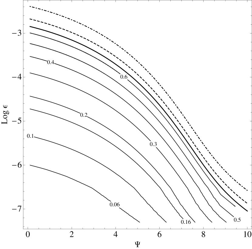
Figure 1.— Parameter space for second-order models. The uppermost solid line represents the critical values of the tidal strength parameter for models in which the potential of the hosting galaxy is Keplerian ($\nu=3$); thin solid lines represent contour levels of the extension parameter $\delta$. The dashed line is the critical curve for models within a logarithmic potential ($\nu=2$). The dot-dashed line gives the critical condition for a potential with $\nu=1$ (e.g., that of a Plummer sphere evaluated at $R_{0}=b/\sqrt{2}$, with $b$ the model scale radius).

2. The Parameter Space

The triaxial tidal models are characterized by two physical scales (corresponding to the two free constants $A$ and $a$ in the distribution function $f_{K}(H)$) and two dimensionless parameters. The latter parameters are best introduced by referring to the formulation of the Poisson equation in terms of the dimensionless escape energy

$$\psi({{\hat{r}}})=a\,H_{0}-[a\,\Phi_{C}({\it\hat{r}})+\epsilon\,T(\hat{x},\hat{z})]~{},$$ (1)

where $a\Phi_{C}$ is the dimensionless cluster mean-field potential (to be determined self-consistently) and $T(\hat{x},\hat{z})=9(\hat{z}^{2}-\nu\hat{x}^{2})/2$ represents the tidal potential (with the numerical coefficient $\nu=4-\kappa^{2}/\Omega^{2}$, where $\kappa$ and $\Omega$ are respectively the epicyclic and orbital frequency, depending on the potential of the hosting galaxy); the hat on the spatial coordinates denotes that they are measured in units of the scale length $r_{0}=[9/(4\pi G\rho_{0}a)]^{1/2}$.

Then the first parameter, already available in the spherical case, is the concentration of the system and can be expressed as a dimensionless measure of the central depth of the potential well: $\Psi\equiv\psi({0})$. The second parameter, the tidal strength $\epsilon$ in Eq. (1), is defined as

$$\epsilon\equiv\frac{\Omega^{2}}{4\pi G\rho_{0}}~{},$$ (2)

i.e. as the ratio of the square of the orbital frequency (of the revolution of the stellar system around the center of the hosting galaxy) to the square of the dynamical frequency associated with the central density $\rho_{0}$ of the stellar system. Alternatively, the effect of the tidal field can be measured by the extension parameter

$$\delta\equiv\hat{r}_{tr}/\hat{r}_{T}~{},$$ (3)

where $\hat{r}_{tr}=\hat{r}_{tr}(\Psi)$ is the truncation radius of the spherical King model characterized by the same value of $\Psi$ and $\hat{r}_{T}$ is the tidal (or Jacobi) radius, i.e. the distance from the origin (the center of the stellar system) of the two nearby Lagrangian points of the restricted three-body problem considered in our simple physical picture. A given model will be labelled by the pair of values $(\Psi,\epsilon)$ or, equivalently, by the pair $(\Psi,\delta)$. The dimensionless cut-off constant $aH_{0}$ can be expressed in a natural way as an asymptotic series with respect to the tidal parameter $aH_{0}=\alpha_{0}+\alpha_{1}\epsilon+\alpha_{2}\epsilon^{2}/2+...$ where the terms $\alpha_{i}$, as discussed in Paper I, depend only on $\Psi$.

Much like the Hill surfaces for the standard restricted three-body problem, we now consider the family of zero-velocity surfaces defined by the condition $\psi({\hat{r}})=0$, which represents the boundary of our models. These surfaces can be open or closed, depending on the value of the cut-off constant $aH_{0}$, which is determined by the selected values of the two dimensionless parameters that characterize the model. To be consistent with the hypothesis of stationarity, we only consider closed configurations. We call “critical models” those that are bounded by the critical zero-velocity surface (which is the outermost available closed surface). For each value of $\Psi$, the critical value of the tidal parameter can be found by (numerically) solving the system

$$\left\{\begin{array}[]{ll}\partial_{\hat{x}}\psi(\hat{x}=\hat{r}_{T},\hat{y}=0,\hat{z}=0;\epsilon_{cr})=0\vspace{.1cm}\\ \psi(\hat{x}=\hat{r}_{T},\hat{y}=0,\hat{z}=0;\epsilon_{cr})=0~{},\end{array}\right.$$ (4)

where the unknowns are $\hat{r}_{T}$ and $\epsilon_{cr}$. The method of matched asymptotic expansions proposed in Paper I for the solution of the relevant Poisson-Laplace equation requires an expansion in spherical harmonics, therefore it can be easily recognized that the first condition of Eq. (4) is equivalent to the requirement of vanishing gradient, which identifies the saddle points of the critical surface. In the general case, the condition $\partial_{\hat{x}}\psi(\hat{r}_{T},0,0;\epsilon)=0$ determines the value of $\hat{r}_{T}$ for a given tidal strength $\epsilon$ , therefore $\hat{r}_{T}=\hat{r}_{T}(\Psi,\epsilon)$.

By using in the escape energy defined in Eq. (1) the zeroth-order expression for the cluster potential $(a\Phi_{C}^{\mbox{\tiny(ext)}})^{(0)}(\hat{r})=\lambda_{0}/\hat{r}$ and for the cut-off constant, the system in Eq. (4) becomes

$$\left\{\begin{array}[]{ll}\displaystyle\frac{\lambda_{0}}{\hat{r}_{T}^{2}}+9\,\epsilon_{cr}\,\nu\hat{r}_{T}=0\vspace{.1cm}\\ \displaystyle\alpha_{0}-\frac{\lambda_{0}}{\hat{r}_{T}}+\frac{9}{2}\,\epsilon_{cr}\,\nu\hat{r}_{T}^{2}=0~{},\end{array}\right.$$ (5)

thus leading to an expression for $\hat{r}_{T}^{(0)}$ in terms of the dimensionless truncation radius of the corresponding spherical King model and a first estimate of the critical value of $\epsilon$

$$\hat{r}_{T}^{(0)}=\frac{3}{2}\frac{\lambda_{0}}{\alpha_{0}}=\frac{3}{2}\hat{r}_{tr}~{},$$ (6)

$$\epsilon_{cr}^{(0)}=-\frac{8\alpha_{0}^{3}}{243\,\nu\,\lambda_{0}^{2}}=-\frac{8}{243\,\nu}\frac{1}{\hat{r}_{tr}^{3}}\lambda_{0}~{}.$$ (7)

The first expression can also be written as $\delta_{cr}^{(0)}=2/3$ (see Spitzer 1987). We recall that $\lambda_{0}=\lambda_{0}(\hat{r}_{tr})$ and that $\hat{r}_{tr}=\hat{r}_{tr}(\Psi)$. Therefore, the right-hand side of Eqs. (6) and (7) depends only on the value of $\Psi$.

Figure 2.— Critical values of the extension parameter for first-order models (dotted) and second-order models (solid) with different potentials of the hosting galaxy ($\nu=3,2,1$ from top to bottom). The dashed horizontal line shows the value 2/3 that is found when a zeroth-order approximation for $a\Phi_{C}$ is used (see Eq. (6)).

Here one important comment is in order. Strictly speaking, the complete solution for $a\Phi_{C}$ derived by the method of matched asymptotic expansions in § 4 of Paper I is a well-justified global uniform solution only for sub-critical (underfilled) models. Close to the condition of criticality, i.e., when $\hat{r}_{tr}\sim\hat{r}_{T}$, in the vicinity of the boundary surface the tidal term $\epsilon\,T$ (which is considered a small correction in the construction of the asymptotic solution) becomes comparable to the cluster term $a\Phi_{C}$, so that the asymptotic solution is expected to break down. For such models, the iteration method described in § 5.2 of Paper I, which does not rely on the assumption that the tidal term is small, is preferred and expected to lead quickly to more accurate solutions. In practice, in line with previous work on the similar problem for rotating polytropes mentioned in the Introduction, we argue that the use of the second-order asymptotic solution constructed in Paper I will give sufficiently accurate solutions in the determination of the critical value of the tidal parameter $\epsilon_{cr}$ from the system in Eq. (4) and in the consequent assessment of the general properties of models even when close to the critical case. The main reason at the basis of this argument is that, even for close-to-critical models, only very few stars populate the region where the asymptotic analysis breaks down, so that the overall solution should be only little affected. A direct comparison between selected critical models calculated with both the perturbation and the iteration method is presented in Appendix A.

If we make use of the full second-order asymptotic solution for the escape energy $\left(\psi^{\mbox{\tiny(ext)}}\right)^{(2)}$, in which the second-order expressions for the cluster potential (recorded in Eq. (B3)) and the cut-off constant are used, the system in Eq. (4) can be re-arranged and written in standard form

$$\left\{\begin{array}[]{ll}A(\hat{r}_{T})\epsilon_{cr}^{2}+2\,B(\hat{r}_{T})\epsilon_{cr}+C(\hat{r}_{T})=0\vspace{.1cm}\\ D(\hat{r}_{T})\epsilon_{cr}^{2}+2\,E(\hat{r}_{T})\epsilon_{cr}+F(\hat{r}_{T})=0~{},\end{array}\right.$$ (8)

with

$$\displaystyle A(\hat{r}_{T})=\lambda_{2}\hat{r}_{T}^{4}-(b_{20}-b_{22}\sqrt{3})\frac{3}{4}\sqrt{\frac{5}{\pi}}\hat{r}_{T}^{2}+b_{40}\frac{45}{16\sqrt{\pi}}$$

$$\displaystyle-b_{42}\frac{15}{8}\sqrt{\frac{5}{\pi}}+b_{44}\frac{15}{16}\sqrt{\frac{35}{\pi}}~{},$$ (9)

$$B(\hat{r}_{T})=\lambda_{1}\hat{r}_{T}^{4}-(a_{20}-a_{22}\sqrt{3})\frac{3}{4}\sqrt{\frac{5}{\pi}}\hat{r}_{T}^{2}+9\nu\hat{r}_{T}^{7}~{},$$ (10)

$$C(\hat{r}_{T})=2\lambda_{0}\hat{r}_{T}^{4}~{},$$ (11)

$$\displaystyle D(\hat{r}_{T})=\alpha_{2}\hat{r}_{T}^{5}-\lambda_{2}\hat{r}_{T}^{4}+(b_{20}-b_{22}\sqrt{3})\frac{1}{4}\sqrt{\frac{5}{\pi}}\hat{r}_{T}^{2}$$

$$\displaystyle-b_{40}\frac{9}{16\sqrt{\pi}}+b_{42}\frac{3}{8}\sqrt{\frac{5}{\pi}}-b_{44}\frac{3}{16}\sqrt{\frac{35}{\pi}}~{},$$ (12)

$$E(\hat{r}_{T})=\alpha_{1}\hat{r}_{T}^{5}-\lambda_{1}\hat{r}_{T}^{4}+(a_{20}-a_{22}\sqrt{3})\frac{1}{4}\sqrt{\frac{5}{\pi}}\hat{r}_{T}^{2}+\frac{9}{2}\nu\hat{r}_{T}^{7}~{},$$ (13)

$$F(\hat{r}_{T})=2(\alpha_{0}\hat{r}_{T}^{5}-\lambda_{0}\hat{r}_{T}^{4})~{},$$ (14)

where the relevant constants ($\lambda_{i}$ with $i=0,1,2$, $a_{lm}$ with $l=0,2$ and $b_{lm}$ with $l=0,2,4$ $m=0,2,...,l$), which are determined by the matching process, are defined in § 4.4 of Paper I. [The corresponding system based on the first-order solution for $\psi^{\mbox{\tiny(ext)}}$ can be recovered by setting $A(\hat{r}_{T})=D(\hat{r}_{T})=0$.] This system has been solved numerically, by means of the Newton-Raphson method, since the equations are nonlinear in $\hat{r}_{T}$ (in particular, they are polynomials of fifth and seventh-order, for the first and second-order solution respectively). As noted in the discussion of the simpler Eq. (5), the solution for $\epsilon_{cr}$ can then be represented as a function of the concentration parameter $\Psi$. The parameter space of the first and second-order models has been explored by means of an equally spaced grid from $\epsilon=5\times 10^{-8}$ to $\epsilon=1\times 10^{-2}$ at steps of $5\times 10^{-7}$ and from $\Psi=0.1$ to $\Psi=10$ at steps of $0.1$.

The parameter space for the second-order models is presented in Fig. 1. The plot provides the contour levels of the extension parameter $\delta$, with the uppermost solid line corresponding to $\delta=\delta_{cr}\approx 2/3$ (thus identifying the critical models), based on the choice $\nu=3$ (Keplerian host galaxy). The critical curves for $\nu=2$ (host galaxy characterized by flat rotation curve) and for $\nu=1$ (Plummer potential evaluated at $R_{0}=b/\sqrt{2}$, with $b$ the model scale radius) are shown as a dashed and dot-dashed line, respectively.

Sub-critical, underfilled models (bottom-left corner of the figure), with $\delta\ll\delta_{cr}$, are only little affected by the tidal perturbation. The maximally deformed models are those with $\delta\approx\delta_{cr}$ (close to the uppermost solid line, i.e. close-to-critical configurations). Figure 1 shows that the critical value for the tidal strength parameter depends strongly on concentration, with a variation of almost four orders of magnitude in the explored range of $\Psi$. The figure also indicates that for lower values of $\nu$ the critical curve moves upwards, i.e. the available parameter space increases.

The difference between the critical value of the tidal strength parameter for first and second-order models (for a chosen value of $\nu$) is very small, around $10^{-5}$ for low-concentration models, down to $10^{-9}$ or less for models with $\Psi\approx 10$. The critical value of the extension parameter $\delta$ depends only weakly on concentration and on $\nu$, as illustrated in Fig. 2.

In closing this section, se should reiterate that, in spite of the abundant use of symbols required by the analysis, the family of models that we have studied is characterized by two dimensionless parameters $(\Psi,\epsilon)$. [As an alternative pair, we may refer to the standard concentration parameter $C=log(r_{tr}/r_{0})$, equivalent to $\Psi$ and frequently used in the context of spherical King models, and to the extension parameter $\delta=\hat{r}_{tr}/\hat{r}_{T}$, equivalent to $\epsilon$.] The free constants $A$ and $a$ that appear in the distribution function $f_{K}(H)$ set the two physical scales. In turn, the models constructed by Heggie & Ramamani (1995) are a one-parameter family of models, because these authors focused on the critical case and did not discuss the sub-critical regime.

Figure 3.— Intrinsic density profiles (normalized to the central value) for critical second-order models with $\nu=3$ and $\Psi=1,2,...,10$ (from left to right). Top panel (a): profile of the triaxial models along the $\hat{x}$-axis (solid) and of the corresponding spherical King models (dashed). Bottom panel (b): profile of the triaxial models along the $\hat{y}$-axis (solid) and the $\hat{z}$-axis (dashed).

3. Intrinsic and projected density distribution

3.1. Intrinsic density profile

The models are characterized by reflection symmetry with respect to the three natural coordinate planes. With respect to the unperturbed configuration (i.e. the spherical King model with the same value of $\Psi$), they exhibit an elongation along the $\hat{x}$-axis (defined by the direction of the center of the host galaxy), a compression along the $\hat{z}$-axis (the direction perpendicular to the orbit plane of the globular cluster), and only a very modest compression along the $\hat{y}$-axis.

Models with $\delta\leq 0.2$, regardless of the value of $\Psi$, are practically indistinguishable from the corresponding spherical King models; significant departures from spherical symmetry occur for models with $\delta\approx 0.4$ or higher. In Fig. 3.a we show the density profile along the $\hat{x}$-axis for a selection of critical second-order models with $\nu=3$ in comparison with that of the corresponding spherical King models; note that for a model with $\Psi=2$ the elongation is already significant at $Log(\rho/\rho_{0})\approx-4$, while for a model with $\Psi=8$ a similar elongation is reached only at much lower density levels ($Log(\rho/\rho_{0})\approx-7$). The corresponding profiles along the $\hat{y}$-axis and the $\hat{z}$-axis are given in Fig. 3.b.

For completeness, we checked the dependence of our density profiles on the potential of the host galaxy. Consistent with the general trends suggested by Fig. 2, the elongation along the $\hat{x}$-axis and the compression along the $\hat{z}$-axis for the models with $\nu=3$ turn out to be slightly weaker than for the models with smaller values of $\nu$.

Figure 4.— Central values of the polar ($e_{0}$; dashed) and equatorial ($\eta_{0}$; solid) eccentricities of the isodensity surfaces of second-order models with $\nu=3$, $\Psi=1,3,5,7$ (from top to bottom) and $\epsilon\in[0,\epsilon_{cr}(\Psi)]$. Horizontal lines mark the maximum value of $e_{0}$ and $\eta_{0}$ reached by the critical models (i.e., for $\epsilon=\epsilon_{cr}(\Psi)$).

Since the dimensionless density distribution of a model, identified by $(\Psi,\epsilon)$, is given by $\hat{\rho}=\hat{\rho}[\psi({\hat{r}})]$, where $\psi$ is the dimensionless escape energy and $\hat{\rho}$ is a monotonically increasing function that vanishes for vanishing argument (see Eq. (11) in Paper I), there is a one-to-one correspondence between isodensity and isovelocity surfaces, the latter being defined by the condition $\psi^{(int)}({\hat{r}})=S$, where $S$ is a constant (with $0\leq S\leq\Psi$). We recall that nonspherical models often exhibit equipotential surfaces rounder than the isodensity surfaces (e.g., see Evans 1993; Ciotti & Bertin 2005). The reason for the presence of this property in our models is that the supporting distribution function depends only on the Jacobi integral, i.e. the (isolating) energy integral in the rotating frame. Therefore, for each value of $S$, we can define the semi-axes $\hat{a}$, $\hat{b}$, and $\hat{c}$ of the corresponding triaxial isodensity surface, by means of the intersections of the surface with the $\hat{x}$, $\hat{y}$, and $\hat{z}$ axes, which turn out to follow the ordering $\hat{a}\geq\hat{b}\geq\hat{c}$. The shape of the triaxial configuration can thus be described in terms of the polar and equatorial eccentricities, defined as $e=[1-(\hat{c}/\hat{a})^{2}]^{1/2}$ and $\eta=[1-(\hat{b}/\hat{a})^{2}]^{1/2}$, respectively.

A surprising result can be derived analytically. In the innermost region $\hat{r}\ll\hat{r}_{tr}$ (i.e., for $S\sim\Psi$), the dimensionless escape energy can be expanded to second order in the dimensionless radius

$$\displaystyle\psi^{(int)}({\bf\hat{r}})\sim\Psi-\frac{3}{2}\hat{r}^{2}+\epsilon\hat{r}^{2}\left[-\frac{3}{2}(1-\nu)+A_{20}Y_{20}(\theta,\phi)+\right.$$ (15)

$$\displaystyle\left.A_{22}Y_{22}(\theta,\phi)\right]+\frac{\epsilon^{2}}{2}\hat{r}^{2}\left[(1+B_{20})Y_{20}(\theta,\phi)+(1+B_{22})Y_{22}(\theta,\phi)\right]~{}.$$

Here some terms of the second-order solution do not contribute (e.g., it can be readily checked that $\psi_{2,4m}^{(int)}(\hat{r})\sim\hat{r}^{4}$ and $\psi_{2,00}^{(int)}(\hat{r})\sim\hat{r}^{6}$). Then by setting $\psi^{(int)}(\hat{a},0,0)=\psi^{(int)}(0,\hat{b},0)=\psi^{(int)}(0,0,\hat{c})$, we find that in the innermost region the eccentricities tend to the following non-vanishing central values

$$e_{0}=\frac{\{\epsilon(A_{22}-\sqrt{3}A_{20}+(\epsilon/2)[1+B_{22}-\sqrt{3}(1+B_{20})])\sqrt{15/\pi}\}^{1/2}}{\{6+2\epsilon[3(1-\nu)-A_{20}\sqrt{5/\pi}]-\epsilon^{2}(1+B_{20})\sqrt{5/\pi}\}^{1/2}}~{},$$ (16)

$$\eta_{0}=\frac{\{\epsilon[2A_{22}+(1+B_{22})\epsilon]\sqrt{15/\pi}\}^{1/2}}{\{6+\epsilon d_{1}+(\epsilon^{2}/2)d_{2}\}^{1/2}}~{},$$ (17)

where

$$d_{1}=6(1-\nu)+(A_{20}+\sqrt{3}A_{22})\sqrt{5/\pi}$$ (18)

$$d_{2}=[1+B_{20}+\sqrt{3}(1+B_{22})]\sqrt{5/\pi}$$ (19)

which depend explicitly on the tidal strength and implicitly on the concentration. This result is nontrivial. In fact, since the tidal potential is a homogeneous function of the spatial coordinates, naively we might expect that in their central region the models reduce to a perfectly spherical shape (i.e., $e_{0}=\eta_{0}=0$), even for finite values of the tidal strength. Instead, $e_{0}$ and $\eta_{0}$ are $\mathcal{O}(\epsilon^{1/2})$ and strictly vanish only in the limit of vanishing tidal strength.

Figure 5.— Profiles of the polar ($e$; dashed) and equatorial ($\eta$; solid) eccentricities of the isodensity surfaces for selected critical second-order models with $\nu=3$ and $\Psi=1,3,5,7$ (from left to right). Dotted horizontal lines show the central eccentricity values (see Eqs. (16) and (17)).

Figure 4 shows the central values of the eccentricities for second-order models with $\nu=3$ and selected values of concentration, as a function of tidal strength within the range $[0,\epsilon_{cr}(\Psi)]$. Consistent with the general trends identified in the discussion of the parameter space, low-concentration models show the most significant departures from spherical symmetry. The full eccentricity profiles (as a function of the major axis) are shown in Fig. 5 for a selection of critical second-order models; here the calculation of $e$ and $\eta$ has been performed by numerically determining the values of the semi-axes of a number of reference isovelocity surfaces, defined by $\psi^{(int)}({\hat{r}})=S_{i}=(25-i)\Psi/25-0.01$ with $i=0,..,25$. Outside the central region, the profiles increase monotonically and, independently of concentration, at the boundary they reach approximately a fixed maximum value ($e\approx 0.78$ and $\eta\approx 0.74$), which corresponds to the fact that the shape of the boundary surface of a critical model ($\delta_{cr}^{(0)}=2/3$; see also Fig. 2) depends only modestly on concentration.

3.2. Comparison with the models constructed by Heggie & Ramamani (1995)

The method used in Paper I for the construction of the models illustrated in this paper can be summarized as follows. The solution in the internal (Poisson) and external (Laplace) domains are expressed as an asymptotic series with respect to the dimensionless parameter $\epsilon$, representing the tidal strength (defined in Eq. (2)), which is considered to be small. The $k$th-order term of the asymptotic series of the internal and external solution are denoted by $\psi_{k}^{\mbox{\tiny(int)}}({\hat{r}})$ and $\psi_{k}^{\mbox{\tiny(ext)}}({\hat{r}})$ respectively, so that the zeroth-order terms define the standard spherical King models (see § 4.1 in Paper I for a detailed discussion). The quantity $(\psi^{\mbox{\tiny(ext)}})^{(k)}$ indicates the $k$th-order external solution, i.e. the corresponding asymptotic series truncated at the term $\psi^{\mbox{\tiny(ext)}}_{k}$; a similar notation holds for the internal solution. The validity of the expansion breaks down where the second term is comparable to the first, i.e. where $\psi_{0}=\mathcal{O}(\epsilon)$. This singularity is cured by introducing a boundary layer in which both the spatial coordinates and the solution $\psi^{\mbox{\tiny(lay)}}$ are suitably rescaled with respect to the tidal parameter. To obtain a uniformly valid solution over the entire space, an asymptotic matching (see Van Dyke 1975; Eq. (5.24)) is performed between the pairs $(\psi^{\mbox{\tiny(int)}},\psi^{\mbox{\tiny(lay)}})$ and $(\psi^{\mbox{\tiny(lay)}},\psi^{\mbox{\tiny(ext)}})$. Each term $\psi_{k}({\hat{r}})$ is then expanded in spherical harmonics with radial coefficients $\psi_{k,\,lm}(\hat{r})$. The internal region requires a numerical solution of the Cauchy problems for the radial coefficients (we used a fourth-order Runge-Kutta code) while in the external region a formal solution with multipolar structure is available and in the boundary layer the integration in the radial variable can be performed analytically (see § 4.2 and 4.3 in Paper I, respectively).

Figure 6.— Relative difference between the intrinsic density profiles of critical second-order models ($\rho_{II}$) constructed in this paper and those of the corresponding (first-order) models ($\rho_{HR}$) described by Heggie & Ramamani (1995). The comparison has been performed along the three axes in the whole internal+boundary region (see main text). Here we illustrate the difference along the $x$-axis in the boundary layer ($\Psi=1,2,...,10$ from left to right). At variance with Fig. 3, the spatial coordinate is scaled with respect to the truncation radius instead of the scale radius $r_{0}$.

The models described by Heggie & Ramamani (1995) are also based on a perturbation approach, but the method used is different from ours, provides a solution of the Poisson equation that is first-order with respect to the tidal parameter, and is restricted to the “critical” case; actually, as noted in § 2 after Eq. (7), the perturbation approach is bound to break down in the critical case. Technically speaking, their method is in the form of a “patching” procedure, in contrast with our asymptotic matching. Therefore, the models constructed in Paper I, while consistent, to first order, with those of Heggie & Ramamani (1995), are more general. We also recall that our method is also applicable to systems described by different distribution functions (see Appendix B and C in Paper I).

We have thus performed a quantitative comparison between the intrinsic density profiles of our critical second-order models and those of the models by Heggie & Ramamani (1995), both referred to the case in which the host galaxy is Keplerian ($\nu=3$). As desired, there is substantial consistency except for the outermost part of the boundary layer in which our models are slightly more compact, due to a global “boxiness” effect induced by the second-order term present in our models in which harmonics of order $l=4$ also play a role. In Fig. 6 we represent the relative difference between the two density profiles evaluated along the $x$-axis (with the coordinates scaled with respect to the truncation radius instead of the usual scale radius $r_{0}$) for selected values of $\Psi$. A similar behaviour is found also along the $y$-axis, for $y/r_{tr}$ in the range $[0.80,1]$, and along the $z$-axis, for $z/r_{tr}$ in the range $[0.80,0.95]$. In the central part of the internal region, along the principal axes, the relative difference is smaller than 5 percent for every value of $\Psi$ we tested, while near the transition to the boundary layer (i.e $x/r_{tr}\lesssim 1$ and $y/r_{tr},\,z/r_{tr}\lesssim 0.8$) a difference of 20 percent can be reached in the case of highly concentrated models ($\Psi=8,9,10$). We interpret these differences as due to the combined effects of the patching vs. matching adopted process and of the different grid on which the Cauchy problems for the radial coefficients are solved (we used a regular radial grid while Heggie & Ramamani (1995) used a more complex tabulation resulting from their choice of taking the zeroth-order cluster potential as the independent variable and of the function $ln(1+\hat{r}^{2})$ instead of $\hat{r}$).

Figure 7.— Ratio of two pairs of quadrupole moments for the second-order models with $\Psi=5$, $0.1\leq\delta\leq\delta_{cr}(\Psi)$, and $\nu=1,2,3$ (in the left panel, the sequence of models with different $\nu$ values runs from bottom to top; in the right panel, it runs from top to bottom). The values obtained from numerical integration over the entire triaxial volume (dots) are compared to the analytical approximations (solid line) given by Eqs. (26) and (25); the analytical estimates of the ratios for first order models are also shown (dashed horizontal lines). The propagation of the errors of the numerical integration leads to the plotted error bars.

3.3. Global quantities

The previous discussion has focused on the shape of the isodensity surfaces of the models. In particular, some interesting conclusions have been derived based on a local analysis of the central region and of the outer boundary of the configuration. The maximal departures from spherical symmetry are reached at the periphery, but these hinge on the distribution of the very small number of stars that populate the outer region of the cluster. We may thus wish to study some global quantities that better characterize whether significant amounts of mass (and, correspondingly, of light) are actually involved in the deviation of the model from spherical symmetry. One standard such global measure is provided by the quadrupole moment tensor

$$\displaystyle Q_{ij}=\int_{V}\,(3x_{i}x_{j}-r^{2}\delta_{ij})\rho({\bf r})d^{3}r=$$

$$\displaystyle\hat{A}r_{0}^{5}\int_{V}\,(3\hat{x}_{i}\hat{x}_{j}-\hat{r}^{2}\delta_{ij})\hat{\rho}({\bf\hat{r}})d^{3}\hat{r}=\hat{A}r_{0}^{5}\hat{Q}_{ij}~{},$$ (20)

with the integration to be performed in the volume $V$ of the entire configuration. Here the notation for the function $\hat{\rho}$ and for the constant $\hat{A}$ is the same as in Eq. (11) of Paper I. In contrast with the frequently used inertia tensor $I_{ij}=\int_{V}\rho x_{i}x_{j}d^{3}r$ (e.g., see Chandrasekhar 1969; chap. 2), the quadrupole moment is defined in such a way that in the spherical limit it vanishes identically. In our coordinate system it is diagonal. Note that the tidal distortions require that the non-vanishing terms of the inertia tensor follow the ordering $I_{xx}\geq I_{yy}\geq I_{zz}$; to visualize the geometry of the system, we may thus also refer to the average polar and equatorial eccentricities $\bar{e}$ and $\bar{\eta}$ defined by the relations $I_{yy}=(1-{\bar{\eta}}^{2})I_{xx}$, $I_{zz}=(1-{\bar{e}}^{2})I_{xx}$. In general, we have $Q_{yy}/Q_{xx}=({\bar{e}}^{2}-2{\bar{\eta}}^{2})/({\bar{e}}^{2}+{\bar{\eta}}^{2})$ and $Q_{zz}/Q_{xx}=({\bar{\eta}}^{2}-2{\bar{e}}^{2})/({\bar{e}}^{2}+{\bar{\eta}}^{2})$, with the prolate configuration identified by ${\bar{e}}={\bar{\eta}}$, i.e. $Q_{yy}/Q_{xx}=Q_{zz}/Q_{xx}=-1/2$.

Since most of the mass is contained in the inner regions, global quantities can be evaluated approximately by neglecting the contribution from the region corresponding to the boundary layer. We can thus use the second-order solutions for $\rho$ obtained in Paper I by the method of matched asymptotic expansions and conveniently reduce the calculation of global quantities to an easier integration in spherical coordinates inside the sphere of radius $\hat{r}_{tr}$. Therefore, for the quadrupole moment tensor we find

$$\hat{Q}_{ij}^{(2)}=\hat{Q}_{ij,1}\epsilon+\hat{Q}_{ij,2}\frac{\epsilon^{2}}{2}~{}.$$ (21)

We emphasize that this estimate is expected to be a good approximation only for those models for which the contribution of the boundary layer is negligible with respect to the one of the internal sphere of radius $\hat{r}_{tr}$.

The relevant components on the diagonal can be expressed in terms of the matching constants of the external solution (for the relevant definitions, see Eqs. (63) and (69) in Paper I)

$$\displaystyle\hat{Q}_{xx}^{(2)}=\frac{2}{9}\sqrt{5\pi}\hat{\rho}(\Psi)\left[\left(a_{20}\epsilon+b_{20}\frac{\epsilon^{2}}{2}\right)\right.$$

$$\displaystyle\left.-\sqrt{3}\left(a_{22}\epsilon+b_{22}\frac{\epsilon^{2}}{2}\right)\right]~{},$$ (22)

$$\displaystyle\hat{Q}_{yy}^{(2)}=\frac{2}{9}\sqrt{5\pi}\hat{\rho}(\Psi)\left[\left(a_{20}\epsilon+b_{20}\frac{\epsilon^{2}}{2}\right)\right.$$

$$\displaystyle\left.+\sqrt{3}\left(a_{22}\epsilon+b_{22}\frac{\epsilon^{2}}{2}\right)\right]~{},$$ (23)

$$\hat{Q}_{zz}^{(2)}=-\frac{4}{9}\sqrt{5\pi}\hat{\rho}(\Psi)\left(a_{20}\epsilon+b_{20}\frac{\epsilon^{2}}{2}\right)~{}.$$ (24)

We recall that the constants $a_{20}$ and $b_{20}$ are positive, while $a_{22}$ and $b_{22}$ are negative (and larger in magnitude). Therefore, $\hat{Q}_{xx}^{(2)}$ is positive and $\hat{Q}_{yy}^{(2)}$ and $\hat{Q}_{zz}^{(2)}$ are negative, consistent with the detailed elongation and compressions observed in the density profile. A summary of the derivation of these formulae is provided in Appendix B.

As a measure of the degree of triaxiality of a given configuration, we have calculated the following ratios

$$\frac{\hat{Q}_{yy}^{(2)}}{\hat{Q}_{xx}^{(2)}}=\frac{\left(a_{20}+b_{20}\epsilon/2\right)+\sqrt{3}\left(a_{22}+b_{22}\epsilon/2\right)}{\left(a_{20}+b_{20}\epsilon/2\right)-\sqrt{3}\left(a_{22}+b_{22}\epsilon/2\right)}~{},$$ (25)

$$\frac{\hat{Q}_{zz}^{(2)}}{\hat{Q}_{xx}^{(2)}}=\frac{-2\left(a_{20}+b_{20}\epsilon/2\right)}{\left(a_{20}+b_{20}\epsilon/2\right)-\sqrt{3}\left(a_{22}+b_{22}\epsilon/2\right)}~{},$$ (26)

which depend explicitly on the tidal strength parameter and implicitly on the concentration parameter. In the limit of vanishing tidal strength, we find

$$\frac{\hat{Q}_{yy}}{\hat{Q}_{xx}}\sim\frac{\hat{Q}_{yy}^{(1)}}{\hat{Q}_{xx}^{(1)}}=\frac{T_{20}(\hat{r}_{tr})+\sqrt{3}T_{22}(\hat{r}_{tr})}{T_{20}(\hat{r}_{tr})-\sqrt{3}T_{22}(\hat{r}_{tr})}=-\frac{\nu-1}{2\nu+1}~{},$$ (27)

$$\frac{\hat{Q}_{zz}}{\hat{Q}_{xx}}\sim\frac{\hat{Q}_{zz}^{(1)}}{\hat{Q}_{xx}^{(1)}}=\frac{-2T_{20}(\hat{r}_{tr})}{T_{20}(\hat{r}_{tr})-\sqrt{3}T_{22}(\hat{r}_{tr})}=-\frac{2+\nu}{2\nu+1}~{},$$ (28)

where $T_{2m}(\hat{r})$ are the quadrupole coefficients of the tidal potential (see Eqs. (38) and (39) in Paper I). This result is nontrivial, because, in this limit, numerator and denominator are both expected to vanish. Note that only for $\nu=1$ the ratio ${\hat{Q}_{yy}}/{\hat{Q}_{xx}}=\mathcal{O}(\epsilon)$.

Earlier in this paper we mentioned that two physical scales, such as total mass and central velocity dispersion, correspond to the two dimensional constants $A$ and $a$ that appear in the distribution function $f_{K}(H)$. In fact, the total mass of the system is given by

$$M=\int_{V}\,\rho({r})d^{3}r=\hat{A}r_{0}^{3}\int_{V}\,\hat{\rho}({\hat{r}})d^{3}\hat{r}=\hat{A}r_{0}^{3}\hat{M}~{}.$$ (29)

If we insert the second-order solution for $\rho$ obtained in Paper I, we find

$$\displaystyle\hat{M}^{(2)}=\int_{0}^{2\pi}d\phi\int_{0}^{\pi}d\theta\sin\theta\int_{0}^{\hat{r}_{tr}}d\hat{r}\,\hat{r}^{2}\,\hat{\rho}^{(2)}(\hat{r},\theta,\phi)$$

$$\displaystyle=\hat{M}_{0}+\epsilon\hat{M}_{1}+\frac{\epsilon^{2}}{2}\hat{M}_{2}~{},$$ (30)

with

$$\hat{M}_{i}=\hat{M}_{i}(\Psi)=-\frac{4\pi\hat{\rho}(\Psi)}{9}\lambda_{i}~{}.$$ (31)

Here each term of the expansion is related to the corresponding constant with $l=0$ (i.e., the monopole term) of the expression of the external solution of the Poisson-Laplace equation calculated by means of the method of matched asymptotic expansion (for the relevant definitions, see Eqs. (59),(61),(67) in Paper I).

The quality of the analytical estimates for the total mass and the quadrupole moment tensor has been checked by comparing the values obtained from asymptotic analysis with those resulting from direct numerical integration of Eq. (29) and Eq. (3.3) respectively, in which the density profile $\hat{\rho}=\hat{\rho}[\psi({\hat{r}})]$ is used without any additional expansion. The integration of the distribution function over the entire space, required by those global quantities, has been performed by means of an Adaptive Monte Carlo method (the algorithm VEGAS, see Press et al. 1992; § 7.8), well suited for our geometry. For the quadrupole, the results are illustrated in Fig. 7. For the mass, the dimensionless function $\hat{M}^{(2)}(\Psi)$ is basically unchanged (within 0.5 percent) with respect to the function characterizing the spherical King models; the Monte Carlo integration is very accurate, with relative errors around $10^{-5}$, and the analytical approximation given by Eq. (3.3) shows an excellent agreement for every value of $\Psi$ in the whole range of the extension parameter $[0,\delta_{cr}(\Psi)]$.

Figure 8.— Average polar ($\bar{e}$; dashed) and equatorial ($\bar{\eta}$; solid) eccentricities for critical second-order models as a function of concentration, with $0.1\leq\Psi\leq 10$, for two different host potentials. Models with $\nu=3$ correspond to the inner pair of curves, while models with $\nu=1$ to the outer pair. The eccentricities have been determined numerically from their definitions (see main text) in terms of $\hat{\rho}=\hat{\rho}[\psi({\bf\hat{r}})]$, without any additional expansion; the relative errors are around $10^{-5}$.

The average eccentricities for critical second-order models as a function of concentration, with $0.1\leq\Psi\leq 10$, for two different choices of the host galaxy potential ($\nu=3,1$), are shown in Fig. 8. The values are calculated directly from the definitions given earlier in this subsection in terms of $\hat{\rho}=\hat{\rho}[\psi({\hat{r}})]$ with no additional expansions. A non-monotonic dependence on concentration is revealed, with generally higher average eccentricities attained by low-concentration models. The trends of the polar and equatorial eccentricities are basically the same, as shown by the fact that the related curves in the plot can be matched approximately by a rigid translation. As expected (see § 3.1), models with $\nu=1$ show a larger separation between polar and equatorial eccentricities than models with $\nu=3$. The presence of a minimum for the curves at $\Psi\approx 6.5$ occurs approximately at the location where the function $Log[\epsilon_{cr}(\Psi)]$ shows an inflection point (regardless of the value of $\nu$; see Fig. 1).

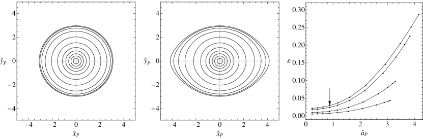
Figure 9.— Projections of a second-order critical model ($\Psi=2$ and $\nu=3$) along the $\hat{x}$ axis (left panel [a]) and along the $\hat{y}$ axis (central panel [b]). The ellipticity profiles (right panel [c], from bottom to top) refer to the projections along directions identified by $(\theta=\pi/2,\phi=i\,\pi/6)$ with $i=0,...,3$; dots represent the locations of the isophotes drawn in panels [a],[b], which correspond to selected values of $\Sigma/\Sigma_{0}$ in the range $[0.9,10^{-6}]$. The arrow indicates the position of the half-light isophote (practically the same for every projection considered in the figure).

3.4. Projected density profile

Under the assumption of a constant mass-to-light ratio, projected models can be compared with the observations. We have then computed surface (projected) density profiles and projected isophotes. The projection has been performed along selected directions, identified by the viewing angle $(\theta,\phi)$, corresponding to the $\hat{z}_{P}$ axis of a new coordinate system related to the intrinsic system by the transformation ${\hat{x}}_{P}=R{\hat{x}}$; the rotation matrix $R=R_{1}(\theta)R_{3}(\phi)$ is expressed in terms of the viewing angles, by taking the $\hat{x}_{P}$ axis as the line of nodes (see Ryden 1991; for an equivalent projection rule). Given the symmetry of our models (see § 3.1), viewing angles can be chosen from the first octant only. In particular, we used a $4\times 4$ polar grid defined by $\theta_{i}=i\,\pi/6$ and $\phi_{j}=j\,\pi/6$ with $i,j=0,..,3$, and calculated (by numerical integration, using the Simpson rule) the dimensionless projected density

$$\hat{\Sigma}(\hat{x}_{P},\hat{y}_{P})=\int_{-\hat{z}_{sp}}^{\hat{z}_{sp}}\hat{\rho}({\hat{r}}_{P})d\hat{z}_{P}~{},$$ (32)

where $\hat{z}_{sp}=(\hat{x}_{e}^{2}-\hat{x}_{P}^{2}-\hat{y}_{P}^{2})^{1/2}$ with $\hat{x}_{e}$ the edge of the cluster along the $\hat{x}$ axis of the intrinsic coordinate system (i.e., we “embedded” the triaxial configuration in a sphere of radius given by its maximal extension). The projection plane $(\hat{x}_{P},\hat{y}_{P})$ has been sampled on an equally-spaced $108\times 108$ square grid centered at the origin (note that for $\hat{x}_{P}^{2}+\hat{y}_{P}^{2}\geq\hat{x}_{e}^{2}$ the projected density is correctly set to zero).

The morphology of the isophotes of a given projected image can be described in terms of the ellipticity profile, defined as $\varepsilon=1-\hat{b}_{P}/\hat{a}_{P}$ where $\hat{a}_{P}$ and $\hat{b}_{P}$ are the semi-axes, as a function of the major axis $\hat{a}_{P}$. As already noted for the (intrinsic) eccentricity profiles, the deviation from circularity increases with the distance from the origin. In the inner region, the ellipticity is consistent with the central eccentricities $e_{0}$ and $\eta_{0}$ calculated in § 3.2.

By taking lines of sight different from the axes of the symmetry planes, we have also checked whether the projected models would exhibit isophotal twisting. For all the cases considered, the position angle of the major axis remains unchanged over the entire projected image. Tests made by changing the resolution of the grid confirm that, even in the most triaxial case ($\nu=1$), no significant twisting is present.

The first two panels of Fig. 9 show the projected images of a critical second-order model with $\Psi=2$ and $\nu=3$ along the $(\pi/2,0)$ and $(\pi/2,\pi/2)$ directions, (i.e., the $\hat{x}$ and $\hat{y}$ axis of the intrinsic system), corresponding, respectively, to the least and to the most favorable line of sight for the detection of the intrinsic flattening of the model. For the same model, the third panel illustrates the ellipticity profiles for various lines of sight.

Figure 10 shows the surface density profiles along the $\hat{x}_{P}$ and $\hat{y}_{P}$ axes of the projection plane for ten critical second-order models with $\nu=3$, viewed along the $(\pi/2,\pi/2)$ direction. As a further characterization, for the same models in the lower panel we also present the surface density profiles obtained by averaging the projected density distribution on circular annuli; this conforms to the procedure often adopted by observers in dealing with density distributions with very small departures from circular symmetry (e.g., see Lanzoni et al. 2007). As expected, circular-averaged profiles lie between the corresponding regular profiles taken along the principal axes of the projected image.

4. Intrinsic and projected kinematics

By construction, the models are characterized by isotropic velocity dispersion. The intrinsic velocity dispersion can be determined directly as the second moment in velocity space (normalized to the intrinsic density) of the distribution function

$$\sigma^{2}(\psi)=\frac{2}{5a}\frac{\gamma\left(7/2,\psi\right)}{\gamma\left(5/2,\psi\right)}=\frac{1}{a}\hat{\sigma}^{2}(\psi)~{},$$ (33)

where $\gamma$ represents the incomplete gamma function (near the boundary of the configuration, the velocity dispersion profile scales as $\hat{\sigma}^{2}(\psi)\sim(2/7)\psi$). This shows that the isodensity surfaces of the models are in a one-to-one correspondence with the isovelocity and isobaric surfaces (defined by $\sigma^{2}[\psi({\hat{r}})]=$ const). As noted for the intrinsic density profiles in § 3.1, a compression along the $\hat{z}$ axis and an elongation along $\hat{x}$ axis occur also for the intrinsic velocity dispersion profiles. In Fig. 11.a we present the intrinsic velocity dispersion profiles along the $\hat{x}$ axis for the same critical models illustrated in Fig. 3 compared to the profiles of the corresponding spherical King models. The behavior of the projected velocity dispersion profiles near the boundary is significantly different from that of the spherical models.

The projected velocity moments can be calculated by integrating along the line of sight (weighted by the intrinsic density) the corresponding intrinsic quantities. Therefore, the projected velocity dispersion is given by

$$\displaystyle\sigma^{2}_{P}(\hat{x}_{P},\hat{y}_{P})=\frac{\int_{-\hat{z}_{sp}}^{\hat{z}_{sp}}\sigma^{2}({\bf\hat{r}}_{P})\rho({\bf\hat{r}}_{P})d\hat{z}_{P}}{\Sigma(\hat{x}_{P},\hat{y}_{P})}=$$

$$\displaystyle\frac{2}{5a}\frac{\int_{-\hat{z}_{sp}}^{\hat{z}_{sp}}\gamma[7/2,\psi({\bf\hat{r}}_{P})]\exp[\psi({\bf\hat{r}}_{P})]d\hat{z}_{P}}{\hat{\Sigma}(\hat{x}_{P},\hat{y}_{P})}=\frac{1}{a}\hat{\sigma}^{2}_{P}(\hat{x}_{P},\hat{y}_{P})~{}.$$ (34)

Figure  11.b shows the projected velocity dispersion profiles along the $\hat{x}_{P}$ and $\hat{y}_{P}$ axis of the projection plane for the same models displayed in Fig. 10 (the line of sight is defined by $(\pi/2,\pi/2)$).

Figure 10.— Projected density profiles (normalized to the central value) for the same ten second-order critical models displayed in Fig. 3. Top panel (a): the models are viewed from the $\hat{y}$ axis and the profiles taken along the two principal axes in the projection plane (along $\hat{x}_{P}$ (solid) and $\hat{y}_{P}$ (dashed), i.e. along the $\hat{x}$ and $\hat{z}$ axes of the intrinsic frame of reference). Bottom panel (b): the projection is performed on the same line of sight of the previous panel, but the profiles are taken by averaging the projected surface density on circular annuli, as if the image were intrinsically circular.

5. Discussions and conclusions

5.1. A comment on the complex structure of the outer regions

In Paper I we have noted the singular character of the mathematical problem associated with the free boundary set by the three-dimensional surface of these tidally truncated models. In § 2 of the present Paper, we have further emphasized the additional singularity that characterizes close-to-critical models (see comment after Eq. (7), which prompted the analysis described in the Appendix A). As is true in general in the study of boundary layers and similar problems, it is no wonder that in the vicinity of such critical boundaries, a number of complex physical effects may take place and play an important role in determining the detailed structure of the solution. On the other hand, the properties of the derived solution away from the boundary are quite robust (see § 3.3 and the Appendix). As to some of the subtle properties of the expected distribution function close to the edge of a cluster, it is interesting to summarize here below the main results that emerge from a vast body of evolutionary models (N-body, Fokker-Planck, Monte Carlo, gas), on the issue of the interplay between pressure anisotropy and tidal effects.

Since the first solutions of the Fokker-Planck equation by means of a Monte Carlo approach, as described by Hénon (1971) or Spitzer & Hart (1971), it has been shown that one-component isolated spherical clusters, starting from a variety of initial conditions (see Spitzer 1987; chap.4 and references therein), develop a core-halo structure in which the central parts are almost isotropic while the outer regions are characterized by radial anisotropy. A commonly reported interpretation is that the halo is mainly populated by stars scattered out from the core on radial orbits. If the evolution of a cluster is influenced not only by internal processes but also by the presence of an external tidal field, the growth of pressure anisotropy is significantly damped. Direct N-body simulations (e.g., see Giersz & Heggie 1997; Aarseth & Heggie 1998; Baumgardt & Makino 2003; Lee et al. 2006), anisotropic Fokker-Planck (e.g., see Takahashi et al. 1997), and Monte Carlo models (e.g., see Giersz 2001) of both single and multi-mass systems suggest that clusters in circular orbits (and even in eccentric orbits, see Baumgardt & Makino 2003), starting from isotropic initial conditions, tend to preserve pressure isotropy, except for the outermost parts which become tangentially anisotropic due to the preferential loss of stars on radial orbits, induced by the tidal field. The overall agreement on this result is nontrivial, because of the aforementioned differences in the treatment of the external tidal field. Even extreme cases of time-dependent tides, such as disk shocking, influence the degree of pressure anisotropy since it has been shown that they may represent a dominant mechanism (“shock relaxation”) of the energy redistribution, leading to a substantial isotropy, of the weakly bound stars (see Oh & Lin 1992; Kundic & Ostriker 1995; both papers are based on a Fokker-Planck approach).

These results confirm that, of course, the properties of the models constructed in Paper I and described in this paper should be taken only as a zeroth-order reference frame, to single out the precise role of external tides, and should not be taken literally as a realistic representation of real objects since a number of simplifying assumptions are made. On the other hand, by comparing data with such an idealized reference model it will be possible to better assess the role of tides with respect to other physical ingredients studied separately.

Figure 11.— Top panel (a): intrinsic velocity dispersion profiles (solid, normalized to the central value) along the $\hat{x}$ axis for the same ten second-order critical models illustrated in Fig. 3.a compared to the corresponding spherical King models (dashed). Bottom panel (b): projected velocity dispersion profiles (normalized to the central value) for the same ten second-order critical models illustrated in Fig. 10.a, viewed along the same direction. Solid and dashed lines show the profiles along the $\hat{x}_{P}$ axis and $\hat{y}_{P}$ of the projection plane, respectively.

5.2. Summary and concluding remarks

The main results that we have obtained from the detailed analysis of the family of tidal triaxial models can be summarized as follows:

1. Two tidal regimes exist, namely of low and high-deformation, which are determined by the combined effect of the tidal strength of the field and of the concentration of the cluster. The degree of deformation increases with the degree of filling of the relevant Roche volume. Far from the condition of Roche volume filling, the models are almost indistinguishable from the corresponding spherical King models. A number of studies have investigated the evolution of tidally perturbed stellar systems initially underfilling their Roche lobe (e.g., see Gieles & Baumgardt 2008; Vesperini et al. 2009), concluding that some of the relevant dynamical processes, in particular evaporation, depend on the degree of filling of the Roche volume. The intrinsic properties of the models discussed in this paper can be useful for setting self-consistent nonspherical initial conditions of numerical simulations aiming at studying in further details the evolution of configurations starting from sub-critical tidal equilibria.

2. For a given tidal strength, there exists a maximum value of concentration for which a closed configuration is allowed (see Fig. 1). In such “critical” case, the truncation radius of the corresponding spherical King models is of the same order of the tidal radius of the triaxial model. The shape of the boundary of the maximally deformed models is given by the “critical” zero-velocity surface of the relevant Jacobi integral and is basically independent of concentration, while the deformation of the internal region strongly depends on the value of the critical tidal strength and is more significant for low-concentration models. This statement agrees with a general trend noted by White & Shawl (1987) for the globular cluster system of our Galaxy.

3. The structure of the models can be described in terms of the polar and equatorial eccentricity profiles of the intrinsic isodensity surfaces. The maximal departures from spherical symmetry are reached in the outskirts.

4. For finite tidal strength, the central values of the polar and equatorial eccentricities are finite, $\mathcal{O}(\epsilon^{1/2})$; this result is nontrivial since the tidal potential which induces the perturbation is a quadratic homogeneous function of the spatial coordinates.

5. Global measures of the degree of triaxiality in terms of the quadrupole moment tensor have been introduced and calculated for different values of the tidal strength and different potentials of the host galaxy. The potential of the host galaxy sets the geometry of the tidal perturbation, as nicely shown by the analytic expressions for the ratios of the components of the quadrupole moment tensor, which, in the case of first-order models, reduce to simple functions of the coefficient $\nu$. Average eccentricities have been calculated from the inertia tensor components, evaluated numerically.

6. As a key step in the direction of a comparison with observations, projected density profiles and ellipticity profiles have been calculated for a number of models for several lines of sight.

7. The study of the relevant (projected) isophotes indicates that no isophotal twisting occurs. This result is nontrivial since the models are nonstratified and centrally-concentrated, conditions under which, in principle, isophotal twist may occur (see Stark (1977); models based on Stäckel potentials are also known to be twist-free, as shown by Franx (1988)).

8. Finally, close to the boundary, the intrinsic and projected kinematics shows significant differences with respect to that of spherical models.

Since our models are all characterized by monotonically increasing ellipticity profiles, they cannot explain the variety of behavior of observed ellipticity profiles (see Geyer et al. 1983), but the range of the predicted flattening ($\varepsilon<0.3$) is consistent with that observed in most globular clusters (see White & Shawl (1987) for the clusters in the Milky Way and Frenk & Fall (1982) for those in the LMC). Therefore, with the exception of special clusters such as Omega Centauri, we think that the modest but frequently observed deviations from spherical symmetry might have their origin traced to tides.

Finally, since our models are intrinsically more elongated (in the direction of the center of the host galaxy) than spherical King models, they might be useful for interpreting clusters with a surface brightness profile extending beyond that predicted by the spherical King models. Recent investigations (see McLaughlin & van der Marel 2005) suggest that such “extra-tidal” structures are a fairly generic feature, especially for extragalactic clusters, and not just a transient property, present only at young ages.

On the basis of the work presented here, in a following paper we plan to address in detail the issues raised by observations.

Appendix A Perturbation vs. iteration

For completeness, we calculated selected models also by means of the iteration method described in § 5.2 of Paper I, in order to verify the quality of the solution obtained with the method of matched asymptotic expansions, in particular in the critical regime. This technique follows the approach proposed by Prendergast & Tomer (1970). The basic idea is to get an improved solution of the Poisson equation (see Eq. (77) in Paper I) by evaluating the right-hand side with the solution obtained from the immediately previous step, starting from the spherical King models taken as initial “seed solutions”. In our code, the required spherical harmonic analysis and synthesis of density and potential have been performed by means of the S2kit 1.0 package (Kostelec & Rockmore 2004), which makes use of FFTW 3.2.1 (Frigo & Johnson 2005). We decided to truncate the harmonic series at $l=4$ in order to be consistent with the maximum harmonic index admitted by the second-order asymptotic solution. The iteration stops when convergence to four significant digits in the whole domain of the solution is reached.

For selected values of the concentration parameter in the range $0.1\leq\Psi\leq 10$ (for simplicity, we considered only the case of an external potential with $\nu=3$), the corresponding critical value of the tidal strength parameter obtained with the iteration method is consistent to $10^{-3}$ with the value determined by the numerical solution of Eq. (8), in which the constants obtained from the asymptotic matching are used. For a critical model up to 20 iteration steps are required for convergence, while a subcritical solution typically takes in 4 to 8 steps.

Appendix B Global quantities from the multipole expansion of the cluster potential

Based on the expansion in spherical harmonics of $1/|{\hat{r}}-{\hat{r}^{\prime}}|$ given in Eq. (3.70) of Jackson (1999), the external potential generated by our model can be expressed by means of the following multipole expansion

$$a\Phi_{C}^{\mbox{\tiny(ext)}}({\hat{r}})=-\frac{9}{4\pi\hat{\rho}(\Psi)}\int_{V}d^{3}\hat{r}^{\prime}\frac{\hat{\rho}({\hat{r}^{\prime}})}{|{\hat{r}}-{\hat{r}^{\prime}}|}=-\frac{9}{\hat{\rho}(\Psi)}\sum_{l=0}^{+\infty}\frac{1}{2l+1}\sum_{m=-l}^{+l}\hat{q}_{lm}\frac{Y_{lm}(\theta,\phi)}{\hat{r}^{l+1}}~{},$$ (B1)

where the multipole coefficients are defined as

$$\hat{q}_{lm}=\int_{V}d^{3}\hat{r}^{\prime}Y_{lm}(\theta^{\prime},\phi^{\prime})\hat{r}^{\prime\,l}\hat{\rho}({\hat{r}^{\prime}})~{},$$ (B2)

with the integration to be performed in the volume $V$ with boundary surface defined by $\psi=0$. This general expression can be compared with the second-order solution of the Laplace equation obtained in Paper I

$$\left(a\Phi_{C}^{\mbox{\tiny(ext)}}\right)^{(2)}({\hat{r}}) = \left[\lambda_{0}+\lambda_{1}\epsilon+\lambda_{2}\frac{\epsilon^{2}}{2}\right]\frac{1}{\hat{r}}+\left[a_{20}\epsilon+b_{20}\frac{\epsilon^{2}}{2}\right]\frac{Y_{20}(\theta,\phi)}{\hat{r}^{3}}+\left[a_{22}\epsilon+b_{22}\frac{\epsilon^{2}}{2}\right]\frac{Y_{22}(\theta,\phi)}{\hat{r}^{3}}$$ (B3)

$$+b_{40}\frac{\epsilon^{2}}{2}\frac{Y_{40}(\theta,\phi)}{\hat{r}^{5}}+b_{42}\frac{\epsilon^{2}}{2}\frac{Y_{42}(\theta,\phi)}{\hat{r}^{5}}+b_{44}\frac{\epsilon^{2}}{2}\frac{Y_{44}(\theta,\phi)}{\hat{r}^{5}}~{},$$

in order to determine the relation between the second-order multipole coefficients $\hat{q}_{lm}^{(2)}$ (i.e. calculated by means of the second-order expression for the density) and the matching constants that appear in Eq. (B3). Therefore, we find that

$$\lambda_{0}+\lambda_{1}\epsilon+\lambda_{2}\frac{\epsilon^{2}}{2}=-\frac{9}{\sqrt{4\pi}\hat{\rho}(\Psi)}\,\hat{q}_{00}^{(2)}~{},$$ (B4)

so that Eq. (31) follows. For the higher-order harmonics we find the following relations for the non-vanishing coefficients

$$a_{2m}\epsilon+b_{2m}\frac{\epsilon^{2}}{2}=-\frac{9}{5\hat{\rho}(\Psi)}\,\hat{q}_{2m}^{(2)}~{},$$ (B5)

for $m=0,2$ and

$$b_{4m}\frac{\epsilon^{2}}{2}=-\frac{1}{\hat{\rho}(\Psi)}\,\hat{q}_{4m}^{(2)}~{},$$ (B6)

for $m=0,2,4$.

Recalling that we are using real spherical harmonics with the Condon-Shortley phase, we get

$$\hat{q}_{20}=\frac{1}{4}\sqrt{\frac{5}{\pi}}\hat{Q}_{zz}~{},$$ (B7)

$$\hat{q}_{22}=\frac{1}{12}\sqrt{\frac{15}{\pi}}(\hat{Q}_{xx}-\hat{Q}_{yy})~{}.$$ (B8)

To determine all the nontrivial components of the quadrupole moment tensor, we use the condition $\mbox{Tr}(\hat{Q}_{ij})=0$. Therefore, for the second-order solution of Paper I, the system

$$\left\{\begin{array}[]{lll}\displaystyle\hat{Q}_{xx}^{(2)}-\hat{Q}_{yy}^{(2)}=-\frac{20}{3}\sqrt{\frac{\pi}{15}}\hat{\rho}(\Psi)\left(a_{22}\epsilon+b_{22}\frac{\epsilon^{2}}{2}\right)\vspace{.1cm}\\ \displaystyle\hat{Q}_{zz}^{(2)}=-\frac{20}{9}\sqrt{\frac{\pi}{5}}\hat{\rho}(\Psi)\left(a_{20}\epsilon+b_{20}\frac{\epsilon^{2}}{2}\right)\vspace{.1cm}\\ \displaystyle\hat{Q}_{xx}^{(2)}+\hat{Q}_{yy}^{(2)}+\hat{Q}_{zz}^{(2)}=0~{},\end{array}\right.$$ (B9)

leads to the expressions recorded in Eqs. (3.3)-(24).

References

- Aarseth & Heggie (1998) Aarseth, S. J., & Heggie, D. C. 1998, MNRAS, 297, 794
- Baumgardt & Makino (2003) Baumgardt, H., & Makino, J. 2003, MNRAS, 340, 227
- Bertin & Varri (2008) Bertin, G., & Varri, A. L., 2008, ApJ, 689, 1005 (Paper I)
- Chandrasekhar (1969) Chandrasekhar, S., 1969, Ellipsoidal Figures of Equilibrium (New Haven, CT: Yale Univ. Press)
- Chernoff & Weinberg (1990) Chernoff, D. F., & Weinberg, M. D. 1990, ApJ, 351, 121
- Ciotti & Bertin (2005) Ciotti, L., & Bertin, G. 2005, A&A, 437, 419
- Einsel & Spurzem (1999) Einsel, C., & Spurzem, R. 1999, MNRAS, 302, 81
- Evans (1993) Evans, N. W. 1993, MNRAS, 260, 191
- Fall & Frenk (1985) Fall, S. M., & Frenk, C. S. 1985, in IAU Symp. 113, Dynamics of Star Clusters, ed. J. Goodman & P. Hut (Dordrecht: Reidel), 285
- Franx (1988) Franx, M. 1988, MNRAS, 231, 285
- Frigo & Johnson (2005) Frigo, M., & Johnson, S. G. 2005, in Proceedings of the IEEE 93, 2, 216
- Frenk & Fall (1982) Frenk, C. S., & Fall, S. M. 1982, MNRAS, 199, 565
- Geyer et al. (1983) Geyer, E. H., Nelles, B., & Hopp, U. 1983, A&A, 125, 359
- Gieles & Baumgardt (2008) Gieles, M., & Baumgardt, H. 2008, MNRAS, 389, L28
- Giersz & Heggie (1997) Giersz, M., & Heggie, D. C. 1997, MNRAS, 286, 709
- Giersz (1998) Giersz, M. 1998, MNRAS, 298, 1239
- Giersz (2001) Giersz, M. 2001, MNRAS, 324, 218
- Han & Ryden (1994) Han, C., & Ryden, B. S. 1994, ApJ, 433, 80
- Heggie & Ramamani (1995) Heggie, D. C., & Ramamani, N. 1995, MNRAS, 272, 317
- Heggie & Hut (2003) Heggie, D., & Hut, P. 2003, The Gravitational Million-Body Problem (Cambridge, UK: Cambridge Univ. Press)
- Hénon (1971) Hénon, M. 1971, Ap&SS, 13, 284
- Jackson (1999) Jackson, J. D. 1999, Classical Electrodynamics (3rd ed.; Hoboken, NJ: John Wiley & Sons)
- Joshi et al. (2000) Joshi, K. J., Rasio, F. A., & Portegies Zwart, S. 2000, ApJ, 540, 969
- King (1961) King, I. R. 1961, AJ, 66, 68
- King (1966) King, I. R. 1966, AJ, 71, 64
- Kostelec & Rockmore (2004) Kostelec, P.J., & Rockmore, D.N. 2004, S2kit: A Lite Version of Spharmonic Kit (Hanover, NH: Darthmouth College, Department of Mathematics), http://www.cs.dartmouth.edu/ geelong/sphere/s2kit_fx.pdf
- Kundic & Ostriker (1995) Kundic, T., & Ostriker, J. P. 1995, ApJ, 438, 702
- Lanzoni et al. (2007) Lanzoni, B., Dalessandro, E., Perina, S., Ferraro, F. R., Rood, R. T., & Sollima, A. 2007, ApJ, 670, 1065
- Lee et al. (2006) Lee, K. H., Lee, H. M., & Sung, H. 2006, MNRAS, 367, 646
- McLaughlin & van der Marel (2005) McLaughlin, D. E., & van der Marel, R. P. 2005, ApJS, 161, 304
- Oh & Lin (1992) Oh, K. S., & Lin, D. N. C. 1992, ApJ, 386, 519
- Portegies Zwart et al. (2001) Portegies Zwart, S. F., McMillan, S. L. W., Hut, P., & Makino, J. 2001, MNRAS, 321, 199
- Prendergast & Tomer (1970) Prendergast, K. H., & Tomer, E. 1970, AJ, 75, 674
- Press et al. (1992) Press W. H., Teukolsky S. A., Vetterling W. T., & Flannery B. P. 1992, Numerical Recipes in Fortran 77 (2nd ed.; UK: Cambridge University Press)
- Ryden (1991) Ryden, B. S. 1991, MNRAS, 253, 743
- Smith (1975) Smith, B. L. 1975, Ap&SS, 35, 223
- Smith (1976) Smith, B. L. 1976, Ap&SS, 43, 411
- Spitzer & Hart (1971) Spitzer, L. J., & Hart, M. H. 1971, ApJ, 166, 483
- Spitzer (1987) Spitzer, L. 1987, Dynamical Evolution of Globular Clusters (Princeton, NJ: Princeton Univ. Press)
- Stark (1977) Stark, A. A. 1977, ApJ, 213, 368
- Takahashi et al. (1997) Takahashi, K., Lee, H. M., & Inagaki, S. 1997, MNRAS, 292, 331
- van den Bergh (2008) van den Bergh, S. 2008, AJ, 135, 1731
- Van Dyke (1975) Van Dyke, M. 1975, Perturbation Methods in Fluid Mechanics (Annotated ed.; Stanford, CA: The Parabolic Press)
- Vesperini et al. (2009) Vesperini, E., McMillan, S. L. W., & Portegies Zwart, S. 2009, ApJ, 698, 615
- Weinberg (1993) Weinberg, M. D. 1993, in ASP Conf. Ser. 48, The Globular Cluster-Galaxy Connection, ed. G. H. Smith, & J. P. Brodie, (San Francisco: ASP), 689
- White & Shawl (1987) White, R. E., & Shawl, S. J. 1987, ApJ, 317, 246