Models of Isospin Breaking in the Pion Form Factor: Consequences for the Determination of $\Pi_{\rho\omega}(m_{\rho}^{2})$ and $(g-2)_{\mu}/2$

Abstract

We study the implications of several recent high-precision measurements of the pion form factor in the region of the $\rho-\omega$ interference “shoulder” for (i) the extraction of the $\rho-\omega$ mixing matrix element, $\Pi_{\rho\omega}(m_{\rho}^{2})$, and (ii) the evaluation of the isospin-breaking (IB) correction needed to incorporate hadronic $\tau$ decay data into the determination of the Standard Model expectation for the leading order hadronic contribution, $[a_{\mu}]_{had}^{LO}$, to the anomalous magnetic moment of the muon, focussing, in the latter case, on the model-dependence of the $\rho-\omega$ mixing component of the IB correction. We consider a range of different models for the broad $\rho$ contribution to the $e^{+}e^{-}\rightarrow\pi\pi$ amplitude, applying these models to each experimental data set, and find that the model dependence of the $\rho-\omega$ mixing correction is significantly larger than the uncertainty induced by experimental errors for any individual model. We also find that, for each such model, the recent data allows one to separate $\rho-\omega$ mixing and direct $\omega\to\pi\pi$ coupling contributions to the amplitude, and hence to obtain a reasonably precise extraction of $\Pi_{\rho\omega}(m_{\rho}^{2})$, uncontaminated by direct $\omega\rightarrow\pi\pi$ coupling effects, for use in meson exchange model calculations of charge symmetry breaking in $NN$ scattering.

I Introduction

The pion form factor, $F_{\pi}(s)$, in the $\rho$ resonance region has been the subject of several recent experiments cmd203 ; kloe04 ; kloe08 ; snd05pipi ; snd06pipi ; cmd207 which, together, provide the most precise picture yet of the structure of the $\rho$ resonance, including the prominent $\rho-\omega$ interference ‘shoulder’. The markedly improved precision of the new data (e.g. a statistical uncertainty of 1% versus 4-5% for earlier studies barkov85 ; balakin72 ; benaksas72 ; barbiellini73 ) enables high-precision studies of isospin breaking in the $\rho-\omega$ sector and an improved determination of the dominant $\pi\pi$ contribution to the leading order hadronic vacuum polarization term in Standard Model (SM) estimates of the anomalous magnetic moment of the muon, $a_{\mu}\equiv(g-2)_{\mu}/2$.

Isospin breaking in the $\rho-\omega$ sector is of particular and ongoing importance to studies of charge symmetry breaking in the $NN$ interaction (see Ref. miller06 and references therein for more details). Significant unresolved questions include i) the precise scale of the $\rho-\omega$ mixing matrix element, $\Pi_{\rho\omega}\sim\langle\rho|H|\omega\rangle$, in the region of the $\rho$ and ii) the scale of the contribution associated with the unavoidable direct (i.e. non-mixing induced) isospin-breaking $\omega\to\pi\pi$ transition, which has often been neglected in determining $\Pi_{\rho\omega}$. Previous analyses of these issues (e.g. in Ref. mow ) were hindered by data of relatively lower precision, making a precise determination of the phase between the $\rho$ and $\omega$ contributions impossible. Without a well-constrained phase, it is not possible to obtain a well-constrained estimate of the direct $\omega\to\pi\pi$ contribution, and the uncertainty in $\Pi_{\rho\omega}(m_{\rho}^{2})$ remains large (in fact much greater than what is often quoted, for example in Ref. miller06 ). The recent wealth of high-precision $e^{+}e^{-}$ data in the resonance region represents a good first step in addressing these concerns. In this paper we revisit $\rho-\omega$ mixing in $F_{\pi}(s)$ and use the recent data to effect a separation of $\omega\to\pi\pi$ and mixing contributions, from which we determine the ratio of isospin-breaking (IB) to isospin-conserving (IC) couplings, $g_{\omega_{I}\pi\pi}/g_{\rho_{I}\pi\pi}$, and the off-diagonal vector meson self-energy matrix element $\Pi_{\rho\omega}(m_{\rho}^{2})$. We perform this analysis using a selection of models for $F_{\pi}(s)$ in order to clarify the numerical significance of the unavoidable model dependence of such a separation.

One important reason for the recent interest in $F_{\pi}(s)$ is the dominant role it plays in theoretical estimates of the leading order (LO) hadronic contribution to $a_{\mu}$, $\left[a_{\mu}\right]^{LO}_{had}$. $a_{\mu}$ is now known experimentally to a remarkable 0.5 parts-per-million precision as a result of BNL experiment E821 bnlgminus2 . It is well known that $[a_{\mu}]_{had}^{LO}$ which, after the purely leptonic contribution, is the largest of the SM contributions to $a_{\mu}$, can be obtained from a weighted integral of the $e^{+}e^{-}\to hadrons$ cross-section gdr69 , with the dominant contribution coming from the broad $\rho$ resonance. Precise data on the $e^{+}e^{-}\to\pi^{+}\pi^{-}$ cross-section (or, equivalently, $F_{\pi}(s)$) below 1 GeV is, therefore, a crucial ingredient in the determination of $[a_{\mu}]_{had}^{LO}$. Use of recent $e^{+}e^{-}\to\pi^{+}\pi^{-}$ data as input for the $\pi\pi$ part of $[a_{\mu}]_{had}^{LO}$ leads to SM estimates for $a_{\mu}$ which are consistent with one another (even though the form factor measurements themselves do not all agree on the precise $s$-dependence of $F_{\pi}(s)$ kloefootnote ), but which deviate from the experimental value by $\sim 3.5-3.8\sigma$ davier2007 ; passera07 ; hmnt2007 ; jegerlehner09 ; davieretal09 . (It should be noted, however, that preliminary radiative return results from BaBar differ from previous electroproduction results daviertau08 .)

As is well known adh98 ; dh98 ; colangelo03 ; dty04 ; hocker04 , in the isospin limit, CVC allows the $s\leq m_{\tau}^{2}$ isovector contribution to $\left[a_{\mu}\right]^{LO}_{had}$ to be computed using hadronic $\tau$ decay data aleph97 ; opal99 ; cleo00 ; aleph05 ; dhz06 ; belle08taupipi in place of the corresponding isovector electroproduction (EM) data. At the present level of precision, additional small isospin-breaking corrections to the CVC relation adh98 ; dh98 ; colangelo03 ; dty04 ; dehz02 ; dehz03 ; cen01 ; cen02 ; gj03 ; fflt06 ; fflt07 ; davieretal09 must be taken explicitly into account. We denote the collection of such corrections by $\left[\delta a_{\mu}\right]_{had}^{LO}$ in what follows. Incorporating the isovector $\tau$ decay data in this manner, one obtains estimates for the SM contribution to $a_{\mu}$ which deviate from the experiment by $\sim 1-2\sigma$ davier2007 ; passera07 ; jegerlehner09 ; davieretal09 . The low-energy region from which the bulk of the SM contribution to $[a_{\mu}]_{had}^{LO}$ is generated is dominated by the $\pi\pi$ component of the EM cross-section. The IB corrections in this region, which have been extensively studied in Refs. cen01 ; cen02 ; gj03 ; fflt06 ; fflt07 ; davieretal09 , are believed to be well understood. However, the component of these corrections associated with $\rho-\omega$ mixing, which in general is model dependent, has, to date, usually been estimated from fits to $F_{\pi}(s)$ which employ only a single model for $F_{\pi}(s)$ (usually that of Refs. cen01 ; cen02 ). This procedure turns out to lead to a significant underestimate of the resulting uncertainty, and hence also of the uncertainty in the $\tau$ decay-based value of the two-pion contribution to $[a_{\mu}]^{LO}_{had}$.

In Ref. mw06 several models were used to examine the model-dependence of $\left[\delta a_{\mu}\right]^{LO}_{had}$. It was found that the variation across models was significantly greater than the uncertainty (associated with errors in the experimental data) obtained for any individual model, though not to such an extent that it would resolve the $\tau$ vs. $e^{+}e^{-}$ discrepancy. It should be borne in mind in this regard that finite energy sum rule studies of the electromagnetic current-current correlator kmamu , based on the then-current EM database, yielded values of $\alpha_{s}(M_{Z})\sim 0.1140-0.1150$, which are $\sim 1.5-2\sigma$ low compared to recent high-precision lattice determinations latticealphas08 . In contrast, analogous studies of the charged isovector current correlator my08 , based on the final version of the ALEPH hadronic $\tau$ decay data aleph05 , yield a value of $\alpha_{s}(M_{Z})$, in excellent agreement with the new lattice results. The preliminary BaBar results for the $e^{+}e^{-}\rightarrow\pi^{+}\pi^{-}$ cross-sections reported by Davier at Tau’08 daviertau08 , moreover, are in better agreement with $\tau$ expectations than with previous EM results, also favoring the $\tau$ determination, though the $\tau$-EM discrepancy has been reduced by the recent re-assessment of IB corrections performed in Ref. davieretal09 . The question of whether the determination of $\left[a_{\mu}\right]^{LO}_{had}$ incorporating $\tau$ data, or that based solely on EM cross-sections, is the most reliable thus remains an open one. The goal of achieving as accurate as possible an understanding of the uncertainty on the IB correction, $\left[\delta a_{\mu}\right]^{LO}_{had}$, to be applied to the raw $\tau$-based version of $\left[a_{\mu}\right]^{LO}_{had}$ thus remains a highly relevant one.

In the present paper, we update the analysis of the $\rho-\omega$ mixing contribution to $\left[\delta a_{\mu}\right]^{LO}_{had}$ contained in Ref. mw06 , taking into account the corrected version of the SND $e^{+}e^{-}\rightarrow\pi^{+}\pi^{-}$ data snd06pipi , the new CMD-2 $e^{+}e^{-}\rightarrow\pi^{+}\pi^{-}$ results cmd207 , and the latest Initial State Radiation (ISR) determination of $F_{\pi}(s)$, from KLOE kloe08 . In addition, we provide details of the fit results associated with the various models of $F_{\pi}(s)$, and new results for the separation of the IB part of the EM cross-sections into pure $\rho-\omega$ mixing and direct $\omega\rightarrow\pi\pi$ coupling induced contributions. We find that, taking the model dependence of the $\rho-\omega$ contribution to $\left[\delta a_{\mu}\right]_{had}^{LO}$ into account, the uncertainty assigned to this quantity should be increased by $1.5\times 10^{-10}$. The improved data also allows for a more reliable separation of $\rho-\omega$ mixing and direct non-mixing $\omega\to\pi\pi$ contributions to $F_{\pi}(s)$. The uncertainty in the scale of the non-mixing contribution, while still large due to weak constraints on the relative phase of the $\omega$ and $\rho$ contributions to the amplitude, is reduced by a factor of two compared to the analysis of Ref. mow and favors a non-zero value. As a result, the central value of $\Pi_{\rho\omega}(m_{\rho}^{2})$ is significantly different from that obtained using analyses in which direct $\omega$ contributions are ignored.

The rest of this paper is organized as follows: Section II reviews the different models of $F_{\pi}(s)$ considered in our analysis; Section III discusses the four recent $e^{+}e^{-}\to\pi^{+}\pi^{-}$ data sets and the results of fits to each set using the models of Section II; Section IV updates estimates of the $\rho-\omega$ contribution to $\left[\delta a_{\mu}\right]_{had}^{LO}$; and, finally, Section V reviews the (model-dependent) separation of the direct $\omega\to\pi\pi$ and mixing contributions to $F_{\pi}(s)$ and presents the results of that analysis for the models and data sets of Sections II and III.

II Models of $F_{\pi}(s)$ in the Resonance Region

Many recent estimates of the $\rho-\omega$ mixing contribution to $\left[\delta a_{\mu}\right]^{LO}_{had}$, which we denote by $\left[\delta a_{\mu}\right]^{LO}_{had;mix}$ in what follows, have often been based on a model of $F_{\pi}(s)$ which supplements the ChPT-based formulation of Guerrero and Pich (GP) gp97 with a $\rho-\omega$ mixing contribution as proposed in Refs. cen01 ; cen02 (CEN). We refer to this model as the GP/CEN model. However, $F_{\pi}(s)$ is well-described by many other models in the literature. Various analyses have used the Kühn-Santamaria (KS) model ks90 , the Hidden Local Symmetry (HLS) model hlsbasic , and the Gounaris-Sakurai (GS) model gs68 . Each model differs in the manner in which the dominant $\rho$ contribution to $F_{\pi}(s)$ is represented, with the GS and GP/CEN models explicitly taking account of strong final state interactions in $e^{+}e^{-}\to\pi^{+}\pi^{-}$. The use of models for $F_{\pi}(s)$ is unavoidable at present if one wishes to separate the IC and IB contributions to the EM cross-sections in the interference region, this separation being necessary for an estimate of $\left[\delta a_{\mu}\right]^{LO}_{had;mix}$.

The KS model ks90 combines contributions from the $\rho$, $\rho^{\prime}$, and $\rho^{\prime\prime}$ resonances in such a way as to satisfy the charge constraint $F_{\pi}(s=0)=1$. An $\omega$ contribution of the nominal $\rho-\omega$ mixing form is added to account for the narrow interference shoulder. The resulting expression for $F_{\pi}(s)$ is ks90

$$F_{\pi}^{\rm(KS)}(s)=\left({\frac{P_{\rho}(s)\left({\frac{1+\delta P_{\omega}(s)}{1+\delta}}\right)+\beta P_{\rho^{\prime}}(s)+\gamma P_{\rho^{\prime\prime}}(s)}{1+\beta+\gamma}}\right)$$ (1)

where the vector meson propagator is given by

$$P_{V}(s)={\frac{m_{V}^{2}}{m_{V}^{2}-s-{\rm i}m_{V}\Gamma_{V}(s,m_{V},\Gamma_{V})}}\$$ (2)

and $\delta$, $\beta$ and $\gamma$ are complex-valued constants. Unless otherwise stated, $\Gamma_{V}(s,m_{V},\Gamma_{V})$ is the standard $s$-dependent width implied by $p$-wave phase space for the decay of the vector meson $V$, explicitly for the $\rho$,

$$\Gamma_{\rho}(s,m_{\rho},\Gamma_{\rho})={\frac{\Gamma_{\rho}\sqrt{s}}{m_{\rho}}}\,\left({\frac{\beta(s)}{\beta(m_{\rho}^{2})}}\right)^{3}$$ (3)

where $\beta(s)=\sqrt{1-{\frac{4m_{\pi}^{2}}{s}}}$, and

$$P_{\omega}(s)={\frac{m_{\omega}^{2}}{(m_{\omega}^{2}-s-{\rm i}m_{\omega}\Gamma_{\omega})}}$$ (4)

with $\Gamma_{\omega}$ approximated by a constant.

An alternate version of the KS model, referred to in what follows as KS^′, is also sometimes employed in the literature. The KS^′ form for $F_{\pi}(s)$ is

$$F_{\pi}^{\rm(KS^{\prime})}(s)=\left({\frac{P_{\rho}(s)\left(1\,+\,\delta{\frac{s}{m_{\omega}^{2}}}\,P_{\omega}(s)\right)+\beta P_{\rho^{\prime}}(s)+\gamma P_{\rho^{\prime\prime}}(s)}{1+\beta+\gamma}}\right).$$ (5)

It is this alternate version which is employed in Ref. davieretal09 . Because of strong cancellations in the region of the $\rho-\omega$ interference shoulder, the KS and KS^′ models produce significantly different results for $\left[\delta a_{\mu}\right]^{LO}_{had;mix}$. We return to this point below.

The HLS model hlsbasic ; hlsgood of $F_{\pi}(s)$ has the form

$$F_{\pi}^{(HLS)}(s)=1-{\frac{a_{HLS}}{2}}+{\frac{a_{HLS}}{2}}\left({\frac{P_{\rho}(s)\left(1+\delta P_{\omega}(s)\right)}{1+\delta}}\right)$$ (6)

with $a_{HLS}$ a constant associated with a non-resonant $\gamma\pi\pi$ coupling. Despite having no explicit contribution from higher resonances such as the $\rho^{\prime}$, the model provides a good quality fit to the data below $1$ GeV. It also turns out to produce the correct $F_{\pi}(s)$ phases in the elastic $\pi\pi$ scattering region after the model parameters have been fitted hlsgood , though the phase constraint is not imposed in the basic structure of the model.

The GS model gs68 , as adopted by CMD-2 cmd203 ; cmd207 and used here, is given by

$$F_{\pi}^{\rm(GS)}(s)={\frac{1}{(1+\beta)}}\left({\rm BW}_{\rho}^{(GS)}(s)\left[1+\delta{\frac{s}{m_{\omega}^{2}}}P_{\omega}(s)\right]+\beta{\rm BW}_{\rho^{\prime}}^{(GS)}(s)\right)$$ (7)

where

$${\rm BW}_{V}^{(GS)}(s)={\frac{m_{V}^{2}\left(1+d(m_{V}){\frac{\Gamma_{V}}{m_{V}}}\right)}{\left(m_{V}^{2}-s+f(s,m_{V},\Gamma_{V})-{\rm i}m_{V}\Gamma_{V}(s,m_{V},\Gamma_{V})\right)}}$$ (8)

with

$$d(m_{V}) = {\frac{3m_{\pi}^{2}}{(\pi p_{\pi}^{2}(m_{V}^{2}))}}\,\ell n\left({\frac{(m_{V}+2p_{\pi}(m_{V}^{2}))}{2m_{\pi}}}\right)+{\frac{m_{V}}{(2\pi p_{\pi}(m_{V}^{2}))}}-{\frac{m_{\pi}^{2}m_{V}}{(\pi p_{\pi}^{3}(m_{V}^{2}))}}$$

$$f(s,m_{V},\Gamma_{V}) = {\frac{\Gamma_{V}m_{V}^{2}}{p_{\pi}^{3}(m_{V}^{2})}}\left(p_{\pi}^{2}(s)[H(s)-H(m_{V}^{2})]+(m_{V}^{2}-s)p_{\pi}^{2}(m_{V}^{2}){\frac{dH}{ds}}(m_{V}^{2})\right)$$

$$H(s) = {\frac{2p_{\pi}(s)}{\pi\sqrt{s}}}\,\ell n\left({\frac{\sqrt{s}+2p_{\pi}(s)}{2m_{\pi}}}\right)$$ (9)

where $p_{\pi}(s)=\sqrt{{{s}\over{4}}-m_{\pi}^{2}}$ is the pion CM momentum for squared invariant mass $s$ and $\Gamma_{V}=\Gamma_{V}(m_{V}^{2},m_{V},\Gamma_{V})$. The elastic $\pi\pi$ scattering phase constraint on $F_{\pi}(s)$ is reproduced by the GS model by explicit construction.

For the KS, HLS, and GS models, the constant $\delta$, which parameterizes the strength of the narrow IB amplitude, is taken to be complex since a non-zero phase is, in general, unavoidable in the presence of an IB direct (non-mixing) $\omega\rightarrow\pi\pi$ contribution mow .

Resonance chiral effective theory provides the basis for the GP model of $F_{\pi}(s)$, which is given by gp97

$$F^{(GP)}_{\pi}(s)=P_{\rho}(s)\,\exp\left({\frac{-s}{96\pi^{2}f_{\pi}^{2}}}\left[{\rm Re}\,L\left({\frac{m_{\pi}^{2}}{s}},{\frac{m_{\pi}^{2}}{m_{\rho}^{2}}}\right)\,+\,{\frac{1}{2}}\,{\rm Re}\,L\left({\frac{m_{K}^{2}}{s}},{\frac{m_{K}^{2}}{m_{\rho}^{2}}}\right)\right]\right)\ ,$$ (10)

where

$$L\left({\frac{m^{2}}{s}},{\frac{m^{2}}{m_{\rho}^{2}}}\right)=\ell n\left({\frac{m^{2}}{m_{\rho}^{2}}}\right)+{\frac{8m^{2}}{s}}-{\frac{5}{3}}+\beta(s)^{3}\,\ell n\left[{\frac{\beta(s)+1}{\beta(s)-1}}\right]$$ (11)

with $\beta(s)=\sqrt{1-4m^{2}/s}$ and the $s$-dependent width, $\Gamma_{\rho}(s,m_{\rho},\Gamma_{\rho})$ appearing in $P_{\rho}(s)$ (Eq. 2) replaced by the resonance chiral effective theory expression

$$\Gamma_{\rho}(s)={\frac{m_{\rho}s}{96\pi f_{\pi}^{2}}}\left(\theta(s-4m_{\pi}^{2})\,\beta_{\pi}(s)^{3}\,+\,{\frac{1}{2}}\theta(s-4m_{K}^{2})\,\beta_{K}(s)^{3}\right)\ .$$ (12)

Because the GP model implements the constraints of chiral symmetry explicitly at next-to-leading order in the chiral expansion, it also ensures the correct phase for $F_{\pi}(s)$ in the elastic region to this same order. In Ref. cen02 , a small rescaling of the coefficient appearing on the RHS of Eq. (12) is allowed in order to account for the $\sim 1.5$ MeV contribution of $\pi\pi\gamma$ decays to the total width of the $\rho$ cen02 ; vcnote . We implement such a rescaling by multiplying the RHS of Eq. (12) by

$$1+{\delta\Gamma_{\rho}\over\Gamma_{\rho}(m_{\rho}^{2})}$$ (13)

with $\delta\Gamma_{\rho}$ a fit parameter. Some IB effects are incorporated into $F^{(GP)}_{\pi}(s)$ if one evaluates the phase space factors in the $s$-dependent width using the physical charged $\pi$ and $K$ masses. The CEN modification of $F^{(GP)}_{\pi}(s)$, designed to incorporate the $\rho-\omega$ mixing contribution not included in the original GP model, has the form

$$F^{(GP/CEN)}_{\pi}(s)=F^{(GP)}_{\pi}(s)-P_{\rho}(s)\left({\frac{\theta_{\rho\omega}}{3m_{\rho}^{2}}}\right)\left({\frac{s}{m_{\omega}^{2}}}\right)P_{\omega}(s)\ .$$ (14)

The parameter $\theta_{\rho\omega}$ was assumed real in Ref. cen02 .

As discussed in Ref. mw06 , the original version of the GP/CEN model does not provide a good fit to the corrected version of the earlier CMD-2 data cmd203 . As already noted, the fact that the $\rho-\omega$ “mixing” signal is actually a combination of mixing and direct $\omega\rightarrow\pi\pi$ effects means that an effective representation of this combination using the form given by Eq. (14) is not generally possible without allowing $\theta_{\rho\omega}$ to have a non-zero phase mow . In Ref. mw06 the GP/CEN model was extended in this way, treating the phase of $\theta_{\rho\omega}$ as a fourth parameter to be fit to the data, and an acceptable fit became possible. We refer to this version of the GP/CEN model as GP/CEN⁺ below. In most of what follows, however, we will focus instead on an alternate version of the GP/CEN model, referred to below as GP/CEN⁺⁺, which incorporates the effects of strong $\pi\pi$ rescattering not only in the isospin-conserving $e^{+}e^{-}\to\rho\to\pi^{+}\pi^{-}$ contribution (the first term on the RHS of Eq. 14), but also in the $\rho$ propagator factor of the isospin-breaking $\rho-\omega$ mixing contribution, leading to

$$F^{(GP/CEN^{++})}_{\pi}(s)=F^{(GP)}_{\pi}(s)\left(1-\left({\frac{\theta_{\rho\omega}}{3m_{\rho}^{2}}}\right)\left({\frac{s}{m_{\omega}^{2}}}\right)P_{\omega}(s)\right)\ .$$ (15)

where, as in the GP/CEN⁺ version, $\theta_{\rho\omega}$ is allowed to have a non-zero phase.

III Input Data and Fits

Recent information on $F_{\pi}(s)$ in the interference region has been provided by the CMD-2 and SND experiments at Novosibirsk and KLOE at DAFNE. Results are available from a total of five separate data-taking runs. Preliminary ISR results from BaBar have also been reported, but are not yet publicly available.

CMD-2 has reported data on $e^{+}e^{-}\rightarrow\pi^{+}\pi^{-}$ in the centre of mass energy range from $0.6$ to $1.0$ GeV, taken in two separate runs, one in 1994-95 cmd203 and one in 1998 cmd207 . We refer to these as CMD-2(94) and CMD-2(98), respectively. The 1998 run has five times the luminosity of the earlier run, and correspondingly smaller statistical errors, but a less precise beam energy calibration. Whereas the beam energy was measured very precisely using resonant depolarization for CMD-2(94), this technique was not available for CMD-2(98) eidelman07 with the result that the beam energy for the latter is only known to a few parts in $10^{-3}$ cmd207 . A significant part of the beam energy uncertainty, moreover, is fully correlated eidelman07 . The combination of increased statistics but poorer beam energy calibration resulted in no overall improvement in the determination of the $\pi\pi$ contribution to $[a_{\mu}]_{had}^{LO}$ from CMD-2(98) as compared to CMD-2(94)cmd207 . Indeed, the beam energy contribution to the systematic error in $[a_{\mu}]_{had}^{LO}$ increased from 0.1% in CMD-2(94) to 0.3% in CMD-2(98)cmd207 . The less precise energy calibration of CMD-2(98) also has an impact on studies of isospin breaking in $F_{\pi}(s)$ because such studies require a precise experimental characterization of the interference shoulder.

SND results for the $e^{+}e^{-}\rightarrow\pi^{+}\pi^{-}$ cross-sections are based on data taken from 1996-2000 with centre of mass energies in the range $0.39$ to $0.97$ GeV snd05pipi ; snd06pipi . The SND data carries a slightly larger systematic error than CMD-2(94), but much smaller statistical uncertainty and slightly better beam energy calibration. The CMD-2 and SND data sets are in good overall agreement.

The most recent, KLOE, measurements of the $e^{+}e^{-}\rightarrow\pi^{+}\pi^{-}$ cross-section are obtained using the ISR technique kloe04 ; kloe08 . It is well known that the earlier, 2004, KLOE results for $F_{\pi}(s)$ kloe04 , based on data collected in 2001, deviated in shape from both the CMD-2 and SND results, lying systematically higher than either below $\sqrt{s}=700$ MeV, and systematically lower beyond this snd05pipi ; cmd207 . We refer to these results as KLOE(01) below. A new analysis has recently been completed using data collected in 2002 and an improved analysis strategy kloe08 . The new data represents twice as many events as before and corresponds to an integrated luminosity that is 1.7 times greater, and the analysis yields significantly reduced statistical and systematic uncertainties, with the systematic uncertainties now dominant. In addition, part of the previous shape discrepancy has been resolved, KLOE now being in better agreement with CMD-2(98) below the $\rho$ peak. A reduced disagreement persists above the $\rho$ peak. In view of the fact that the results of the new analysis supercede those of KLOE(01) kloe08 , our study of IB in the interference region, reported below, is based on the former, which we refer to for clarity as KLOE(02) in what follows.

Our earlier analysis of $\left[\delta a_{\mu}\right]^{LO}_{had;mix}$, reported in Ref. mw06 , was based on the CMD-2(94) and uncorrected SND data sets. The KLOE(01) results were also used, though, without full covariance information, the resulting fits were unreliable. The fits presented below reflect the new CMD-2(98) data, the corrected SND data, and the new KLOE(02) data, including full covariance information, where available.

We have performed fits to each data set using the models described previously in Section II. In all cases the results shown below correspond to the bare form factor, that is the form factor with the effects of vacuum polarization removed vpfootnote ; footnote2 . Where applicable, the following input values have been used: $m_{\omega}=782.68$ MeV, $\Gamma_{\omega}=8.68$ MeV, $m_{\rho^{\prime}}=1465$ MeV footnote3 , $\Gamma_{\rho^{\prime}}=400$ MeV (310 MeV for the GS model GSrhopfootnote ), $f_{\pi}=92.4$ MeV, $m_{\pi}=139.57$ MeV, and $m_{K}=495$ MeV. Although a contribution from the $\rho^{\prime\prime}$ appears in the KS model, we have found that, because the data we consider is limited to $\sqrt{s}$ below 1 GeV, it provides insufficient constraints on this term. We manually set the $\rho^{\prime\prime}$ contribution to zero in the KS model to avoid it being used by the minimization algorithm to ‘fine tune’ the $\rho$ region of the fit without regard for the consequences at higher $\sqrt{s}$. For similar reasons the coefficient of the $\rho^{\prime}$ contribution, $\beta$, is taken to be real. Fit parameters and their covariances were obtained using MINUIT. The results for each model and for each data set are shown in Tables 1, 2, 3, and 4. A blank entry indicates that a fit parameter is inapplicable to that particular model. For the GP/CEN⁺ and GP/CEN⁺⁺ models, the effective value of $\Gamma_{\rho}$ is shown in brackets to highlight that it is in fact $\delta\Gamma_{\rho}$ which is the fit parameter. Note also that for both of these models the quantity $|\theta_{\rho\omega}|$ is replaced by $|\delta|\equiv|\theta_{\rho\omega}|/3m_{\rho}^{2}$ in the tables to facilitate comparison with the other models.

Table 1: Results of fits to the CMD-2(94) data.

Parameter	KS	HLS	GS	GP/CEN+	GP/CEN++
$m_{\rho}$ (MeV)	772.42$\pm$0.63	773.84$\pm$0.62	774.67$\pm$0.64	775.89$\pm$0.61	775.89$\pm$0.61
$\Gamma_{\rho}$ (MeV)	140.47$\pm$1.34	143.89$\pm$1.52	144.37$\pm$ 1.43	(145.51)	(145.47)
$\delta\Gamma_{\rho}$ (MeV)	-	-	-	-1.83$\pm$0.63	-1.86$\pm$ 0.63
$|\delta|$ ($10^{-3}$)	1.77$\pm$0.14	1.84$\pm$0.14	1.84$\pm$0.14	2.25$\pm$0.17	1.91$\pm$ 0.14
${\rm Arg}(\delta)$ (deg)	14.9 $\pm$ 3.3	14.1 $\pm$ 3.2	14.3 $\pm$ 3.2	14.1 $\pm$ 2.9	14.2 $\pm$ 2.9
$\beta$	-0.136$\pm$0.005	-	-0.073$\pm$0.005	-	-
$a_{HLS}$	-	2.3479$\pm$0.016	-	-	-
$\chi^{2}$/dof	37.1/38	36.6/38	35.8/38	40.5/39	40.6/39

Table 2: Results of fits to the CMD-2(98) data.

Parameter	KS	HLS	GS	GP/CEN+	GP/CEN++
$m_{\rho}$ (MeV)	772.65$\pm$0.55	774.07$\pm$0.54	774.87$\pm$0.55	776.86$\pm$0.51	776.86 $\pm$ 0.52
$\Gamma_{\rho}$ (MeV)	141.56$\pm$0.81	146.51$\pm$1.01	146.61$\pm$ 0.91	(147.66)	(147.63)
$\delta\Gamma_{\rho}$ (MeV)	-	-	-	-0.32$\pm$0.56	-0.34$\pm$ 0.56
$|\delta|$ ($10^{-3}$)	1.88$\pm$0.068	1.94$\pm$0.069	1.93$\pm$0.069	2.36$\pm$0.08	2.00$\pm$ 0.069
${\rm Arg}(\delta)$ (deg)	15.1 $\pm$ 3.5	11.2 $\pm$ 3.9	12.2 $\pm$ 3.5	12.5 $\pm$ 3.1	12.6 $\pm$ 3.1
$\beta$	-0.137$\pm$0.003	-	-0.079$\pm$0.003	-	-
$a_{HLS}$	-	2.3690$\pm$0.011	-	-	-
$\chi^{2}$/dof	34.4/24	18.1/24	18.6/24	39.1/25	39.4/25

Table 3: Results of fits to the SND data.

Parameter	KS	HLS	GS	GP/CEN+	GP/CEN++
$m_{\rho}$ (MeV)	771.60$\pm$0.46	773.42$\pm$0.45	774.26$\pm$0.47	776.37$\pm$0.44	776.37$\pm$0.44
$\Gamma_{\rho}$ (MeV)	142.77$\pm$0.78	147.23$\pm$0.89	147.34$\pm$ 0.84	(147.34)	(147.31)
$\delta\Gamma_{\rho}$ (MeV)	-	-	-	-0.32$\pm$0.42	-0.35$\pm$ 0.42
$|\delta|$ ($10^{-3}$)	1.96$\pm$0.07	2.04$\pm$0.07	2.02$\pm$0.07	2.47$\pm$0.08	2.09$\pm$ 0.07
${\rm Arg}(\delta)$ (deg)	16.2 $\pm$ 1.8	15.1 $\pm$ 1.7	15.4 $\pm$ 1.7	15.8 $\pm$ 1.6	15.9 $\pm$ 1.6
$\beta$	-0.144$\pm$0.003	-	-0.081$\pm$0.003	-	-
$a_{HLS}$	-	2.3770$\pm$0.0098	-	-	-
$\chi^{2}$/dof	34.5/40	23.6/40	25.1/40	62.6/41	62.9/41

Table 4: Results of fits to the KLOE(02) data.

Parameter	KS	HLS	GS	GP/CEN+	GP/CEN++
$m_{\rho}$ (MeV)	771.21$\pm$0.18	773.05$\pm$0.17	773.90$\pm$0.18	776.91$\pm$0.16	776.91$\pm$0.16
$\Gamma_{\rho}$ (MeV)	141.88$\pm$0.36	147.29$\pm$0.41	147.04$\pm$ 0.39	(146.50)	(146.46)
$\delta\Gamma_{\rho}$ (MeV)	-	-	-	-2.29$\pm$0.21	-2.33$\pm$ 0.21
$|\delta|$ ($10^{-3}$)	1.26$\pm$0.08	1.49$\pm$0.08	1.48$\pm$0.08	2.32$\pm$0.10	1.98$\pm$ 0.08
${\rm Arg}(\delta)$ (deg)	19.4 $\pm$ 7.4	6.0 $\pm$ 6.3	9.4 $\pm$ 6.3	23.2 $\pm$ 4.5	23.5 $\pm$ 4.5
$\beta$	-0.145$\pm$0.0011	-	-0.085$\pm$0.0011	-	-
$a_{HLS}$	-	2.3880$\pm$0.0034	-	-	-
$\chi^{2}$/dof	293.2/55	63.6/55	72.4/55	315/56	318/56

It is apparent from Tables 1, 2, 3, and 4 that, for each given model, all four data sets are in broad agreement with each other. The different models are also in general agreement with each other for each given data set. One exception is the GP/CEN⁺ model, which yields a value of $|\delta|$ $\sim 20\%$ larger than in the other models. This deviation, however, disappears when the effects of rescattering are incorporated into the $\rho$ propagator factor which enters the $\rho-\omega$ interference contribution through use of the modified GP/CEN⁺⁺ form. Table 4 reveals that fits to the KLOE data stray most from the fits to the other three data sets, in particular through substantially different central values for the magnitude and phase of the isospin-breaking parameter $\delta$, and a much greater model-dependence in the value of the phase. Note that, in contrast to the situation for the other data sets, only the HLS and GS models provide acceptable quality fits to the KLOE data. That the phase error is so much greater for the KLOE(02) fits than for any of the other data sets is likely a reflection of the small number of data points (five) in the interference region ($770-800$ MeV) compared to CMD-2(94), CMD-2(98), and SND which reported, respectively, 10, 12, and 13 data points in that range and so provide a significantly better characterization of the interference shoulder.

Looking across models within each data set, we find that the HLS, GS, GP/CEN⁺, and GP/CEN⁺⁺ models favour a slightly larger $\rho$ mass than does the KS model. For comparison, Belle has recently reported the analogous values for the charged $\rho$ parameters, $m_{\rho^{\pm}}=774.6\pm 0.5\,{\rm MeV}$ and $\Gamma_{\rho^{\pm}}=148.1\pm 1.7\,{\rm MeV}$, obtained from $\tau^{\pm}\rightarrow\pi^{\pm}\pi^{0}\nu_{\tau}$ using the GS model for the $\rho$, $\rho^{\prime}$ and $\rho^{\prime\prime}$ Breit-Wigner shapes belle08taupipi .

With three exceptions, the quality of the fits, as measured by the $\chi^{2}$/dof, is reasonable. The fits to the KLOE(02) data using the KS, GP/CEN⁺ and GP/CEN⁺⁺ models yield unacceptably large $\chi^{2}$/dof, and hence are not included when arriving at a final combined assessment of our results below. The GS and HLS models provide the best quality fits in all cases, and the only acceptable quality fits to the KLOE data. The fit residuals (not shown here) reveal that the GP/CEN⁺ and GP/CEN⁺⁺ models tend to lie below the data above $\sqrt{s}=m_{\rho}$, which suggests that, with the high quality of the current data sets, forms of the resonance chiral effective theory model which include explicit higher resonance (in particular $\rho^{\prime}$) contributions will be needed if one wants to further improve the fit quality.

IV Implications for $a_{\mu}$

As is well known, the leading order hadronic vacuum polarization contribution to $a_{\mu}$ can be obtained from the experimental $e^{+}e^{-}\to hadrons$ cross section using the dispersive representation gdr69

$$[a_{\mu}]_{had}^{LO}={\alpha_{EM}^{2}(0)\over 3\pi^{2}}\int_{4m_{\pi}^{2}}^{\infty}ds{K(s)\over s}R(s)$$ (16)

where $K(s)$ has the form given in gdr69 and $R(s)$ is the ratio of the “bare” $e^{+}e^{-}\to hadrons$ cross-section to that for $e^{+}e^{-}\to\mu^{+}\mu^{-}$. The integrand in Eq. 16, in terms of $F_{\pi}(s)$, has the form $R(s)=(1-4m_{\pi}^{2}/s)^{3/2}|F_{\pi}(s)|^{2}/4$. Fitting the data using any of the models for $F_{\pi}(s)$ discussed above, in which the IB contribution is that associated with the $\omega$, thus allows a straightforward, albeit model-dependent, separation of the $\rho$-$\omega$ IB and nominally IC components of the experimental cross-sections. Writing $F_{\pi}(s)=F_{\pi,NIC}(s)+F_{\pi,mix}(s)$, with $F_{\pi,mix}(s)$ and $F_{\pi,NIC}(s)$ the $\rho$-$\omega$ IB and nominally IC (NIC) ($\rho+\rho^{\prime}+\cdots$) contributions to $F_{\pi}(s)$, and defining $\delta|F_{\pi}(s)|^{2}\equiv|F_{\pi}(s)|^{2}-|F_{\pi,NIC}(s)|^{2}$, we obtain the desired $\rho-\omega$ mixing plus direct $\omega\rightarrow\pi\pi$ coupling contribution to $\left[\delta a_{\mu}\right]^{LO}_{had}$,

$$[\delta a_{\mu}]_{had;mix}^{LO}={\alpha_{EM}^{2}(0)\over 12\pi^{2}}\int_{4m_{\pi}^{2}}^{s_{max}}ds{K(s)\over s}(1-4m_{\pi}^{2}/s)^{3/2}\delta|F_{\pi}(s)|^{2}.$$ (17)

This represents one component of the full IB correction which must be applied to the experimental $\tau\rightarrow\pi\pi\nu_{\tau}$ data, the other components being those associated with (i) the impact of the $\pi^{\pm}-\pi^{0}$ mass difference on the phase space factor, (ii) possible differences in the $\rho^{0}$ and $\rho^{\pm}$ masses and widths, (iii) possible differences in the products of decay constants and $\pi\pi$ couplings of the various charged and neutral $\rho$ resonances, and (iv) long-distance electromagnetic corrections cen01 ; cen02 ; gj03 ; fflt06 ; fflt07 . Many, though not all, of recent $\tau$-based analyses of $\left[a_{\mu}\right]^{LO}_{had}$ adh98 ; dh98 ; colangelo03 ; dty04 ; dehz02 ; dehz03 ; hocker04 ; jegerlehner09 employ a value of $[\delta a_{\mu}]_{had;mix}^{LO}$ obtained using the GP/CEN model cen01 ; cen02 . In Ref. mw06 it was pointed out that the generic structure of the $\rho-\omega$ interference contribution to $F_{\pi}(s)$ and the monotonically decreasing nature of the integration kernel, $K(s)$, combine to introduce strong fit-parameter-sensitive cancellations in the integral in Eq. 17, and hence significant model dependence into $[\delta a_{\mu}]_{had;mix}^{LO}$ (see below for more on this point). The variation in the values of $[\delta a_{\mu}]_{had;mix}^{LO}$ across the various models was found to be greater than the experimental uncertainty produced by any single model, and to necessitate a re-evaluation of the overall uncertainty on this quantity.

Table 5: $[\delta a_{\mu}]^{LO}_{had;mix}\times 10^{10}$ for the models discussed in the text and the CMD-2, SND, and KLOE $e^{+}e^{-}\to\pi^{+}\pi^{-}$ cross-sections.

Experiment	KS	HLS	GS	GP/CEN+	GP/CEN++
CMD-2(94)	$3.8\pm 0.6$	$4.0\pm 0.6$	$2.0\pm 0.5$	$2.0\pm 0.5$	$1.8\pm 0.4$
CMD-2(98)	$4.0\pm 0.6$	$4.6\pm 0.6$	$2.5\pm 0.5$	$2.2\pm 0.4$	$2.1\pm 0.4$
SND	$4.2\pm 0.4$	$4.3\pm 0.4$	$2.2\pm 0.3$	$1.9\pm 0.3$	$1.7\pm 0.3$
KLOE(02)	($2.2\pm 0.6$)	$4.2\pm 0.7$	$2.2\pm 0.6$	($0.5\pm 0.8$)	($0.3\pm 0.8$)

Updating the analysis of Ref. mw06 to incorporate the data improvements described in Section III, we obtain the values of $[\delta a_{\mu}]_{had;mix}^{LO}$ shown in Table 5 for the models described above (with $s_{max}=2.25\;{\rm GeV}^{2}$). The results for the KLOE(02) data + (KS, GP/CEN⁺, GP/CEN⁺⁺) model cases are shown in brackets to highlight the fact that the underlying fits are of poor quality and that these values are not used in fixing any of the central values, or error ranges, quoted below.

We see that, despite the higher statistics of the CMD-2(98) data, the uncertainty in $[\delta a_{\mu}]^{LO}_{had;mix}$ has not been reduced. This is because of the increased uncertainty in the phase of the IB term resulting from the poorer beam energy calibration. The corrections to the original SND data (the SND results quoted in Ref. mw06 were based on the uncorrected results) turn out to have little impact on $[\delta a_{\mu}]^{LO}_{had;mix}$. The introduction of the new KLOE(02) data and covariance information allows us to significantly improve on our earlier treatment of the now-superceded KLOE(01) results. We note, in particular, that the KLOE(02)-based values for the HLS and GS models are now consistent with those obtained from the other two experiments.

In arriving at a final assessment of our results for $\left[\delta a_{\mu}\right]^{LO}_{had;mix}$, we have adopted the view that, since all the models considered have a reasonable basis in phenomenology, all results corresponding to a given data set and given model which produce an acceptable quality fit are to be included in the assessment. Our final results (both here, and for the quantities to be discussed in the next section) are thus obtained by first performing a weighted average over all experiments for each separate model, and then taking the average (half the difference) of the maximum and minimum values allowed by the resulting error intervals for the different models to define our central values (model-dependence-induced uncertainties). The result of this prescription for $\left[\delta a_{\mu}\right]^{LO}_{had;mix}$ is

$$\left[\delta a_{\mu}\right]^{LO}_{had;mix}=(3.1\pm 1.5_{model}\pm 0.3_{data})\times 10^{-10},$$ (18)

whose central value is compatible with that reported in Eq. 15 of Ref. mw06 .

Two features of the analysis worth emphasizing are the strong sensitivity of $\left[\delta a_{\mu}\right]^{LO}_{had;mix}$ to the phase, $\phi$, of the IB contribution and the resulting sensitivity to the model employed for the broad $\rho$ contribution. Both can be understood by considering the generic form of the flavor ‘38’ component of the EM cross-section.

Writing the isospin-breaking amplitude in the “$\rho-\omega$ mixing” form, generically $\propto B_{\rho}(s)\delta P_{\omega}(s)$, with $\delta=|\delta|e^{i\phi}$ and $B_{\rho}(s)$ the model-dependent form of the $\rho(770)$ Breit-Wigner, the IB, flavor ‘38’ component of the EM cross-section is $\propto$

$$|B_{\rho}(s)|^{2}\left[{2|\delta|m_{\omega}^{2}\over\left[(m_{\omega}^{2}-s)^{2}+m_{\omega}^{2}\Gamma_{\omega}^{2}\right]}\right]\bigl{(}\cos(\phi)(m_{\omega}^{2}-s)-m_{\omega}\Gamma_{\omega}\sin(\phi)\bigr{)}.$$ (19)

The coefficient multiplying $\cos(\phi)$ is antisymmetric in $s$ about $m_{\omega}^{2}$, which means that the contribution of this term to $[\delta a_{\mu}]^{LO}_{had;mix}$ vanishes in the limit that the $s$-dependence of $B_{\rho}(s)K(s)/s$ is neglected. The result is a relative enhancement of the contribution of the $\sin(\phi)$ term, and so a significant reduction of $[\delta a_{\mu}]^{LO}_{had;mix}$ relative to what would be obtained for $\phi=0$, for even modest values of $\phi$. Thus, relaxing the $\phi=0$ assumption of the GP/CEN model, the non-zero phase $\phi$ preferred by the data for the GP/CEN⁺ and GP/CEN⁺⁺ models leads to the reduction seen in Table 5 as compared to the GP/CEN result $[\delta a_{\mu}]^{LO}_{had;mix}=(3.5\pm 0.6)\times 10^{-10}$, which was obtained from the uncorrected CMD-2(94) data, and $\phi$ fixed to $0$ cen02 ; dehz02 ; footnote10 .

Regarding the sensitivity to the model chosen for the form of the $\rho$ contribution, the $\sim 1.5\times 10^{-10}$ model-dependence uncertainty noted above is significantly greater than the $\sim 0.5\times 10^{-10}$ uncertainty generated by experimental errors for any given model. For a given model, however, the different data sets produce results which are in good agreement.

Before continuing, it is worth commenting on one feature of the relation of our results to those of Ref. davieretal09 . The latter reference, employing the KS^′ model, finds results for $\left[\delta a_{\mu}\right]_{had;mix}^{LO}$ compatible with those obtained using the GS model, in contrast to our results above. The reason for this difference is that we employ the KS model, whose $s$-dependence in the region of the interference shoulder is slightly different from that of the KS^′ model. We have verified that the KS^′ model indeed produces results compatible with those of the GS model, as found in Ref. davieretal09 , the values corresponding to the CMD2(94), CMD2(98) and SND(06) data sets being $2.1(5)\times 10^{-10}$, $2.2(6)\times 10^{-10}$ and $2.3(3)\times 10^{-10}$, respectively. The difference between the KS and KS^′ model results serves as a further illustration of our point about the model sensitivity of the determination of $\left[\delta a_{\mu}\right]_{had;mix}^{LO}$. This sensitivity is a consequence of the strong cancellation in the integral for $\left[\delta a_{\mu}\right]_{had;mix}^{LO}$, a cancellation which enhances the impact of small differences in the $s$-dependence of the $F_{\pi,mix}(s)$ among the different models.

With the KS model form, the IB parameter $\delta$ also occurs in the nominally IC $\rho$ contribution to the amplitude. One might think it appropriate to also remove the effect of this IB contribution in comparing the $\tau$ and electroproduction results. Such a procedure, however, would involve double counting when used in combination with a separate assessment (such as that discussed in Refs. cen01 ; cen02 ) of the IB contribution to the broad $\rho$ component of the ratio of charged and neutral current versions of $F_{\pi}$. The reason is that any $\delta$-dependence in $F_{\pi,NIC}$ represents only a partial assessment of IB in the coefficients $1/[(1+\delta)(1+\beta+\gamma)]$, $\beta/(1+\beta+\gamma)$ and $\gamma/(1+\beta+\gamma)$ of the $\rho,\,\rho^{\prime},\,\rho^{\prime\prime}$ contributions to $F_{\pi}(s)$, coefficients which are proportional to the products $f_{\rho}g_{\rho\pi\pi},\,f_{\rho^{\prime}}g_{\rho^{\prime}\pi\pi},\,\cdots$ of the various $\rho$ resonance decay constants and $\pi\pi$ couplings. An assessment of IB contributions to these products is, however, already provided by the treatment of Refs. cen01 ; cen02 .

While the $\rho-\omega$ interference shoulder, because of its narrow structure, is unambiguously identifiable as an IB effect associated with the intermediate $\omega$ state, there is no signal, internal to the electroproduction data, that allows one to identify IB contributions to the broad $\rho,\,\rho^{\prime},\,\rho^{\prime\prime}$ parts of the cross-section. Thus while, for the KS model, the presence of the IB parameter $\delta$ in the broad $\rho$ contribution produces an explicit IB contribution to $f_{\rho}g_{\rho\pi\pi}$, additional implicit IB contributions are, in general, also unavoidably present in the coefficients $1/(1+\beta+\gamma)$, $\beta/(1+\beta+\gamma)$ and $\gamma/(1+\beta+\gamma)$. Indeed, if one simply reparametrizes the KS model, writing

$$F_{\pi}^{\rm(KS)}(s)=\left({\frac{P_{\rho}(s)\left(1+\delta P_{\omega}(s)\right)+\beta^{\prime}P_{\rho^{\prime}}(s)+\gamma^{\prime}P_{\rho^{\prime\prime}}(s)}{1+\delta+\beta^{\prime}+\gamma^{\prime}}}\right),$$ (20)

explicit IB dependence, which in the original parametrization was present only in the $\rho$ and $\rho-\omega$ “mixing” contributions, is now present in all of the $\rho$, $\rho^{\prime}$, $\rho^{\prime\prime}$ and $\rho-\omega$ “mixing” contributions. The presence or absence of such explicit IB in the nominally IC $\rho,\,\rho^{\prime},\,\rho^{\prime\prime}$ contributions to $F_{\pi}(s)$ is thus parametrization-dependent, from which it follows that the integrated contribution associated with such explicit IB contributions for any particular parametrization has no well-defined physical meaning.

While framed in the context of the KS model, the above discussion, of course, applies more generally; implicit IB contributions, which cannot be identified experimentally, will also be present in the NIC part of the fitted version of $F_{\pi}$ obtained using any model. Fortunately, there is no need to tackle the difficult task of trying to identify such additional implicit IB contributions; Refs. cen01 ; cen02 provide a theoretically well-founded framework for assessing the full set of IB contributions to the NIC part of $F_{\pi}$, one that is expected to produce reliable results in the region below $s\sim 1\ {\rm GeV^{2}}$ which dominates the SM contributions to $\left[a_{\mu}\right]^{LO}_{had}$. With sufficiently good $\tau$ decay and electroproduction data one could, of course, instead, fit any particular model separately to both data sets and identify small IB effects in the fitted NIC contributions that result. Current data is insufficiently precise to make such an experimental alternative feasible at present.

We note finally that, independent of the above discussion, one could create a third variant of “the” KS model by replacing the factor $s/m_{\omega}^{2}$ in the mixing term of the KS^′ model with a function $f(s)$ which varies smoothly from $0$ at $s=0$ to $1$ in the region around the $\omega$. Such a variant would share with the KS^′ version of the model the absence of explicit IB in $F_{\pi,NIC}(s)$, but produce a numerical result for the $\rho-\omega$ “mixing” correction matching that of the KS version.

As previously mentioned, the $\rho-\omega$ mixing contribution is a part of the ratio of EM to weak form factors, which is itself one of three components of the overall IB correction, $R_{IB}$, to the $\tau$-based determination of $\left[\delta a_{\mu}\right]^{LO}_{had}$ considered in Ref. cen02 . The uncertainty in the contribution of the ratio of form factors also happens to be the dominant uncertainty in the total correction $\left[\delta a_{\mu}\right]_{had}^{LO}$ associated with $R_{IB}$. The results presented in Eq. 18 show that the $\rho-\omega$ contribution to the form factor ratio has a significant model-dependence, necessitating an increase of $\sim 1.5\times 10^{-10}$ in the overall uncertainty assigned to $\left[\delta a_{\mu}\right]_{had}^{LO}$. We argue that such model dependence should be added linearly to the remaining uncertainty to reflect the range that would be obtained by using different phenomenologically acceptable model fits. The overall uncertainty in the ratio of form factors thus shifts up to $\pm 3.9\times 10^{-10}$ if one uses the figures of Ref. dehz02 for the other IB corrections, and up to $\pm 3.1\times 10^{-10}$ if one uses instead the more recent results of Ref. davieretal09 for these corrections. Modifying the $\tau$-based assessment of Ref. davieretal09 to account for both the slight shift represented by our version of the central value and our increased model-dependence of $\left[\delta a_{\mu}\right]^{LO}_{had;mix}$, we obtain the following modified version of the difference between the experimental and $\tau$-based SM assessment of $a_{\mu}$,

$$a_{\mu}^{exp}-a_{\mu}^{\tau}=(14.5\pm 9.7)\times 10^{-10}$$ (21)

where, as above, we have added the contribution associated with the increased model-dependence of $\left[\delta a_{\mu}\right]^{LO}_{had;mix}$ linearly to the other errors.

V Extraction of $\Pi_{\rho\omega}$ and the Direct $\omega\to\pi\pi$ Coupling

V.1 Analysis

In general it is unavoidable that, for a given choice of $\rho$ and $\omega$ interpolating fields, the $\rho-\omega$ interference signal in $F_{\pi}(s)$ will be the result of a combination of true $\rho-\omega$ mixing and a direct (non-mixing-induced) IB $\omega\to\pi\pi$ contribution. It is of interest to separate these contributions in order to gauge the strength of the intrinsic $\omega\pi\pi$ coupling and to estimate the off-diagonal $\rho-\omega$ element, $\Pi_{\rho\omega}(q^{2})$, of the vector meson self-energy matrix. Such a separation is relevant for meson-exchange models of IB in the $NN$ interaction, which models require information about $\Pi_{\rho\omega}(q^{2})$ at $q^{2}<0$. Often an “effective” $\Pi_{\rho\omega}(q^{2})$, extracted from electroproduction data under the assumption that direct $\omega\rightarrow\pi\pi$ contributions can be neglected, has been used for this purpose (see, e.g., Ref. cb87 ). In general, such an estimate will be contaminated by direct $\omega\rightarrow\pi\pi$ contributions, which are unavoidably present in the electroproduction cross-section in the interference region.

The separation of mixing and direct $\omega\rightarrow\pi\pi$ contributions depends on the model used to represent the broad $\rho$ contribution to $F_{\pi}(s)$. The feasibility of such a separation was discussed in detail in Ref. mow , though the lower quality of the data then available barkov85 allowed only weak constraints to be placed on $\Pi_{\rho\omega}$ and the strength of the direct IB $\omega\to\pi\pi$ coupling, $g_{\omega^{I}\pi\pi}$. Below, we revisit this analysis using the recent data described in section III and the various models of $F_{\pi}(s)$ described in section II.

In the interference region, the time-like EM pion form factor is given, in terms of the physical vector meson degrees of freedom, by

$$F_{\pi}(s)=\left[g_{\rho\pi\pi}D_{\rho\rho}(s){f_{\rho\gamma}\over e}+g_{\omega\pi\pi}D_{\omega\omega}(s){f_{\omega\gamma}\over e}\right]+{\rm background}$$ (22)

where $D_{VV}(s)$ are the scalar propagators of the physical vector mesons, $g_{\rho\pi\pi}$ and $g_{\omega\pi\pi}$ are the couplings of the physical $\rho$ and $\omega$ to the two-pion final state, and $f_{\rho\gamma}$ and $f_{\omega\gamma}$ are the electromagnetic $\rho$ and $\omega$ couplings. The background term includes all non-resonant contributions to the form factor.

The physical $\rho$ and $\omega$ fields referred to in Eq. (22) are admixtures of the isospin-pure $I=1$ and $I=0$ fields and can be written as

$$\rho=\rho^{I}-\epsilon_{1}\omega^{I},\;\;\;\;\omega=\omega^{I}+\epsilon_{2}\rho^{I},$$ (23)

with $\epsilon_{1}$ and $\epsilon_{2}$ as given in Ref. mow to first order in isospin breaking. The physical $\omega\rightarrow\pi\pi$ coupling, $g_{\omega\pi\pi}$, thus contains both a mixing contribution and a direct IB coupling contribution. Explicitly mow ,

$$g_{\omega\pi\pi}=g_{\omega^{I}\pi\pi}(1-z)-iz\tilde{T}g_{\rho^{I}\pi\pi}$$ (24)

where

$$z \equiv \left[1-{\hat{m}_{\omega}\Gamma_{\omega}\over\hat{m}_{\rho}\Gamma_{\rho}}-i\left({\hat{m}_{\omega}^{2}-\hat{m}_{\rho}^{2}\over\hat{m}_{\rho}\Gamma_{\rho}}\right)\right]^{-1},$$ (25)

$$\tilde{T} \equiv \tilde{\Pi}_{\rho\omega}(m_{\rho}^{2})/\hat{m}_{\rho}\Gamma_{\rho}$$ (26)

with $\tilde{\Pi}_{\rho\omega}$ the real part of $\Pi_{\rho\omega}$ and $\hat{m}_{V}$ the real part of the complex pole position of the vector meson $V$. The imaginary part of $\Pi_{\rho\omega}$ is given by $-G\hat{m}_{\rho}\Gamma_{\rho}$ with $G\equiv g_{\omega^{I}\pi\pi}/g_{\rho^{I}\pi\pi}$. In the limit that $\Gamma_{\omega}$ and $m_{\rho}^{2}-m_{\omega}^{2}$ are negligible, $z=1$, and the first term in Eq. 24 vanishes identically, making a determination of $g_{\omega^{I}\pi\pi}$ impossible in this limit. Fortunately, $z$ turns out to deviate sufficiently from $1$ to allow a reasonable determination of $g_{\omega^{I}\pi\pi}$.

With the above definitions, Eq. 22 becomes

$$F_{\pi}(s)={f_{\rho\gamma}\over e}g_{\rho^{I}\pi\pi}\left[\tilde{P}_{\rho}(s)+|r_{\rm ex}|e^{i\phi_{e^{+}e^{-}}}((1-z)G-iz\tilde{T})\tilde{P}_{\omega}(s)\right]+{\rm background}$$ (27)

where ${f_{\omega\gamma}\over f_{\rho\gamma}}\equiv r_{ex}\equiv|r_{\rm ex}|e^{i\phi_{e^{+}e^{-}}}$ and, experimentally blcp94 ,

$$|r_{\rm ex}|=\left[{\hat{m}_{\omega}^{3}\Gamma(\omega\to e^{+}e^{-})\over\hat{m}_{\rho}^{3}\Gamma(\rho\to e^{+}e^{-})}\right]^{1/2}=0.296\pm 0.005$$ (28)

using PDG07 pdg07 values for the widths and masses. The full propagators appearing in Eq. 22 have been replaced in Eq. 27 with the same forms as were used in Sec. II (Eq. 2 for the KS and HLS models, Eq. 8 for the GS model, and Eq. 10 for the GP/CEN family), but with their dimensionful numerators removed (e.g., $\tilde{P}_{\rho}(s)=P_{\rho}(s)/m_{\rho}^{2}$ for the KS and HLS models). (This preserves the usual dimensionful definition of $f_{V\gamma}$.)

Fits to experimental data provide only the magnitude of the $\omega$ contribution to $F_{\pi}(s)$ and its phase relative to the dominant $\rho$ term, i.e., the modulus and phase of the coefficient of $\tilde{P}_{\omega}(s)$ inside the square brackets in Eq. 27. This coefficient is written compactly as $Ae^{i\phi}$ with $\phi$ the so-called Orsay phase. It follows from the above that the values of $A$ and $\phi$ obtained from a given data set depend on the precise form of the $\rho$ propagator in the model used to represent $F_{\pi}(s)$. Any separation of $G$ and $\tilde{T}$ is thus unavoidably model-dependent.

V.2 Numerical Results

The Orsay amplitude and phase corresponding to the data sets and models described in sections II and III are shown in the first two rows of Tables 6 to 9. The third and fourth rows of these tables also show the real and imaginary parts of $z$, which are determined in each case by the corresponding fit values of the $\rho$ mass and width. The range of Orsay phases found here is consistent within errors with the old value of $\phi=116.7^{\circ}\pm 5.8^{\circ}$ blcp94 obtained using less precise data and a model of $F_{\pi}(s)$ similar to the KS model but with a constant background term instead of the $\rho^{\prime}$ resonance. The central value of our result for the phase, obtained as described previously, is then

$$\phi=113^{\circ}\pm 4^{\circ}_{model}\pm 2^{\circ}_{data}$$ (29)

slightly lower than the result of Ref. blcp94 , but consistent with it within errors. Omission of the KLOE data makes no significant difference to this determination.

The Orsay phase uncertainty for any single model ranges from 2^∘ for the high-precision SND data to 5^∘ for the KLOE(02) data. As expected, the phase determination is slightly less precise for the CMD-2(98) data than for the lower statistics CMD-2(94) data because of the former’s larger correlated systematic errors. The precision of the phase determination from the new data, for a given model, has been improved by a factor of $\sim 1.5-2$ compared to that from the earlier data.

The 30% to 50% reduction in phase uncertainty significantly improves the reliability of the separation of pure mixing and direct $\omega\pi\pi$ coupling contributions to $F_{\pi}(s)$. The results for $G$ and $\tilde{T}$ corresponding to the best fit values for $A$ and $\phi$ are shown in rows 5 and 6 of Tables 6 to 9. The one-sigma region in the $G$–$\tilde{T}$ space, shown for each data set and model in Figures 1, 2, 3, and 4, defines the uncertainties in $G$ and $\tilde{T}$ and is based on full propagation of the fit parameter covariance matrix, itself a reflection of the experimental covariances.

Table 6: Orsay amplitude, phase, and separated mixing and direct $\omega\pi\pi$ coupling parameters for the CMD-2(94) data.

Parameter	KS	HLS	GS	GP/CEN+	GP/CEN++
$A$	$0.0101\pm 0.0008$	$0.0103\pm 0.0008$	$0.0103\pm 0.0008$	$0.0107\pm 0.0008$	$0.0107\pm 0.0005$
$\phi$ (deg)	$114\pm 3$	$112\pm 3$	$111\pm 3$	$110\pm 3$	$110\pm 3$
${\rm Re}(z)$	$1.041\pm 0.003$	$1.046\pm 0.002$	$1.048\pm 0.002$	$1.052\pm 0.002$	$1.053\pm 0.002$
${\rm Im}(z)$	$0.158\pm 0.009$	$0.133\pm 0.009$	$0.121\pm 0.009$	$0.102\pm 0.009$	$0.103\pm 0.009$
$G$	$0.080\pm 0.032$	$0.073\pm 0.032$	$0.076\pm 0.032$	$0.074\pm 0.032$	$0.074\pm 0.031$
$\tilde{T}$	$-0.043\pm 0.005$	$-0.042\pm 0.004$	$-0.041\pm 0.004$	$-0.041\pm 0.003$	$-0.041\pm 0.003$
$\sin\phi_{\rm e^{+}e^{-}}$	$0.120\pm 0.004$	$0.124\pm 0.003$	$0.124\pm 0.003$	$0.129\pm 0.003$	$0.129\pm 0.003$

Table 7: Orsay amplitude, phase, and separated mixing and direct $\omega\pi\pi$ coupling parameters for the CMD-2(98) data.

Parameter	KS	HLS	GS	GP/CEN+	GP/CEN++
$A$	$0.0107\pm 0.0004$	$0.0107\pm 0.0004$	$0.0107\pm 0.0004$	$0.0111\pm 0.0004$	$0.0111\pm 0.0002$
$\phi$ (deg)	$114\pm 4$	$109\pm 3$	$109\pm 4$	$108\pm 4$	$108\pm 3$
${\rm Re}(z)$	$1.041\pm 0.002$	$1.046\pm 0.002$	$1.049\pm 0.002$	$1.054\pm 0.001$	$1.055\pm 0.001$
${\rm Im}(z)$	$0.153\pm 0.008$	$0.128\pm 0.008$	$0.116\pm 0.008$	$0.087\pm 0.008$	$0.087\pm 0.008$
$G$	$0.083\pm 0.037$	$0.044\pm 0.040$	$0.055\pm 0.037$	$0.058\pm 0.036$	$0.058\pm 0.034$
$\tilde{T}$	$-0.046\pm 0.005$	$-0.039\pm 0.004$	$-0.040\pm 0.004$	$-0.040\pm 0.003$	$-0.040\pm 0.003$
$\sin\phi_{\rm e^{+}e^{-}}$	$0.127\pm 0.003$	$0.130\pm 0.002$	$0.130\pm 0.003$	$0.135\pm 0.003$	$0.135\pm 0.003$

Table 8: Orsay amplitude, phase, and separated mixing and direct $\omega\pi\pi$ coupling parameters for for the SND06 data.

Parameter	KS	HLS	GS	GP/CEN+	GP/CEN++
$A$	$0.0110\pm 0.0004$	$0.0112\pm 0.0004$	$0.0111\pm 0.0004$	$0.0116\pm 0.0004$	$0.0116\pm 0.0002$
$\phi$ (deg)	$116\pm 2$	$113\pm 2$	$113\pm 2$	$112\pm 2$	$111\pm 2$
${\rm Re}(z)$	$1.037\pm 0.002$	$1.044\pm 0.002$	$1.047\pm 0.002$	$1.053\pm 0.001$	$1.053\pm 0.001$
${\rm Im}(z)$	$0.166\pm 0.007$	$0.136\pm 0.007$	$0.124\pm 0.007$	$0.094\pm 0.007$	$0.094\pm 0.007$
$G$	$0.097\pm 0.020$	$0.087\pm 0.020$	$0.090\pm 0.020$	$0.093\pm 0.020$	$0.094\pm 0.019$
$\tilde{T}$	$-0.050\pm 0.003$	$-0.046\pm 0.003$	$-0.045\pm 0.002$	$-0.044\pm 0.002$	$-0.044\pm 0.002$
$\sin\phi_{\rm e^{+}e^{-}}$	$0.130\pm 0.003$	$0.133\pm 0.003$	$0.133\pm 0.003$	$0.140\pm 0.003$	$0.140\pm 0.003$

Table 9: Orsay amplitude, phase, and separated mixing and direct $\omega\pi\pi$ coupling parameters for the KLOE(02) data.

Parameter	KS	HLS	GS	GP/CEN+	GP/CEN++
$A$	$0.0071\pm 0.0003$	$0.0081\pm 0.0003$	$0.0081\pm 0.0003$	$0.0111\pm 0.0003$	$0.0111\pm 0.0003$
$\phi$ (deg)	$119\pm 6$	$104\pm 5$	$107\pm 5$	$118\pm 5$	$119\pm 5$
${\rm Re}(z)$	$1.034\pm 0.001$	$1.042\pm 0.001$	$1.046\pm 0.001$	$1.055\pm 0.0006$	$1.055\pm 0.0006$
${\rm Im}(z)$	$0.173\pm 0.004$	$0.141\pm 0.004$	$0.129\pm 0.004$	$0.087\pm 0.003$	$0.088\pm 0.009$
$G$	$0.100\pm 0.041$	$0.006\pm 0.042$	$0.028\pm 0.042$	$0.169\pm 0.054$	$0.173\pm 0.050$
$\tilde{T}$	$-0.038\pm 0.006$	$-0.027\pm 0.005$	$-0.030\pm 0.005$	$-0.047\pm 0.004$	$-0.047\pm 0.002$
$\sin\phi_{\rm e^{+}e^{-}}$	$0.080\pm 0.002$	$0.100\pm 0.001$	$0.099\pm 0.001$	$0.129\pm 0.003$	$0.128\pm 0.003$

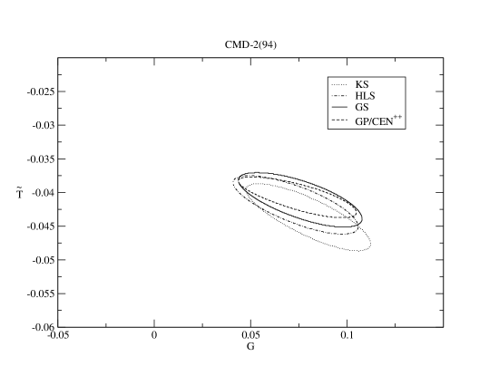
Figure 1: CMD-2(94) $G$ and $\tilde{T}$ one-sigma regions.

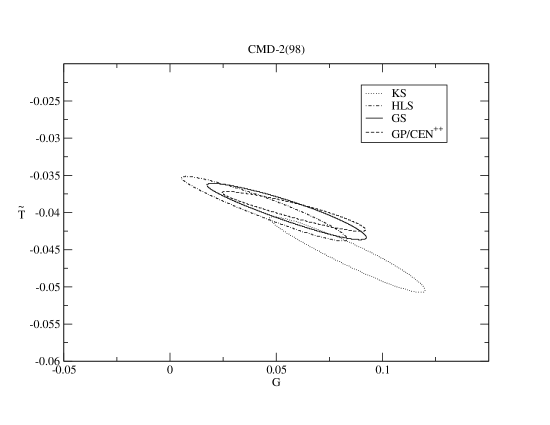
Figure 2: CMD-2(98) $G$ and $\tilde{T}$ one-sigma regions.

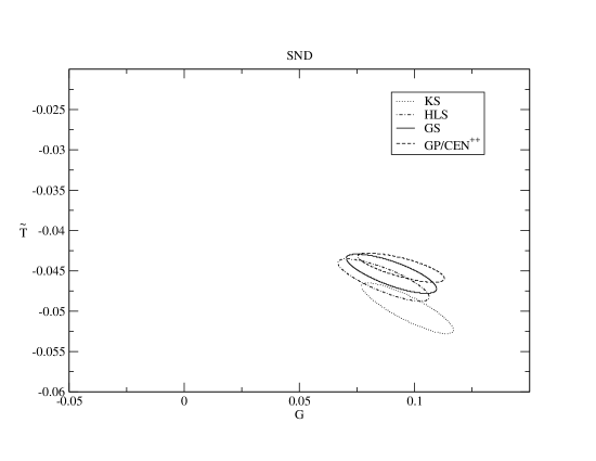
Figure 3: SND $G$ and $\tilde{T}$ one-sigma regions.

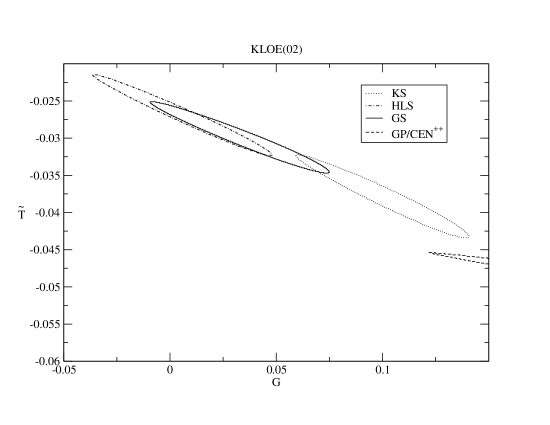
Figure 4: KLOE $G$ and $\tilde{T}$ one-sigma regions.

As Figures 1–4 show, it is possible to constrain $\tilde{T}$ rather well. With the prescription above for handling averages and uncertainties, we obtain

$$\tilde{T}=-0.044\pm 0.006_{model}\pm 0.002_{data}.$$

The consistency across different models for each data set is actually quite good.

The determination of $G$ is less precise, with the prescription above for determining the average across models and model-dependence uncertainty yielding

$$G=0.080\pm 0.026_{model}\pm 0.015_{data}.$$

For comparison, the uncorrected SND analysis snd05pipi , using a model very similar in form to the KS model described in Section II, reported $G=0.11\pm 0.01$, consistent with our result, $G=0.10\pm 0.02$, for the SND+KS case. The present analysis favors a non-vanishing $G$, as expected on general grounds, with a vanishing $G$ lying $\sim 2\sigma$ away from our central value. An improved determination of the Orsay phase, particularly in the case of the KLOE data, is required to make further progress on this issue. To illustrate this point, and also because of the lingering KLOE shape discrepancy kloefootnote , if one omits the KLOE data from the experimental averages one obtains results with a slightly reduced model-dependence uncertainty,

$$\tilde{T}=-0.045\pm 0.004_{model}\pm 0.002_{data}$$

and

$$G=0.084\pm 0.022_{model}\pm 0.016_{data}.$$

The values for $G$ and $\tilde{T}$ obtained in Tables 6–9 imply, using the earlier definitions, and our prescription for combining the results corresponding to different models, the result

$$\tilde{\Pi}_{\rho\omega}(m_{\rho}^{2})=-4950\pm 530_{model}\pm 250_{data}\ {\rm MeV}^{2}$$ (30)

for the real part of $\Pi_{\rho\omega}(m_{\rho}^{2})$. The imaginary part of $\Pi_{\rho\omega}(m_{\rho}^{2})$ is, similarly, found to be $-8600\pm 2510_{model}\pm 1690_{data}\ {\rm MeV}^{2}$. The result is an estimate of the off-diagonal part of the physical $\rho-\omega$ self-energy matrix at the $\rho$ mass

$$\Pi_{\rho\omega}(m_{\rho}^{2})=(-4950\pm 780)+(-8600\pm 4200)i\;{\rm MeV}^{2},$$ (31)

where we have combined the model-dependence and experimental errors linearly. Modestly reduced uncertainties are again obtained if the KLOE(02) data is excluded in forming the combined result. Explicitly:

$$\Pi_{\rho\omega}(m_{\rho}^{2})=(-4950\pm 670)+(-8890\pm 4000)i\;{\rm MeV}^{2}.$$ (32)

This quantity is not to be confused with the sometimes quoted ‘effective’ $\rho-\omega$ mixing matrix element, which contains direct $\omega\rightarrow\pi\pi$ contributions.

The separation described here is possible only because the two contributions enter the form factor with different (but known) phases, as shown by Eq. 27. Experimental determination of the combined phase (the Orsay phase) then allows the magnitude of each contribution to be determined separately. Any improvement in the separation of the $\rho-\omega$ mixing and direct $\omega\rightarrow\pi\pi$ IB contributions thus requires corresponding improvements in the determination of the Orsay phase.

VI Conclusions

Recent experiments provide a much-improved characterization of the prominent $\rho-\omega$ interference shoulder in the $e^{+}e^{-}\rightarrow\pi^{+}\pi^{-}$ cross-section, making precision analyses of isospin breaking in the $\rho-\omega$ system possible. Such an analysis is inherently dependent on the model chosen to represent the broad $\rho$ resonance contribution. By studying a range of models, all of which provide good fits to the data, we have shown that the model sensitivity of most fit parameters is generally greater than the statistical uncertainty associated with any given model. The only exception is the phase, ${\rm Arg}(\delta)$, of the parameter describing the strength of the $\omega$ contribution, for which the statistical uncertainty tends to be greater than the model sensitivity.

Any model sensitivity of course propagates to all quantities obtained from the fit parameters. The example discussed in Section IV is that of the $\rho-\omega$ interference contribution to the IB correction, $\left[\delta a_{\mu}\right]_{had}^{LO}$, required for incorporating hadronic $\tau$ decay data into the determination of the SM expectation for $[a_{\mu}]_{had}^{LO}$. Using our result, Eq. 18, the full IB correction obtained in Ref. dehz02 using the method of Ref. cen02 (see also footnote10 ), $\left[\delta a_{\mu}\right]^{LO}_{had}=(-13.8\pm 2.4)\times 10^{-10}$ (or $\left[\delta a_{\mu}\right]^{LO}_{had}=(-16.6\pm 1.6)\times 10^{-10}$ based on the recent analysis of Ref. davieretal09 ), receives only a small shift of $-0.4\times 10^{-10}$ ($+0.7\times 10^{-10}$) in its central value. The uncertainty in the size of the correction, however, increases by a much more significant $1.5\times 10^{-10}$. In arriving at the combined error, we have added the component associated with the model-dependence of the $\rho-\omega$ mixing contribution linearly to the other errors, for the reason discussed above. While the increased error does not serve to resolve the $\sim(17\pm 10)\times 10^{-10}$ passera07 ; jegerlehner09 ($\sim(11\pm 5)\times 10^{-10}$ davieretal09 ) $\tau$ vs. EM discrepancy which existed prior to the preliminary BaBar ISR results, it is nonetheless important to take into account in assessing the uncertainty in the IB corrections which must be applied if one wishes to use $\tau$ decay data in evaluating the SM contribution to $[a_{\mu}]^{LO}_{had}$.

The precision of the recent electroproduction data also allows new improved results for the (model-dependent) separation of contributions to $F_{\pi}(s)$ from $\rho-\omega$ mixing and direct (non-mixing) IB $\omega\to\pi\pi$ transitions. We estimate the ratio of the two-pion couplings of the isospin-pure $\omega$ and $\rho$ to be $G=0.080\pm 0.041$ where the uncertainty is conservatively chosen to encompass the experimental error intervals of all of the models considered. Further improvements in the determination of $G$ may be possible in future. As can be seen in Figures 1–4, the off-diagonal part of the vector meson self-energy matrix evaluated at the $\rho$ mass is very well constrained by the analysis. The central value we obtain for the real part is given in Eq. 30, where the uncertainty again conservatively encompasses the full ranges corresponding to all models and all data sets. Our central value of $\tilde{\Pi}_{\rho\omega}(m_{\rho}^{2})$ which is free of contamination from direct $\omega\rightarrow\pi\pi$ coupling contributions, and thus differs from the usually quoted ‘effective’ $\rho-\omega$ mixing matrix element obtained by ignoring such a direct coupling, should be used in place of the ‘effective’ matrix element results in meson-exchange models of IB NN scattering.

Further improvement of the separation of direct and mixing contributions requires a reduction in the uncertainty of the Orsay phase, which in turn requires a further increase in the precision of the $e^{+}e^{-}\to\pi^{+}\pi^{-}$ data in the $\rho-\omega$ interference region. This requires not only increased statistics but also very precise beam energy calibration such as that expected from VEPP-2000.

NOTE ADDED: Subsequent to the posting of this paper, the BaBar collaboration posted its results for the $e^{+}e^{-}\rightarrow\pi^{+}\pi^{-}$ cross-sections, obtained using the ISR method babarpipi09 . We will report the results of the analysis discussed here, applied to that data set, as soon as the data becomes publicly available.

- (1) R.R. Akhmetshin et al. (The CMD-2 Collaboration), Phys. Lett. B 527, 161 (2002); Phys. Lett. B 578, 285 (2004).
- (2) R. R. Akhmetshin et al. [CMD-2 Collaboration], Phys. Lett. B 648, 28 (2007).
- (3) A. Aloisio et al. (The KLOE Collaboration), Phys. Lett. B 606, 12 (2005).
- (4) F. Ambrosino et al. [KLOE Collaboration], Phys. Lett. B 670, 285 (2009).
- (5) M. N. Achasov et al., J. Exp. Theor. Phys. 101, 1053 (2005) [Zh. Eksp. Teor. Fiz. 101, 1201 (2005)].
- (6) M. N. Achasov et al., J. Exp. Theor. Phys. 103, 380 (2006) [Zh. Eksp. Teor. Fiz. 130, 437 (2006)].
- (7) L. M. Barkov et al., Nucl. Phys. B 256, 365 (1985).
- (8) V. E. Balakin et al., Phys. Lett. B 41, 205 (1972).
- (9) D. Benaksas et al., Phys. Lett. B 39, 289 (1972).
- (10) G. Barbiellini et al., Lett. Nuovo Cim. 6S2, 557 (1973) [Lett. Nuovo Cim. 6, 557 (1973)].
- (11) G.A. Miller, A.K. Opper and E.J. Stephenson, Ann. Rev. Nucl. Part. Sci. 56, 253 (2006).
- (12) K. Maltman, H.B. O’Connell, and A.G. Williams, Phys. Lett. B 376, 19 (1996).
- (13) G.W. Bennett et al. (The Muon Collaboration), Phys. Rev. Lett. 92, 161802 (2004).
- (14) M. Gourdin and E. de Rafael, Nucl. Phys. B 10, 667 (1969).
- (15) While estimates of based on the new data are consistent with one another, a discrepancy still exists between the KLOE kloe08 results for and those obtained by CMD-2 cmd203 ; cmd207 and SND snd05pipi ; snd06pipi in the region above the . The fact that this discrepancy is not yet understood kloe08 ; passera04 strikes a cautionary note.
- (16) M. Passera, J. Phys. G 31, R75 (2005).
- (17) M. Davier, Nucl. Phys. Proc. Suppl. 169, 288 (2007).
- (18) M. Passera, Nucl. Phys. Proc. Suppl. 169, 213 (2007).
- (19) K. Hagiwara, A. D. Martin, D. Nomura and T. Teubner, Phys. Lett. B 649, 173 (2007).
- (20) F. Jegerlehner and A. Nyffeler, Phys. Rep. 477, 1 (2009).
- (21) M. Davier et. al, arXiv:0906.5443 [hep-ph].
- (22) M. Davier (BaBar Coll.), Nucl. Phys. Proc. Suppl. 189, 222 (2009) For the powerpoint slides of this talk, follow the link at /tau08.inp.nsk.su/prog.php.
- (23) R. Alemany, M. Davier and A. Hocker, Eur. Phys. J. C 2, 123 (1998).
- (24) M. Davier and A. Hocker, Phys. Lett. B 419, 419 (1998); Phys. Lett. B 435, 427 (1998).
- (25) G. Colangelo, Nucl. Phys. Proc. Suppl. 131, 185 (2004).
- (26) J.F. de Troconiz and F.J. Yndurain, Phys. Rev. D 71, 073008 (2005).
- (27) A. Hocker, arXiv:hep-ph/0410081
- (28) R. Barate et al. (The ALEPH Collaboration), Z. Phys. C 76, 15 (1997).
- (29) K. Anderson et al. (The OPAL Collaboration), Eur. Phys. J. C 7, 571 (1999).
- (30) S. Anderson et al. (The CLEO Collaboration), Phys. Rev. D 61, 112002 (2000).
- (31) S. Schael et al. [ALEPH Collaboration], Phys. Rept. 421, 191 (2005).
- (32) M. Davier, A. Hocker and Z. Zhang, Rev. Mod. Phys. 78, 1043 (2006).
- (33) M. Fujikawa et al. [Belle Collaboration], Phys. Rev. D 78, 072006 (2008).
- (34) M. Davier, S. Eidelman, A. Hocker and Z. Zhang, Eur. Phys. J. C 27, 497 (2003).
- (35) M. Davier, S. Eidelman, A. Hocker and Z. Zhang, Eur. Phys. J. C 31, 503 (2003).
- (36) V. Cirigliano, G. Ecker and H. Neufeld, Phys. Lett. B 513, 361 (2001).
- (37) V. Cirigliano, G. Ecker and H. Neufeld, JHEP 0208, 002 (2002).
- (38) S. Ghozzi and F. Jegerlehner, Phys. Lett. B 583, 222 (2004).
- (39) F. Flores-Baez, A. Flores-Tlalpa, G. Lopez Castro and G. Toledo Sanchez, Phys. Rev. D 74, 071301 (2006).
- (40) A. Flores-Tlalpa, F. Flores-Baez, G. Lopez Castro and G. Toledo Sanchez, Nucl. Phys. Proc. Suppl. 169, 250 (2007).
- (41) K. Maltman and C. E. Wolfe, Phys. Rev. D 73, 013004 (2006).
- (42) K. Maltman, Phys. Lett. B 633, 512 (2006).
- (43) C.T.H. Davies et al. (The HPQCD Collaboration), Phys. Rev. D 78, 114507 (2008); K. Maltman, D. Leinweber, P. Moran and A. Sternbeck, Phys. Rev. D78, 114504 (2008).
- (44) K. Maltman and T. Yavin, Phys. Rev. D 78, 094020 (2008).
- (45) F. Guerrero and A. Pich, Phys. Lett. B 412, 382 (1997).
- (46) J.H. Kuhn and A. Santamaria, Z. Phys. C 48, 445 (1990).
- (47) M. Bando et al., Phys. Rev. Lett. 54, 1215 (1985).
- (48) G.J. Gounaris and J.J. Sakurai, Phys. Rev. Lett. 21, 244 (1968).
- (49) M. Benayoun et al., Eur. Phys. J. C 2, 269 (1998).
- (50) We thank Vincenzo Cirigliano for clarifying this point.
- (51) S. Eidelman, private communication.
- (52) See Ref. dehz02 for further details on the vacuum polarization corrections necessary to convert the cross-sections reported by various collaborations in the literature to the corresponding “bare” cross-section values.
- (53) Davier daviernote , working with the GS model, has noted that the and values obtained from fits to the bare and vacuum-polarization-dressed versions of the CMD-2 cross-sections differ by MeV. Similar shifts also occur for the other models. These shifts produce corresponding shifts in the interference contribution to . The versions associated with the fits to the bare cross-sections, quoted in the text, lie higher than those associated with the fit to the vacuum-polarization-dressed values by , depending on the model. The relevant versions for comparison to the data are, as explained by Davier, those obtained from the fit to the bare cross-sections daviernote . These are also the versions relevant to the determination of .
- (54) M. Davier, Nucl. Phys. Proc. Suppl. 131, 123 (2004).
- (55) Use of the recently posted Belle values for the mass and width of the belle08taupipi results in no significant difference in fit quality or in the values of the fit parameters.
- (56) The older PDG average value for the width of the is used with the GS model to ease comparison with the CMD-2 analyses. The fits are largely insensitive to the precise value of the width.
- (57) When quoting the earlier central value and uncertainty for , we use the result obtained in Ref. dehz02 , based on the same formalism as elaborated in Ref. cen02 , but with improved experimental inputs.
- (58) S.A. Coon and R.C. Barrett, Phys. Rev. C 36, 2189 (1987).
- (59) A. Bernicha, G. Lopez Castro and J. Pestieau, Phys. Rev. D 50, 4454 (1994).
- (60) W.-M. Yao et al. (Particle Data Group), J. Phys. G 33, 1 (2006) and 2007 partial update for the 2008 edition.
- (61) B. Aubert it et. al. (The BaBar Collaboration), arXiv:0908.3589 [hep-ex]