Infinite random geometric graphs

Abstract.

We introduce a new class of countably infinite random geometric graphs, whose vertices $V$ are points in a metric space, and vertices are adjacent independently with probability $p\in(0,1)$ if the metric distance between the vertices is below a given threshold. If $V$ is a countable dense set in $\mathbb{R}^{n}$ equipped with the metric derived from the $L_{\infty}$-norm, then it is shown that with probability $1$ such infinite random geometric graphs have a unique isomorphism type. The isomorphism type, which we call $GR_{n},$ is characterized by a geometric analogue of the existentially closed adjacency property, and we give a deterministic construction of $GR_{n}.$ In contrast, we show that infinite random geometric graphs in $\mathbb{R}^{2}$ with the Euclidean metric are not necessarily isomorphic.

1. Introduction

The last decade has seen the emergence of the study of large-scale complex networks such as the web graph consisting of web pages and the links between them, the friendship network on Facebook, and networks of interacting proteins in a cell. Several new random graph models were proposed for such networks, and existing models were modified in order to fit the data gathered from these real-life networks. See the books [3, 8] for surveys of such models. A recent trend in stochastic graph modelling is the study of geometric graph models. In geometric graph models, vertices are embedded in a metric space, and the formation of edges is influenced by the relative position of the vertices in this space. Geometric graph models have found applications in modelling wireless networks (see [12, 13]), and in modelling the web graph and other complex networks ([1, 11]). In real-world networks, the underlying metric space is a representation of the “hidden reality” that leads to the formation of edges. Thus, for the World Wide Web, web pages are embedded in a high dimensional topic space, where pages that are positioned close together in the space contain similar content.

The graph model we study is a variation on the random geometric graph, where vertices are chosen at random according to a given probability distribution from a given metric space, and two vertices are adjacent if the distance between the two vertices is no larger than some fixed real number. Random geometric graphs have been studied extensively in their own right (see, for example, [2, 9] and the book [15]).

Analysis of stochastic graph models usually focusses on asymptotic results, which hold for cases where the number of vertices is sufficiently large. An alternative approach is to study the infinite limit; that is, the infinite graph that results when the number of vertices reaches infinity. Studying the infinite limit is a well-known tool for studying scientific models, and it can help to recognize large-scale structure and long-term behaviour (see [4, 14]). In this paper, we study the infinite limit of a geometric graph model that is a geometric extension of the classic random graph model $G(\mathbb{N},p)$.

One of the most studied examples of an infinite limit graph arising from a stochastic model is the infinite random graph. The probability space $G(\mathbb{N},p)$ consists of graphs with vertices $\mathbb{N},$ so that each distinct pair of integers is adjacent independently with a fixed probability $p\in(0,1).$ Erdős and Rényi [10] discovered that with probability $1,$ all $G\in G(\mathbb{N},p)$ are isomorphic. A graph $G$ is existentially closed (or e.c.) if for all finite disjoint sets of vertices $A$ and $B$ (one of which may be empty), there is a vertex $z\notin A\cup B$ adjacent to all vertices of $A$ and to no vertex of $B.$ We say that $z$ is correctly joined to $A$ and $B.$ The unique isomorphism type of countably infinite e.c. graph is named the infinite random graph, or the Rado graph, and is written $R.$ See the surveys [6, 7] for additional background on $R.$

We now introduce the geometric graph model on which this paper is based. Consider a metric space $S$ with distance function

$$d:S\times S\rightarrow\mathbb{R},$$

$\delta\in{\mathbb{R}}^{+}$, a countable subset $V$ of $S$, and $p\in(0,1)$. The Local Area Random Graph $\mathrm{LARG}(V,\delta,p)$ has vertices $V,$ and for each pair of vertices $u$ and $v$ with $d(u,v)<\delta$, an edge is added independently with probability $p$. Note that $V$ may be either finite or infinite. The LARG model generalizes well-known classes of random graphs. For example, special cases of the $\mathrm{LARG}$ model include the random geometric graphs (where $p=1$), and the binomial random graph $G(n,p)$ (where $S$ has finite diameter $d$, and $\delta\geq d$).

In the case $V$ is infinite, our goals are to investigate what adjacency properties are satisfied by graphs generated by the LARG model, and determine when the model generates a unique isomorphism type of countable graph. We prove that with probability $1$, graphs in $\mathrm{LARG}(V,\delta,p)$ satisfy a certain adjacency property which is a metric analogue of the e.c. property; see Theorem 1. The so-called geometric e.c. property requires that vertices $z$ correctly joined to $A$ and $B$ may be found as close as we like to points in $V.$ Explicit examples of graphs with the geometric e.c. property are given in Theorem 2. For metric spaces such as $\mathbb{R}^{n}$ with the $L_{\infty}$-metric, the geometric e.c. property gives rise to a unique isomorphism type of graph; see Theorems 6, 9, and 10. The main tool here is a generalization of isometry called a step-isometry. Our results are sensitive to the metric used. Non-isomorphism results for other metrics are given in Section 4. In particular, we show in Theorem 15 that in $\mathbb{R}^{2}$ with the Euclidean metric, there exist non-isomorphic geometric e.c. graphs.

All graphs considered are simple, undirected, and countable unless otherwise stated. If $S$ is a set of vertices in $G$, then we use the notation $G[S]$ for the subgraph of $G$ induced by $S.$ We use the notation $G\leq H$ if $G$ is an induced subgraph of $H.$ We refer to an isomorphism type as isotype, and denote isomorphic graphs by $G\cong H.$ Given a metric space $S$ with distance function $d$, define the (open) ball of radius $\delta$ around $x$ by

$$B_{\delta}(x)=\{u\in S:d(u,x)<\delta\}.$$

We will sometimes just refer to $B_{\delta}(x)$ as a ball. A subset $V$ is dense in $S$ if for every point $x\in S$, every ball around $x$ contains at least one point from $V$. We refer to $u\in S$ as points or vertices, depending on the context. Throughout, let $\mathbb{N}$ denote the non-negative natural numbers, and $\mathbb{N}^{+}$ denote the positive natural numbers. For a reference on graph theory the reader is directed to [16], while [5] is a reference on metric spaces.

2. Geometrically e.c. graphs

As noted in the introduction, the unique isotype of the infinite random graph $R$ is characterized by the e.c. property. In this section we define a geometric analogue of this property. As will be demonstrated in Section 3, this property characterizes the unique isotype of graphs obtained from countable dense sets in ${\mathbb{R}}^{n}$, provided we consider a particular metric.

Let $G=(V,E)$ be a graph whose vertices are points in the metric space $S$ with metric $d.$ The graph $G$ is geometrically e.c. at level $\delta$ (or $\delta$-g.e.c.) if for all $\delta^{\prime}$ so that $0<\delta^{\prime}<\delta$, for all $x\in V$, and for all disjoint finite sets $A$ and $B$ so that $A\cup B\in B_{\delta}(x)$, there exists a vertex $z\not\in A\cup B\cup\{x\}$ so that

• $z$ is correctly joined to $A$ and $B$,

• for all $u\in A\cup B$, $d(u,z)<\delta$, and

• $d(x,z)<\delta^{\prime}$.

This definition implies that $V$ is dense in itself. Also, if $G$ is $\delta$-e.c., then $G$ is $\delta^{\prime}$-e.c. for any $\delta^{\prime}<\delta$.

The geometrically e.c. property bears clear similarities with the e.c. property. The important differences are that a correctly joined vertex must exist only for sets $A$ and $B$ which are contained in an open ball with radius $\delta$ and centre $x$, and it must be possible to choose the vertex $z$ correctly joined to $A$ and $B$ arbitrarily close to $x$. See Figure 1.

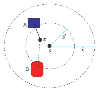
Figure 1. The $\delta$-g.e.c. property.

Theorem 1.

Let $(S,d)$ be a metric space and $V$ a countable subset of $S$ which is dense in itself. If $\delta>0$ and $p\in(0,1),$ then with probability $1,$ $\mathrm{LARG}(V,\delta,p)$ is $\delta$-e.c.

Proof.

Fix $x\in V$, disjoint finite subsets $A$ and $B$ in $B_{\delta}(x)\cap(V\setminus\{x\})$, and $0<\delta^{\prime}<\delta$. Let

$$\beta=\max\{d(x,v):v\in A\cap B\}.$$

Then $\beta<\delta$. Let $\epsilon=\min\{\delta-\beta,\delta^{\prime}\}$. Consider the set $Z=B_{\epsilon}(x)\cap V.$ Note that $\epsilon$ is chosen so that for any $z\in Z$, $d(z,x)<\delta^{\prime}$, and for all $u\in A\cup B$,

$$d(u,z)<d(u,x)+d(x,z)<\beta+\epsilon\leq\delta.$$

For any graph $G$ in $\mathrm{LARG}(V,\delta,p)$, the probability that any vertex $z\in Z$ is correctly joined to $A$ and $B$ equals $p^{|A|}(1-p)^{|B|}$. The probability that no vertex in $Z$ is correctly joined to $A$ and $B$ equals

$$P=\prod_{z\in Z}1-\left(p^{|A|}(1-p)^{|B|}\right).$$

Since $V$ is dense in itself, $Z$ contains infinitely many points; hence, $P=0.$ As there are only countably many choices for $x$, $A$, and $B$, and a countable union of measure $0$ sets is measure $0$, the proof follows. ∎

A graph $G=(V,E)$ whose vertices are points in the metric space $(S,d)$ has threshold $\delta$ if for all edges $uv\in E$, $d(u,v)<\delta$. A graph that is geometrically g.e.c. at level $\delta$ and has threshold $\delta$ is called a geometric $\delta$-graph. By definition, a graph $G$ generated by $\mathrm{LARG}(V,\delta,p)$ has threshold $\delta$, and, if $V$ is countable and dense in itself, $G$ is a geometric $\delta$-graph. Thus, this random graph model generates geometric $\delta$-graphs.

We construct geometric $\delta$-graphs deterministically as follows. Given $\delta>0$, a countable set $V$ which is dense in itself, and a linear ordering $\sigma:{\mathbb{N}}\rightarrow V$ of $V$, define $GR(V,\delta,\sigma)$ as the limit of a chain of finite graphs $R_{t}$, where $R_{t}\leq R_{t+1}$ for any $t>1$, and $\{\sigma(i):1\leq i\leq t\}\subseteq V(R_{t})$. Let $R_{1}$ be the trivial graph with vertex set $\sigma(1)$. Assume that $R_{t}$ is defined and $\{\sigma(i):1\leq i\leq t\}\subseteq V(R_{t}).$

We now define $R_{t+1}.$ Enumerate all pairs $(A,x)$ so that $A\subseteq V(R_{t})$ and $x\in V(R_{t})\setminus A$ so that $A\subseteq B_{\delta}(x)$, via a lexicographic ordering based on $\sigma$. For each pair $(A,x)$, in order, choose $z=z_{A,x}$ to be the least index point in $V$ (according to $\sigma$) such that $z$ has not been chosen for any previous pairs $(A,x)$,

$$B_{\delta}(z)\cap V(R_{t})=B_{\delta}(x)\cap V(R_{t}),$$ (2.1)

and

$$d(z,x)<\min\{1/t,\delta\}.$$

Note that such a vertex exists as $V$ is dense and $R_{t}$ is finite. Join $z$ to all vertices in $A$ and to no other vertices of $R_{t}$. If necessary, add $\sigma(t+1)$ as an isolated vertex to form the graph $R_{t+1}.$ Observe that by (2.1), $GR(V,\delta,\sigma)$ is a $\delta$-threshold graph.

Theorem 2.

The graph $GR(V,\delta,\sigma)$ is $\delta$-g.e.c.

Proof.

To show that $GR(V,\delta,\sigma)=(V,E)$ is $\delta$-g.e.c., choose $0<\delta^{\prime}<\delta$, a vertex $x\in V,$ and disjoint sets $A,B\subseteq V\setminus\{x\}$ so that $A\cup B\subseteq B_{\delta}(x)$. Let $t>0$ be chosen so that $A\cup B\cup\{x\}\subseteq V(R_{t})$ and $1/t<\delta^{\prime}$. Let $z=z_{A,x}$ be the vertex in $R_{t+1}$ added to $R_{t}$ to extend $(A,x)$. Then $z$ is correctly joined to $A$ and $B$ and $d(x,z)<\delta^{\prime}$. ∎

It should be emphasized that we do not claim that the graphs $GR(V,\delta,\sigma)$ are the unique isotypes of $\delta$-g.e.c. graphs with vertex set $V.$ The theme of when two $\delta$-g.e.c. graphs are isomorphic will be explored in the next two sections.

Balls with radius $\delta$ in $\delta$-g.e.c. graphs contain copies of $R$, and hence, contain isomorphic copies of all countable graphs.

Theorem 3.

Let $U\subseteq S$ be so that $U\subseteq B_{\delta}(x)$ for some $x\in U.$ Then a $\delta$-g.e.c. graph with vertex set $U$ is e.c., and so is isomorphic to $R$.

Proof.

Let $G$ be a graph with vertex set $U$, where $U$ is as stated. Assume that $G$ is $\delta$-g.e.c. Let $A$ and $B$ be any pair of disjoint, finite subsets of $U\subseteq B_{\delta}(x)$, and let $0<\delta^{\prime}<\delta$. Then by the $\delta$-g.e.c. condition there exists a vertex $z\in B_{\delta^{\prime}}(x)\cap U$ so that $z$ is correctly joined to $A$ and $B$. ∎

The converse of Theorem 3 is false, in general. For example, consider the metric space $(\mathbb{R},d)$, where $d$ is the Euclidean metric, and let $\delta=1$. Fix $U$ an infinite clique in $R$, and let $U^{\prime}=V(R)\setminus U$. Embed the vertices of $U$ in ${\mathbb{R}}$ so that they form a set that is dense in $B_{1/2}(0)$. Embed the vertices of $U^{\prime}$ so that they form a set that is dense in $B_{1}(0)\setminus B_{1/2}(0)$. Now choose $y\in U$ so that $d(0,y)<1/4$, and let $A=\emptyset$, and $B=\{b\}$, where $b\in U\setminus\{y\}$. Let $\delta^{\prime}=1/4$. Note that $A\cap B\subseteq B_{1}(y)$. The embedding of the vertices of $R$ is such that all vertices in $B_{\delta^{\prime}}(y)$ are in $U$, so they are all adjacent to $b$. Thus, $B_{\delta^{\prime}}(y)$ does not contain any vertex correctly joined to $A$ and $B$, and thus, this embedding of $R$ is not $\delta$-g.e.c.

We finish with the following theorem which shows that there exists a close relationship between graph distance and metric distance in any graph that is $\delta$-g.e.c. We denote the closure of set $V$ in $S$ by $\overline{V}$. The set $W$ is convex if for every pair of points $x$ and $y$ in $W,$ there exists a point $z$ such that

$$d(x,z)+d(z,y)=d(x,z).$$

Theorem 4.

Let $G=(V,E)$ be geometric $\delta$-graph, and let $\overline{V}$ be convex. Let $u,v\in V$ so that $d(u,v)>\delta$. Then the graph distance between $u$ and $v$ in $G$ equals $\lfloor d(u,v)/\delta\rfloor+1$.

Theorem 4 directly leads to the following corollary, which supplies motivation for proofs of the isomorphism results in the next section, and will be used to prove the non-isomorphism results of the final section.

Corollary 5.

If $\overline{V}$ and $\overline{W}$ are convex, and there is a $\delta$-g.e.c. graph with vertices $V$ and a $\gamma$-g.e.c. graph with vertex set $W$ which are isomorphic via $f$, then for every pair of vertices $u,v\in V$,

$$\lfloor d(u,v)/\delta\rfloor=\lfloor d(f(u),f(v))/\gamma\rfloor.$$

We supply a generalization of isometry, motivated by Theorem 4 and Corollary 5. Given metric spaces $(S,d_{S})$ and $(T,d_{T})$, sets $V\subseteq S$ and $W\subseteq T$, and positive real numbers $\delta$ and $\gamma$, a step-isometry at level $(\delta,\gamma)$ from $V$ to $W$ is a surjective map $f:V\rightarrow W$ with the property that for every pair of vertices $u,v\in V,$

$$\lfloor d_{S}(u,v)/\delta\rfloor=\lfloor d_{W}(f(u),f(v))/\gamma\rfloor.$$

Every isometry is a step-isometry, but the converse is false, in general. For example, consider ${\mathbb{R}}$ with the Euclidean metric, let $\delta=\gamma=1$, and let $V=[0,1)$ and $W=[0,0.5)$. Then $f:V\rightarrow W$ given by $f(x)=x/2$ is a step-isometry, but is not an isometry.

Proof of Theorem 4.

Let $u,v\in V$. Let $k=\lfloor d(u,v)/\delta\rfloor+1$. By assumption, $k\geq 2$. Note that the choice of $k$ supplies that

$$(k-1)\delta\leq d(u,v)<k\delta.$$

Let $\ell$ be the graph distance of $u$ and $v,$ and note that $\ell>1$ since $G$ is a $\delta$-threshold graph.

To show that $\ell\geq k$, let $v_{0}v_{1}\cdots v_{\ell}$, where $v_{0}=u$, $v_{\ell}=v$, be a shortest path in $G$ from $u$ to $v$. Since $G$ has threshold $\delta$, $d(v_{i-1},v_{i})<\delta$ for $i=1,\dots,\ell$. Therefore,

$$(k-1)\delta \leq d(u,v)$$

$$\leq \sum_{i=1}^{\ell}d(v_{i-1},v_{i})$$

$$< \ell\delta,$$

and so $\ell\geq k$.

Next, we show how to construct a path of length $k$ from $u$ to $v$ in $G$, which will prove that $\ell\leq k$. Let $\epsilon=(k\delta-d(u,v))/k$, so $d(u,v)=k(\delta-\epsilon)$.

The set $\overline{V}$ is convex, so for every pair of vertices $x,y$, there exists a point $z\in\overline{V}$ so that $d(x,z)+d(z,y)=d(x,y)$. Using this property, we can obtain a sequence of points in $\overline{V}$ between $u$ and $v$ whose successive distances add up to $d(u,v)$, and which are at most $\epsilon/4$ apart. We can then choose vertices $x_{1},\dots,x_{k-1}$ from this sequence so that $d(x_{i},x_{i+1})<\delta-3\epsilon/4$ for $i=0,\dots,k-1$, where $x_{0}=u$ and $x_{k}=v$. For $1\leq i<k$, we may then find $w_{i}\in V$ so that $d(w_{i},x_{i})<\epsilon/8$. Letting $w_{0}=u$ and $w_{k}=v$, we have that for $i=0,\dots,k-1$,

$$d(w_{i},w_{i+1}) \leq d(w_{i},x_{i})+d(x_{i},x_{i+1})+d(x_{i+1},w_{i+1})$$ (2.2)

$$< \delta-3\epsilon/4+2\epsilon/8$$

$$< \delta-\epsilon/2.$$

Let $v_{0}=w_{0}=u$. Now we successively apply the $\delta$-e.c. property to choose $v_{i}\in V$ so that

• $d(v_{i},w_{i})<\epsilon/2$, and

• $v_{i}$ is adjacent to $v_{i-1}$ in $G$.

It then follows that $v_{0}v_{1}\cdots v_{k}$ is the desired path of length $k.$ More precisely, fix $i$, $1\leq i<k-1$, and assume $v_{i-1}$ exists so that item $(i)$ holds. Note that ($i$) and (2.2) implies that

$$d(w_{i},v_{i-1})\leq d(w_{i-1},w_{i})+d(w_{i-1},v_{i-1})<\delta.$$

Therefore, $v_{i-1}\in B_{\delta}(w_{i})$, and so we can find a vertex $v_{i}$ in $B_{\epsilon/2}(w_{i})$ which is adjacent to $v_{i-1}$. To choose the vertex $v_{k-1}$, let $v_{k}=w_{k}=v$. By the same argument as before, $d(w_{k-1},v_{k-2})<\delta$. Since $w_{k}=v_{k}$, $d(w_{k-1},v_{k})<\delta$. So $\{v_{k-2},v_{k}\}\subseteq B_{\delta}(w_{k-1})$. Therefore, there exist a vertex $v_{k-1}$ which is adjacent to $v_{k-2}$ and $v_{k}=v$. ∎

3. Isomorphism results

In this section we consider metric spaces where the geometric e.c. property gives a unique isotype of graph. We work in the space ${\mathbb{R}}$ with the usual metric defined by $d(x,y)=|x-y|$. (We will not mention this explicitly unless there is room for confusion.) The first result of the section—which serves as the template for more general results—is the following.

Theorem 6.

Let $V$ and $W$ be two countable dense subsets of ${\mathbb{R}}$, and let $\delta,\gamma>0$. If $G$ is a geometric $\delta$-graph with vertex set $V$ and $H$ is a geometric $\gamma$-graph with vertex set $W,$ then $G\cong H.$

The proof of the theorem (and others analogous to it in this section) build up an isomorphism as a step-isometry. In the proofs we use the following alternative characterization of step-isometries. Fix $\delta>0$ and $v_{0}\in{\mathbb{R}}$. Each $v\in{\mathbb{R}}$ may be uniquely represented as

$$v=v_{0}+q(v)\delta+r(v),$$

where $q(v)=\lfloor(v-v_{0})/\delta\rfloor$ and $0\leq r(v)<\delta$. In this representation, we will refer to $\delta$ as the offset, and to $v_{0}$ as the anchor. We will omit to state the anchor and offset explicitly wherever it is clear from the context. The term $r(v)$ is called the representative of $v$ and $q(v)$ the quotient.

Lemma 7.

Let $V$ and $W$ be subsets of ${\mathbb{R}}$, and let $\delta$ and $\gamma$ be two non-negative real numbers. A surjective function $f:V\rightarrow W$ is a step-isometry at level $(\delta,\gamma)$ if and only if the following two conditions hold.

1. For every $u,v\in V$, $r(u)\leq r(v)$ if and only if $r(f(u))\leq r(f(v)).$

2. For every $u\in V$, $q(u)=q(f(u))$,

where the representation of elements of $V$ has offset $\delta$ and that of $W$ has offset $\gamma$, and the anchor of the representation of $W$ is the image of the anchor of the representation of $V$ under $f$.

Proof.

Assume first that items (1) and (2) hold, and fix $u,v\in V$. Let $u^{\prime}=f(u)$ and $v^{\prime}=f(v)$. Assume without loss of generality that $v>u$; by hypothesis, this implies that $v^{\prime}>u^{\prime}$. Then $d(u,v)=v-u=(v-v_{0})-(u-v_{0})$, and so

$$d(u,v)=(v-v_{0})-(u-u_{0})=(q(v)-q(u))\delta+(r(v)-r(u)).$$

Hence,

$$\lfloor d(u,v)/\delta\rfloor=q(v)-q(u)-s,$$

where $s=0$ if $r(v)\geq r(u)$, and $s=1$ otherwise. Similarly,

$$\lfloor d(u^{\prime},v^{\prime})/\gamma\rfloor=q(v^{\prime})-q(u^{\prime})-s^{\prime},$$

where $s^{\prime}=0$ if $r(v^{\prime})\geq r(u^{\prime})$, and $s^{\prime}=1$ otherwise. By hypothesis, we have that $s=s^{\prime}$ and $q(v)-q(u)=q(v^{\prime})-q(u^{\prime})$. It follows that $f$ is a step-isometry at level $(\delta,\gamma)$.

Now assume that $f$ is a step-isometry at level $(\delta,\gamma)$. Let $v_{0}\in V$ and $w_{0}\in W$ be so that $f(v_{0})=w_{0}$ and consider the representations of elements of $V$ and $W$ with offsets $\delta$ and $\gamma$, and anchors $v_{0}$ and $w_{0}$, respectively.

Condition (2) follows immediately from the definition of step-isometry. For the proof of (1), fix any $u,v\in V$, and let $u^{\prime}=f(u)$ and $v^{\prime}=f(v)$. Then

$$\lfloor d(u,v)/\delta\rfloor=\lfloor q(v)-q(u)+(r(v)-r(u))/\delta\rfloor=q(v)-q(u)-s,$$

where $s=-\lfloor(r(v)-r(u))/\delta\rfloor$ ; similarly, $\lfloor d(u^{\prime},v^{\prime})/\gamma\rfloor=q(v^{\prime})-q(u^{\prime})-s^{\prime}$, where $s^{\prime}=-\lfloor(r(v^{\prime})-r(u^{\prime}))/\delta\rfloor$. Since $f$ is a step-isometry, $s=s^{\prime}$. If $s=s^{\prime}=0$, then both $r(v)\geq r(u)$ and $r(v^{\prime})\geq r(u^{\prime})$; if $s=s^{\prime}=1$, then $r(v)<r(u)$ and $r(v^{\prime})<r(u^{\prime})$. Thus item (1) holds. ∎

Proof of Theorem 6.

The proof follows using a variant of the back-and-forth method (used to show that $R$ is the unique isotype of e.c. graph). Let $V=\{v_{i}:i\geq 0\}$ and $W=\{w_{i}:i\geq 0\}$. For $i\geq 0$, we inductively construct a sequence of pairs of sets $(V_{i},W_{i})$ and isomorphisms $f_{i}:G[V_{i}]\rightarrow H[W_{i}]$, so that for all $i\geq 1$, $v_{i}\in V_{i}$, $w_{i}\in W_{i}$, $V_{i}\subseteq V_{i+1}$ and $W_{i}\subseteq W_{i+1}$, and $f_{i+1}$ extends $f_{i}$. It follows that

$$\bigcup_{i\in\mathbb{N}}f_{i}:G\rightarrow H$$

is an isomorphism. As an additional induction hypothesis we require that $f_{i}$ is a step-isometry from $V_{i}$ to $W_{i}$ at level $(\delta,\gamma)$. Specifically, we maintain conditions in items (1) and (2) from Lemma 7, where the representation of elements of $V$ has offset $\delta$ and anchor $v_{0}$, and the representation of elements of $W$ has offset $\gamma$ and anchor $w_{0}$.

Let $V_{0}=\{v_{0}\}$, $W_{0}=\{w_{0}\},$ and define $f_{0}$ by $f_{0}(v_{0})=w_{0}.$ Then $q(v_{0})=q(w_{0})=0$ and $r(v_{0})=r(v_{0}^{\prime})=0$, so the base case of the induction follows. For the induction step, fix $i\geq 0$. To construct $f_{i+1}$ from $f_{i}$ we first go forth by finding an image of $v_{i+1}$. In the following, $f$ refers to $f_{i}$ and $v=v_{i+1}$.

Define

$$a = \max\{r(f(u)):u\in V_{i}\mbox{ and }r(u)\leq r(v)\},$$

$$b = \min\{r(f(u)):u\in V_{i}\mbox{ and }r(u)>r(v)\}.$$

We claim that $a<b$. Namely, let $u_{a}$ and $u_{b}$ be the elements in $V_{i}$ for which the maximum and minimum that define $a$ and $b$ are attained, respectively. Thus, $r(f(u_{a}))=a$ and $r(f(u_{b}))=b$. By definition, $r(u_{a})\leq r(v)<r(u_{b})$. By the induction hypothesis (specifically, item (1) from Lemma 7), this implies that $a=r(f(u_{a}))<r(f(u_{b}))=b$.

In order to maintain the induction hypothesis, $r(f(v))$ must lie in $[a,b)$, and $q(f(v))$ must equal to $q(v)$. Let $k=q(v)$, and consider the interval

$$I=(k\gamma+a,k\gamma+b).$$

Any vertex in $I$ will qualify as a candidate for $f(v),$ so that $f_{i+1}$ is a step-isometry at level $(\delta,\gamma).$ We must then find a vertex in $I$ that will also guarantee that $f$ is an isomorphism, by making sure it has the correct neighbours. For this, we apply the $\gamma$-g.e.c. condition of $H$.

In order to apply the $\gamma$-g.e.c. condition, we need to ensure that the images of all neighbours of $v$ in $V_{i}$ lie in a $\gamma$-ball. Since $G$ has threshold $\delta$, we consider all vertices of $V_{i}$ that lie in a $\delta$-ball around $v$. Let $Y=B_{\delta}(v)\cap V_{i}$, and fix $x\in I\cap W$. Such a vertex $x$ exists since $W$ is dense in ${\mathbb{R}}$. By definition of $I$, $q(x)=k$. We claim that

$$f(Y)\subseteq B_{\gamma}(x).$$ (3.1)

To prove this, let $u\in Y.$ Since $q(v)=k$ and $d(u,v)<\delta$, it follows that $|q(u)-k|\leq 1$. Hence, $q(u)$ is one of $k,$ $k-1,$ or $k+1.$

If $q(u)=k,$ then $q(f(u))=k$ by induction hypothesis, so $d(f(u),x)<\gamma$. If $q(u)=k-1$, then $r(u)>r(v)$, so $r(f(u))>b$ by definition of $b$. Hence,

$$d(f(u),x) = x-f(u)$$

$$< k\gamma+b-(k-1)\gamma-r(f(u))$$

$$< \gamma.$$

The final case is when $q(u)=k+1.$ Then $r(f(u))\leq a$, so we have that

$$d(f(u),x) = f(u)-x$$

$$< (k+1)\gamma+r(f(u))-k\gamma-a$$

$$\leq \gamma.$$

In all cases, $f(u)\in B_{\gamma}(x),$ and (3.1) follows.

Since $G$ has threshold $\delta$, $N(v)\cap V_{i}\subseteq Y$. Now let $A=f(N(v)\cap V_{i})$ and $B=(W_{i}\cap B_{\delta}(x))\setminus A$. Then $A\cap B\subseteq B_{\gamma}(x)\cap W_{i}$. Let $\epsilon>0$ be chosen such that $B_{\epsilon}(x)\subseteq I$. We now use the $\gamma$-e.c. property of $H$ to find a point $z\in B_{\epsilon}(x)$ which is adjacent to all vertices in $A$ and no other vertices of (the finite set) $W_{i}$. Thus, we can add $z$ to $W_{i}$ to form $W_{i+1}$ and add $v$ to $V_{i}$ to form $V_{i+1}$, and set $f_{i+1}(v)=z$. Observe that $f_{i+1}$ is an isomorphism.

To finish the induction step, if $w_{i+1}\not\in W_{i+1}$ then we may go back, by finding an image $z=f^{-1}_{i+1}(w_{i+1})$ in an analogous fashion. We then add $z$ to $V_{i+1}$, and maintain that $f_{i+1}$ is an isomorphism. ∎

The proof of the following corollary is now immediate.

Corollary 8.

For all countable dense subsets $V$ of ${\mathbb{R}}$, $\delta>0$, and $p\in(0,1),$ with probability $1$, there is a unique isotype of graph, written $GR_{1},$ in $\mathrm{LARG}(V,\delta,p)$.

The isomorphism type of $GR_{1}$ does not depend on the choices of $V$, $\delta$ or $p$; moreover, the same result holds for any 1-dimensional normed vector space with the metric derived from the norm. For this reason, we name $GR_{1}$ the infinite random geometric graph of dimension 1. Note that $GR_{1}$ has infinite diameter (unlike $R$, which has diameter $2$). Note that, for any countable set $V\subseteq{\mathbb{R}}$, any ordering $\sigma$ of $v$, and any real $\delta>0$, the deterministic construction process $R(V,\sigma,\delta)$ described in the previous section gives explicit representations of $GR_{1}$.

We may extend Theorem 6 to sets that are not necessarily dense in all ${\mathbb{R}}$. The only additional condition required is that there exists a step-isometry between the two sets. For example, consider the rational intervals $V=[a,b)$ and $W=[a^{\prime},b^{\prime})$, where $\lfloor(b-a)/\delta\rfloor=\lfloor(b^{\prime}-a^{\prime})\gamma\rfloor$. Consider the bijective map $f:V\rightarrow W$ defined by

$$f(x)=\left\{\begin{array}[]{ll}a^{\prime}+q(x)\gamma+r(b^{\prime})r(x)/r(b)&\mbox{ if }r(x)\leq r(b)\\ a^{\prime}+(q(x)+1)\gamma+(\gamma-r(b^{\prime}))(\delta-r(x))/(\delta-r(b))&\mbox{ if }r(x)>r(b),\end{array}\right.$$

where $q(x)$, $r(x)$ and $r(b)$ refer to the representation of elements $V$ with offset $\delta$ and anchor $a$, and $r(b^{\prime})$ refers to the representation of elements $W$ with offset $\gamma$ and anchor $a^{\prime}$. In other words, $f$ is a convex mapping of the intervals $[a+k\delta,a+k\delta+r(b))$, $k=0,1,\dots,q(b)$, to the intervals $[a^{\prime}+k\gamma,a^{\prime}+k\gamma+r(b^{\prime}))$, respectively, and of the intervals $[a+r(b)+k\delta,a+(k+1)\delta)$ to the intervals $[a^{\prime}+r(b^{\prime})+k\gamma,a^{\prime}+(k+1)\gamma)$. It is straightforward to verify that $f$ is a step-isometry at level $(\delta,\gamma)$, so any geometric $\delta$-graph and geometric $\gamma$ graph with vertex sets $V$ and $W$, respectively, are isomorphic. Another setting we consider is where $V$ and $W$ are disjoint unions of rational intervals for which there exists a step-isometry between the endpoints of the intervals of $V$ to the endpoints of the intervals of $W$.

Theorem 9.

Let $V$ and $W$ be two countable subsets of ${\mathbb{R}}$, and let $\delta,\gamma>0$. Let $F$ be a bijective step-isometry from $V$ to $W$ at level $(\delta,\gamma)$. If $G$ is a geometric $\delta$-graph with vertex set $V$ and $H$ is a geometric $\gamma$-graph with vertex set $W,$ then $G\cong H.$

Proof.

Let $V=\{v_{i}:i\geq 0\}$ and $W=\{w_{i}:i\geq 0\}$, where $w_{i}=F(v_{i})$. As in the proof of Theorem 6, we inductively construct a sequence of pairs of sets $(V_{i},W_{i})$ ($i\geq 0$) and isomorphisms $f_{i}:G[V_{i}]\rightarrow H[W_{i}]$, so that for all $i\geq 1$, $v_{i}\in V_{i}$, $w_{i}\in W_{i}$, $V_{i}\subseteq V_{i+1}$ and $W_{i}\subseteq W_{i+1}$, and $f_{i+1}$ extends $f_{i}$. As an additional part of the induction hypothesis, we require that $f_{i}$ satisfies the following three conditions.

1. For every $u,v\in V$, $r(u)\leq r(v)$ if and only if $r(f(u))\leq r(f(v)).$

2. For every $u,v\in V$, $r(u)\leq r(v)$ if and only if $r(f(u))\leq r(F(v)).$

3. For every $u\in V$, $q(u)=q(f(u))$.

The first two conditions are those stated in Lemma 7, so this implies that $f_{i}$ is a step-isometry at level $(\delta,\gamma).$ We can also conclude from this lemma that for all $u,v\in V$, $r(u)\leq r(v)$ if and only if $r(F(u))\leq r(F(v))$.

Let $V_{0}=\{v_{0}\}$ and $W_{0}=\{w_{0}\}$, and set $f_{0}(v_{0})=w_{0}$. Conditions (1) and (3) follow as in the proof of Theorem 6. Condition (2) follows from the fact that $w_{0}=F(v_{0}=f(v_{0})$. For the induction step, fix $i\geq 0$. we construct $f_{i+1}$ from $f_{i}$ by first finding an image of $v_{i+1}$. In the following, $f$ refers to $f_{i}$, and $v=v_{i+1}$.

Let

$$M_{a} = \{u:\,u\in V_{i}\mbox{ and }r(F(u))\leq r(F(v))\},$$

$$M_{b} = \{u:\,u\in V_{i}\mbox{ and }r(F(u))>r(F(v))\},$$

and

$$a = \max\{x:\,x=r(f(u))\mbox{ or }x=r(F(u))\mbox{ where }u\in M_{a}\},$$

$$b = \min\{x:\,x=r(f(u))\mbox{ or }x=r(F(u))\mbox{ where }u\in M_{b}\}.$$

We have that $a<b$, since the order of the representatives of vertices in $V_{i}$ is preserved under $f$ and under $F$. (See the similar argument in the proof of Theorem 6.)

In order to maintain conditions (1) and (2) of the induction hypothesis, $r(f(v))$ should lie in $[a,b)$, and because of condition (3), $q(f(v))$ must equal $q(v)$. Let $k=q(v)$, and consider the interval $I=(k\gamma+a,k\gamma+b)$. From the definition of $a$ and $b$ it follows that $F(v)\in I$.

The remainder of the proof is now analogous to the proof of Theorem 6 and so is only sketched here. Let $x=F(v)$. We can show that $f(B_{\delta}(v)\cap V_{i})\subseteq B_{\gamma}(x)$. We can then invoke the $\gamma$-g.e.c. condition of $H$ to find a vertex $z$ in $I$ which is correctly joined to the vertices in $W_{i}$ so that an isomorphism is maintained if we set $f(v)=w$. Finally, we finish the induction step by going back and finding a suitable image $f^{-1}(w_{i+1})$. ∎

Theorem 6 extends to $\mathbb{R}^{n}$ with $n>1,$ provided we use the product metric; that is, the metric derived from the $L_{\infty}$ norm, defined by:

$$d(u,v)=\max\{|v_{i}-u_{i}|\,:1\leq i\leq n\},$$

where $u_{i}$ denotes the $i$-th component of $u$. Hence, we obtain unique isotypes of infinite random geometric graphs in all finite dimensions. For the remainder of the section, $n$ is a positive integer, and $d$ is assumed to be the metric defined above.

Theorem 10.

Consider the metric space $({\mathbb{R}}^{n},d)$, where $d$ is the product metric defined above. Let $V$ and $W$ be two countable sets dense in ${\mathbb{R}}^{n}$, and let $\delta,\gamma>0$. If $G$ is a geometric $\delta$-graph with vertex set $V$ and $H$ is a geometric $\gamma$-graph with vertex set $W$, then $G\cong H$. In particular, for all choices of $V$ and $\delta$, there is unique isomorphism type of geometric $\delta$-graphs in $({\mathbb{R}}^{n},d)$, written $GR_{n}$.

Theorem 10 is sensitive to the choice of metric. In Section 4, we will show that the conclusion of Theorem 10 for $d$ the Euclidean metric fails even for $n=2.$ The following provides the key tool for our proof of Theorem 10. As the proof is straightforward generalization of Lemma 7, it is omitted.

Lemma 11.

Let $V$ and $W$ be subsets of ${\mathbb{R}}^{n}$ with the $L_{\infty}$-metric, let $v_{0}\in V$ and $w_{0}\in W$, and let $\delta$ and $\gamma$ be two non-negative real numbers.

Then a surjective function $f:V\rightarrow W$ is a step-isometry at level $(\delta,\gamma)$ if the following two conditions hold for all $u,v\in V$ and for all $i$, $1\leq i\leq n$:

1. $r(u_{i})\leq r(v_{i})$ if and only if $r(f(u)_{i})\leq r(f(v)_{i}).$

2. $q(u_{i})=q(f(u)_{i})$,

where the representation of the $i$-th coordinate of elements of $V$ has offset $\delta$ and anchor $(v_{0})_{i}$ the representation of the $i$-th coordinate of elements of $W$ has offset $\gamma$ and anchor $(w_{0})_{i}$,

Proof of Theorem 10.

Let $V=\{v_{i}:i\geq 0\}$ and $W=\{w_{i}:i\geq 0\}$. We inductively construct a sequence of pairs of sets $(V_{i},W_{i})$ ($i\geq 0$) and isomorphisms $f_{i}:G[V_{i}]\rightarrow H[W_{i}]$, so that for all $i\geq 1$, $v_{i}\in V_{i}$, $w_{i}\in W_{i}$, $V_{i}\subseteq V_{i+1}$ and $W_{i}\subseteq W_{i+1}$, and $f_{i+1}$ extends $f_{i}$. As an additional induction hypothesis we require that $f_{i}$ satisfies conditions (1) and (2) from Lemma 11.

As in the proof of Theorem 6, for the base case we take $V_{0}=\{v_{0}\}$, $W_{0}=\{w_{0}\}$ and $f_{0}(v_{0})=w_{0}$. For the induction step, fix $i\geq 0$. we construct $f_{i+1}$ from $f_{i}$ by first finding an image of $v_{i+1}$. In the following, $f$ refers to $f_{i}$, and $v=v_{i+1}$.

For all $j$, $1\leq j\leq n$, define

$$a_{j} = \max\{r(f(u)_{j}):u\in V_{i}\mbox{ and }r(u_{j})\leq r(v_{j})\},$$

$$b_{j} = \min\{r(f(u)_{j}):u\in V_{i}\mbox{ and }r(u_{j})>r(v_{j})\}.$$

In order to maintain the induction hypothesis, for all $j$, $r(f(v))_{j}$ should lie in interval $[a_{j},b_{j})$, and $q(f(v)_{j})$ should be equal to $q(v_{j})$. Let $k_{j}=q(v_{j})$, and consider the product set

$$I=\prod_{1\leq j\leq n}(k_{j}\gamma+a_{j},k_{j}\gamma+b_{j}).$$

Any vertex in $I$ will qualify as a candidate for $f(v)$ so that $f$ satisfies conditions (1) and (2) from Lemma 11. The remainder of the proof is analogous to that of Theorem 6, and so is omitted. ∎

A step-isometric isomorphism is an isomorphism of graphs that is a step-isometry. In the base step in the proof of Theorem 10, if we are given induced subgraphs $V_{0}$ and $W_{0}$ such that $f_{0}:V_{0}\rightarrow W_{0}$ is a step-isometric isomorphism, then the rest of the proof follows as before. Hence, we have the following corollary, which shows that the graphs $GR_{n}$ act transitively on step-isometric isomorphic induced subgraphs.

Corollary 12.

Let $G$ and $H$ be finite induced subgraphs of $GR_{n}$ for some positive integer $n$. A step-isometric isomorphism $f:G\rightarrow H$ extends to an automorphism of $GR_{n}.$

Deleting a point from a dense set $V$ in ${\mathbb{R}}^{n}$ gives another dense set. Hence, we have the following inexhaustibility property.

Corollary 13.

For all $n>0$ and vertices $x$ in $GR_{n}$, $GR_{n}-x\cong GR_{n}.$

We can combine Theorems 9 and 10 to obtain a result about isomorphisms between graphs with vertex sets in ${\mathbb{R}}^{n}$ if there exist a special type of map between the sets. Given a set $V\subseteq{\mathbb{R}}^{n}$, denote the $i$-th component set of $V$ as:

$$V_{i}=\{x_{i}:\,x\in V\}.$$

Theorem 14.

Consider the metric space $({\mathbb{R}}^{n},d)$, where $d$ is the product metric defined above. Let $V$ and $W$ be two countable sets in ${\mathbb{R}}^{n}$, and let $\delta,\gamma>0$. Assume that for all $1\leq i\leq n$, there exists a step-isometry at level $(\delta,\gamma)$ from $V_{i}$ to $W_{i}$. If $G$ is a geometric $\delta$-graph with vertex set $V$ and $H$ is a a geometric $\gamma$ graph with vertex set $W,$ then $G\cong H$.

The proof is a straightforward generalization of the proofs of Theorems 9 and 10, and is therefore omitted.

4. Non-isomorphism results for Euclidean space

The choice of metric plays an important role in our isomorphism results in Section 3. We demonstrate that there are non-isomorphic geometrically e.c. graphs in the plane with the usual Euclidean metric (denoted by $d$).

Theorem 15.

Let $V$ be a countable set dense in $({\mathbb{R}}^{2},d),$ and let $G$ and $H$ be two graphs generated by the model $\mathrm{LARG}(V,p)$, where $0<p<1$. Then with probability 1, $G\ncong H.$

We have the following corollary, which is the antithesis of the results in the previous section.

Corollary 16.

Let $V$ be a countable set dense in ${\mathbb{R}}^{2}$ equipped with the Euclidean metric, and $\delta>0$ fixed. Then there exist infinitely many pair-wise non-isomorphic $\delta$-g.e.c. graphs with vertex set $V.$

For the proof of Theorem 15, we rely on the following geometric lemma.

Lemma 17.

Let $V$ and $W$ be dense subsets of ${\mathbb{R}}^{2}$ equipped with the Euclidean metric. Then every step-isometry from $V$ to $W$ is an isometry.

Proof.

Assume for a contradiction that there is a step-isometry $f:V\rightarrow W$ at level $(\delta,\gamma)$ that is not an isometry. Without loss of generality, we assume that $\delta=\gamma=1$. For each $u\in V$, let $u^{\prime}=f(u)\in W$. Since $f$ is not an isometry, there must exist points $x_{1}$ and $x_{2}$ so that $d(x_{1},x_{2})\not=d(x_{1}^{\prime},x_{2}^{\prime})$. Since $f$ is a bijection, we may assume, without loss of generality, that $d(x_{1},x_{2})<d(x_{1}^{\prime},x_{2}^{\prime})$.

The proof follows by the following two claims. Given $x,y\in V$, define the discrepancy of $x,y$ as

$$D(x,y)=|d(x,y)-d(x^{\prime},y^{\prime})|.$$

The discrepancy is a measure of the error in the distance between pairs of points and their images under $f$. Since $f$ is a step-isometry, we have that $D(x,y)<1$ for all $x,y\in V.$

Claim 1.

For every $\epsilon>0$, if there exist points $x_{1},x_{2}\in V$ so that

$$D(x_{1},x_{2})=\epsilon>0$$

and $d(x_{1},x_{2})>40$, then there exist points $x_{3},x_{4}\in V$ so that

$$D(x_{3},x_{4})>2\epsilon.$$

Claim 2.

If there exist points $x_{1},x_{2}\in V$ so that

$$D(x_{1},x_{2})=\epsilon>0,$$

then there exist points $x_{3},x_{4}\in V$ so that

$$D(x_{3},x_{4})>3/4\epsilon$$

and $d(x_{3},x_{4})>40$.

To see how the lemma follows from the claims, note that by hypothesis, there are two points of $V$ with discrepancy $\epsilon>0$. By Claim 2, there are two points of $V$ with discrepancy at least $3/4\epsilon,$ and with distance at least $40$ apart. By Claim 1 there are points with discrepancy at least $3/2\epsilon$ apart. By induction, we obtain a sequence of pairs of points $\{y_{i},z_{i}\}$ of $V$ whose discrepancy equals $(3/2)^{i}\epsilon$ which tends to infinity in $i$. In particular, there are points $y,z$ of $V$ so that $D(y,z)>1$, which contradicts the fact that $f$ is a step-isometry.

We now prove Claim 1. We first define some constants that will be useful in the proof. Let

$$m=d(x_{1},x_{2})/2,\text{ and }k=\lfloor m\rfloor+1.$$

Choose

$$0<\xi<\epsilon^{2}/(2k).$$

Since $V$ is dense in ${\mathbb{R}}^{2}$, we can find points $x_{3}$ and $x_{4}$ in $V$ so that

$$k-\xi<d(x_{i},x_{j})<k\text{ for }i=1,2\text{ and }j=3,4.$$

So $x_{1},x_{3},x_{2},x_{4}$ are the vertices of a quadrilateral whose sides have length between $k-\xi$ and $k$. See Figure 2.

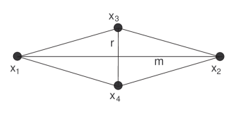
Figure 2. The quadrilateral formed by $x_{1},x_{3},x_{2},x_{4}$.

Let $r=d(x_{3},x_{4})/2$. The distance between $x_{3}$ and $x_{4}$ is smallest when all sides of the quadrilateral equal $k-\xi$, so using the Pythagorean theorem we have that

$$r^{2}\geq(k-\xi)^{2}-m^{2}\geq k^{2}-2k\xi-m^{2}\geq k^{2}-\epsilon^{2}-m^{2},$$ (4.1)

where the last step follows from the choice of $\xi$. (Note that the calculation above is only valid if we use the Euclidean metric.)

On the other hand, $x_{3}$ and $x_{4}$ are furthest when all sides of the quadrilateral equal $k$. Since $k\leq m+2$ and $m>20$, we obtain that

$$r^{2}\leq(m+2)^{2}-m^{2}=2m+1\leq m^{2}/4.$$ (4.2)

Now consider the quadrilateral formed by the images $x_{1}^{\prime},x_{2}^{\prime},x_{3}^{\prime}$, and $x_{4}^{\prime}$. Let

$$m^{\prime}=d(x_{1}^{\prime},x_{2}^{\prime})/2=m+\epsilon/2,\text{ and }r^{\prime}=d(x_{3}^{\prime},x_{4}^{\prime})/2.$$

See Figure 3.

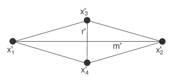
Figure 3. The quadrilateral formed by $x^{\prime}_{1},x^{\prime}_{3},x^{\prime}_{2},x^{\prime}_{4}$.

Since $f$ is a step-isometry,

$$d(x_{i}^{\prime},x_{j}^{\prime})<k\text{ for }i=1,2\text{ and }j=3,4.$$

Now $d(x_{3}^{\prime},x_{4}^{\prime})$ is largest when the quadrilateral has all sides equal to $k$. It follows that

$$(r^{\prime})^{2} \leq k^{2}-(m^{\prime})^{2}$$

$$= k^{2}-(m+\epsilon/2)^{2}$$

$$\leq k^{2}-m^{2}-m\epsilon$$

$$\leq r^{2}-m\epsilon+\epsilon^{2}$$

$$\leq (r-\epsilon)^{2}$$

where the third inequality follows from (4.1), and the last inequality follows from (4.2). In particular, $r^{\prime}\leq r-\epsilon.$ As

$$d(x_{3}^{\prime},x_{4}^{\prime})=2r^{\prime}\leq 2r-2\epsilon=d(x_{3},x_{4})+2\epsilon,$$

the proof of Claim 1 follows.

We now prove Claim 2. Let $m=d(x_{1},x_{2}),$ and assume $m<40$. Let $k=40$. Choose $c>0$ so that

$$10c/3+c^{2}\leq k\epsilon/4\text{ and }c<(2-\sqrt{3})\epsilon/8.$$ (4.3)

Further, choose points $x_{3},x_{4},x_{5},x_{6}\in V$ so that

$$k<d(x_{i},x_{j})<k+c,\text{ for }i,j\text{ equals }1,3\text{ or }1,5,\text{ or }2,4\text{ or }4,6,$$ (4.4)

$$k-c<d(x_{i},x_{j})<k,\text{ for }i,j\text{ equals }3,5\text{ or }4,6,$$ (4.5)

and

$$d(x_{3},x_{4})<d(x_{5},x_{6})<d(x_{3},x_{4})+c.$$ (4.6)

The choice of such points is possible since $V$ is dense. See Figure 4.

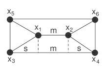
Figure 4. The figure formed by $x_{i},$ $1\leq i\leq 6$.

Subject to the given constraints, the points $x_{3}$ and $x_{4}$ are furthest apart when the distances achieve the upper bound of (4.4) and the lower bound from (4.5), and when $d(x_{3},x_{4})=d(x_{5},x_{6})$. Assume this to be the case. Then $x_{3},x_{4},x_{5},x_{6}$ form a rectangle, and the line segments $x_{1}x_{2}$, $x_{3}x_{4}$ and $x_{5}x_{6}$ are parallel.

For $i=1,2$, let $y_{i}$ be the orthogonal projection of $x_{i}$ on the line $x_{3}x_{4}$. Then $d(y_{1},y_{2})=d(x_{1},x_{2})=m$, and $d(x_{3},y_{1})=d(x_{4},y_{2})$; we will denote this distance by $s$. See Figure 4.

Hence, $d(x_{3},x_{4})=2s+m,$ and

$$s^{2}=(k+c)^{2}-1/4(k-c)^{2}=3/4(k^{2}+10kc/3+c^{2}),$$

and so

$$d(x_{3},x_{4})=\sqrt{3(k^{2}+(10/3)kc+c^{2})}+m.$$

The expression above is based on the case where $x_{3}$ and $x_{4}$ are furthest apart, and thus, it gives an upper bound for the general case. Combining this upper bound with the condition on $c$ given by (4.3), and with the assumption (4.6) we have for $i,j$ equals $3,4$ and $5,6$ that

$$d(x_{i},x_{j}) \leq m+c+\sqrt{3(k^{2}+(10/3)kc+c^{2})}$$

$$\leq m+c+\sqrt{3(k^{2}+k\epsilon/4)}$$

$$< m+c+\sqrt{3}(k+\epsilon/8)$$

$$< m+\sqrt{3}k+\epsilon/4,$$

where the first and last steps follow from (4.3).

We next consider the images of these points, and assume without loss of generality that $d(x_{3}^{\prime},x_{4}^{\prime})>d(x_{5}^{\prime},x_{6}^{\prime})$. Since $f$ is a step-isometry, $d(x_{i}^{\prime},x_{j}^{\prime})\geq k$ for $i,j$ equals $1,3$ or $1,5$ or $2,4$ or $2,6$, and $d(x_{i}^{\prime},x_{j}^{\prime})\leq k$ for $i,j$ equals $3,5$ or $4,6$. Moreover, by assumption $d(x_{1}^{\prime},x_{2}^{\prime})=m+\epsilon$. Now $x_{3}^{\prime}$ and $x_{4}^{\prime}$ are closest together when $d(x_{3}^{\prime},x_{4}^{\prime})=d(x_{5}^{\prime},x_{6}^{\prime})$ and $d(x_{i}^{\prime},x_{j}^{\prime})=k$ for all $i,j$ for which $|i-j|$ is even. As in the previous case, the line segments $x_{5}^{\prime}x_{6}^{\prime}$, $x_{1}^{\prime}x_{2}^{\prime}$, and $x_{3}^{\prime}x_{4}^{\prime}$ are parallel, and $x_{5}^{\prime}x_{6}^{\prime}x_{4}^{\prime}x_{3}^{\prime}$ is a rectangle. Under these assumptions we can compute $d(x_{3}^{\prime},x_{4}^{\prime})$ similarly to the computation for $d(x_{3},x_{4})$, and obtain that

$$d(x_{3}^{\prime},x_{4}^{\prime})=2(k\sqrt{3}/2)+(m+\epsilon).$$

Since our assumptions hold for the case where $x_{3}^{\prime}$ and $x_{4}^{\prime}$ are closest together, we have in general, for $i,j$ equal to $3,4$ and $5,6$, that

$$d(x_{i}^{\prime},x_{j}^{\prime})\geq k\sqrt{3}+m+\epsilon\geq d(x_{i},x_{j})+3\epsilon/4.\qed$$

A direct consequence of this lemma is the existence of many non-isomorphic g.e.c. graphs with vertex sets dense in ${\mathbb{R}}^{2}$, equipped with the Euclidean metric. A set $V$ in ${\mathbb{R}}^{2}$ is $\delta$-free if no pair of points in $V$ are distance $\delta$ apart. For instance, one may consider $\delta=1$, $V$ to be the set of all rational points in ${\mathbb{R}}^{2}$ which are $\delta$-free, and $W=V\cup\{(2^{1/4},0)\}$ (which is also $\delta$-free). It is straightforward to see there is no isometry from $V$ onto $W$. Hence, a $1$-g.e.c. graph on $V$ cannot be isomorphic to a $1$-g.e.c. graph on $W.$

In the following proof, we use the notation $\mathbb{P}(A)$ for the probability of an event $A.$

Proof of Theorem 15.

An enumeration $\{v_{i}:i\in{\mathbb{N}}^{+}\}$ of $V$ is good if $d(v_{i},v_{i+1})<\delta$ for all $i\in{\mathbb{N}}^{+}$ and $\{v_{1},v_{2},v_{3}\}$ are not collinear. We claim that a countable set $V$ dense in ${\mathbb{R}}$ has a good enumeration. For a positive integer $n$, we call $\{v_{i}:1\leq i\leq n\}$ a partial good enumeration of $V.$ We prove the claim by constructing a chain of partial good enumerations by induction. Using the density of $V,$ choose three points $\{v_{1},v_{2},v_{3}\}$ that are not collinear, so that each are within $\delta$ of each other. Let $V_{1}=\{v_{1},v_{2},v_{3}\}.$ Enumerate $V\setminus\{v_{1},v_{2},v_{3}\}$ as $\{u_{i}:i\geq 2\}.$ Starting from $V_{1}$, we inductively construct a chain of partial good enumerations $V_{n}$, $n\geq 1$, so that for $n\geq 2$, $V_{n}$ contains $\{u_{i}:2\leq i\leq n\}.$

We now want to form $V_{n+1}$ by adding $u=u_{n+1}$. If $u\in V_{n}$, then let $V_{n+1}=V_{n}$. Assume without loss of generality that $u\not\in V_{n}.$ Let $N=|V_{n}|$. If $d(v_{N},u)<\delta,$ then let $v_{N+1}=u$ and add it to $V_{n}$ to form $V_{n+1}.$ Otherwise, by the density of $V,$ choose a shortest finite path $P=p_{0},\dots,p_{\ell}$ of points of $V\setminus V_{n}$ starting at $v_{N}=p_{0}$ and ending at $u=p_{\ell}$ so that two consecutive points in the path are distance at most $\delta$. Then add the vertices of $P$ to $V_{n}$ to form $V_{n+1}$ and enumerate them so that $v_{N+i}=p_{i}$ for $i=0,1,\dots,\ell$. Taking the limit of this chain, $\bigcup_{n\geq 1}V_{n}$ is a good enumeration of $V$, which proves the claim.

Let $V=\{v_{i}:i\geq 1\}$ be a good enumeration of $V,$ and for any $n$, let $V_{n}=\{v_{i}:1\leq i\leq n\}.$ Let $G$ and $H$ be as stated. We say that two pairs $\{v,w\}$ and $\{v^{\prime},w^{\prime}\}$ of vertices are compatible if $\{v,w\}$ are adjacent in $G$ and $\{v^{\prime},w^{\prime}\}$ are adjacent in $H$ or $\{v,w\}$ are non-adjacent in $G$ and $\{v^{\prime},w^{\prime}\}$ are non-adjacent in $H$. For two pairs $\{v,w\}$ and $\{v^{\prime},w^{\prime}\}$ such that $d(v,w)=d(v^{\prime},w^{\prime})$, the probability that they are compatible equals

$$p^{*}=\left\{\begin{array}[]{ll}p^{2}+(1-p)^{2}&\text{if }d(v,w)<\delta\text{' and}\\ 1&\text{otherwise.}\end{array}\right.$$

By Corollary 5 and Lemma 17, any isomorphism between subgraphs of $G$ and $H$ must be an isometry. The images of three points in ${\mathbb{R}}^{2}$ that are not collinear determine the isometry. Let $A_{n}$ be the event that there exists a partial isomorphism $f$ from $G[V_{n}]$ into $H$ so that $f(\{v_{1},v_{2},v_{3}\})\subseteq V_{n}$, and let

$$A^{*}_{n}=\bigcap_{\nu\geq n}A_{\nu}.$$

Note that $A^{*}_{n}\subseteq A^{*}_{n+1}$ for all $n$.

Next, we estimate the probability of $A^{*}_{n}$. Note first that $\mathbb{P}(A^{*}_{n})\leq\mathbb{P}(A_{\nu})$ for all $\nu\geq n$. For any tuple $(u_{1},u_{2},u_{3})$ of three distinct vertices in $V_{n}$, let $C_{n}(u_{1},u_{2},u_{3})$ be the event that there exists a partial isomorphism $f$ from $G[V_{n}]$ to $H$ so that $f(v_{i})=u_{i}$ for $i=1,2,3$. Since the images of three points that are not collinear determine the isometry $f$, if $C_{n}$ happens then all pairs $(v_{i},v_{i+1})$ and $(f(v_{i}),f(v_{i+1}))$ must be compatible, for $1\leq i<n$. Thus,

$$\mathbb{P}(C_{n}(u_{1},u_{2},u_{3}))\leq(p^{*})^{n-1}.$$

Now

$$A_{n}=\bigcup_{u_{1},u_{2},u_{3}\in V_{n}}C_{n}(u_{1},u_{2},u_{3}),$$

so for $n\geq 3$ we have that $\mathbb{P}(A_{n})\leq n^{3}(p^{*})^{n-1}$, and

$$\mathbb{P}(A^{*}_{n})\leq\inf\{\nu^{3}(p^{*})^{\nu-1}:\nu\geq n\}=0.$$

If $B$ is the event that $G$ and $H$ are isomorphic, then

$$B\subseteq\bigcup_{n\in{\mathbb{N}}^{+}}A^{*}_{n}.$$

Since the union of countably many sets of measure zero has measure zero, we conclude that $\mathbb{P}(B)=0$, and thus, with probability $1,$ $G\ncong H.$ ∎

References

- [1] W. Aiello, A. Bonato, C. Cooper, J. Janssen, P. Prałat, A spatial web graph model with local influence regions, accepted to Internet Mathematics.
- [2] P. Balister, B. Bollobás, A. Sarkar, M. Walters, Highly connected random geometric graphs, Discrete Applied Mathematics 157 (2009) 309–320.
- [3] A. Bonato, A Course on the Web Graph, American Mathematical Society Graduate Studies Series in Mathematics, Providence, Rhode Island, 2008.
- [4] A. Bonato, J. Janssen, Infinite limits and adjacency properties of a generalized copying model, Internet Mathematics 4 (2009) 199-223.
- [5] V. Bryant, Metric Spaces: Iteration and Application, Cambridge University Press, Cambridge, 1985
- [6] P.J. Cameron, The random graph, In: Algorithms and Combinatorics 14 (R.L. Graham and J. Nešetřil, eds.), Springer Verlag, New York (1997) 333-351.
- [7] P.J. Cameron, The random graph revisited, In: European Congress of Mathematics Vol. I (C. Casacuberta, R. M. Miró-Roig, J. Verdera and S. Xambó-Descamps, eds.), Birkhauser, Basel (2001) 267-274.
- [8] F. Chung, L. Lu, Complex Graphs and Networks, American Mathematical Society, Providence, Rhode Island, 2006.
- [9] R. Ellis, X. Jia, C.H. Yan, On random points in the unit disk, Random Algorithm and Structures 29 (2006) 14–25
- [10] P. Erdős, A. Rényi, Asymmetric graphs, Acta Mathematica Academiae Scientiarum Hungaricae 14 (1963) 295-315.
- [11] A. Flaxman, A.M. Frieze, J. Vera, A geometric preferential attachment model of networks, Internet Mathematics 3 (2006) 187–205.
- [12] A.M. Frieze, J. Kleinberg, R. Ravi, W. Debany, Line of sight networks, Combinatorics, Probability and Computing 18 (2009) 145-163.
- [13] A. Goel, S. Rai, B. Krishnamachari, Monotone properties of random geometric graphs have sharp thresholds, Annals of Applied Probability 15 (2005) 2535-2552.
- [14] J. Kleinberg, R.D. Kleinberg, Isomorphism and embedding problems for infinite limits of scale-free graphs, In: Proceedings of the sixteenth annual ACM-SIAM symposium on Discrete algorithms, 2005.
- [15] M. Penrose, Random Geometric Graphs, Oxford University Press, Oxford, 2003.
- [16] D.B. West, Introduction to Graph Theory, 2nd edition, Prentice Hall, 2001.