Galactic Sun’s motion in the Cold Dark Matter, MOdified Newtonian Dynamics and MOdified Gravity scenarios

Abstract

We numerically integrate the equations of motion of the Sun in Galactocentric Cartesian rectangular coordinates for $-4.5$ Gyr $\leq t\leq 0$ in Newtonian mechanics with two different models for the Cold Dark Matter (CDM) halo, in MOdified Newtonian Dynamics (MOND) and in MOdified Gravity (MOG) without resorting to CDM. The initial conditions used come from the latest kinematical determination of the 3D Sun’s motion in the Milky Way (MW) by assuming for the rotation speed of the Local Standard of Rest (LSR) the recent value $\Theta_{0}=268$ km s^-1 and the IAU recommended value $\Theta_{0}=220$ km s^-1; the Sun is assumed located at 8.5 kpc from the Galactic Center (GC). For $\Theta_{0}=268$ km s^-1 the birth of the Sun, 4.5 Gyr ago, would have occurred at large Galactocentric distances ($12-27$ kpc depending on the model used), while for $\Theta_{0}=220$ km s^-1 it would have occurred at about $8.8-9.3$ kpc for almost all the models used. The integrated trajectories are far from being circular, especially for $\Theta_{0}=268$ km s^-1, and differ each other with the CDM models yielding the widest spatial extensions for the Sun’s orbital path.

1 Introduction

In several astrophysical systems like, e.g., spiral galaxies and clusters of galaxies a discrepancy between the observed kinematics of their exterior parts and the predicted one on the basis of the Newtonian dynamics and the matter detected from the emitted electromagnetic radiation (visible stars and gas clouds) was present since the pioneering studies by [Zwicky (1933)] (he postulated the existence of undetected, baryonic matter; today, it is believed that the hidden mass is constituted by non-baryonic, weakly interacting particles) on the Coma cluster, and by [Bosma (1981)] and [Rubin et al. (1982)] on spiral galaxies. More precisely, such an effect shows up in the galactic velocity rotation curves ([Persic & Salucci 1996a, 1996b]) whose typical pattern after a few kpc from the center differs from the Keplerian $1/\sqrt{r}$ fall-off expected from the usual dynamics applied to the electromagnetically-observed matter.

As a possible solution of this puzzle, the existence of non-baryonic, weakly-interacting Cold Dark (in the sense that its existence is indirectly inferred only from its gravitational action, not from emitted electromagnetic radiation) Matter (CDM) was proposed to reconcile the predictions with the observations ([Rubin 1983]) in the framework of the standard gravitational physics.

Oppositely, it was postulated that the Newtonian laws of gravitation have to be modified on certain acceleration scales to correctly account for the observed anomalous kinematics of such astrophysical systems without resorting to still undetected exotic forms of matter. One of the most phenomenologically successful modification of the inverse-square Newtonian law, mainly with respect to spiral galaxies, is the MOdified Newtonian Dynamics (MOND) ([Milgrom 1983a, 1983b, 1983c]) which, as we will see below, yields a $\approx 1/r$ gravitational force for very small accelerations.

Another alternative theoretical framework recently put forth to also explain, among other astrophysical and cosmological observations, the observed kinematics of the outskirts of galaxies without resorting to CDM is MOdified Gravity (MOG) ([Moffat & Toth 2008]) which yields a long-range Yukawa-like modification of the Newtonian inverse-square law.

In this paper we want to investigate the motion of the Sun in the Milky Way (MW) over timescales of the order of its lifetime, i.e. 4.5 Gyr, in CDM, MOND and MOG scenarios in view of the recent accurate measurements of the solar kinematical parameters ([Reid et al. 2009]). This may help in discriminating, at least in principle, the different theoretical scenarios examined; moreover, it will be interesting to see if the Galactic orbital motions of the Sun backward in time predicted by CDM, MOND and MOG are compatible with known and accepted knowledge concerning its formation and the evolution of the life in our planet. This may also yield an independent consistency test of the new kinematical determinations of MW ([Reid et al. 2009]). Finally, we note that the approach presented here may be used, in principle, also for other dynamical features.

2 The models used

2.1 The CDM NFW model

The CDM model tested by [Xue et al. (2008)] with several Blue Horizontal-Branch (BHB) halo stars consists of three components. Two of them are for the disk

$$U_{\rm disk}=-\frac{GM_{\rm disk}\left[1-\exp\left(-\frac{r}{b}\right)\right]}{r},$$ (1)

where $b$ is the disk scale length, and the bulge

$$U_{\rm bulge}=-\frac{GM_{\rm bulge}}{r+c_{0}},$$ (2)

where $c$ is the bulge scale radius. The third component is for the CDM NFW halo ([Navarro et al. 1996])

$$U_{\rm NFW}=-\frac{4\pi G\rho_{s}r_{\rm vir}^{3}}{c^{3}r}\ln\left(1+\frac{cr}{r_{\rm vir}}\right),$$ (3)

with $r_{\rm vir}$ is the radius parameter and

$$\rho_{s}=\frac{\rho_{\rm cr}\Omega_{\rm m}\delta_{\rm th}}{3}\frac{c^{3}}{\ln\left(1+c\right)-\frac{c}{1+c}},$$ (4)

in which $\Omega_{\rm m}$ is the fraction of matter (including baryons and DM) to the critical density, $\delta_{\rm th}$ is critical overdensity of the virialized system, $c$ is the concentration parameter, and

$$\rho_{\rm cr}=\frac{3H_{0}^{2}}{8\pi G}$$ (5)

is the critical density of the Universe determined by the Hubble parameter $H_{0}$ at redshift $0$. The values used for the parameters entering eq. (1) and eq. (2) are in Table 1;

Table 1: Parameters of the disk and bulge models by [Xue et al. (2008)].

$M_{\rm disk}$	$M_{\rm bulge}$	$b$	$c_{0}$
(M⊙)	(M⊙)	(kpc)	(kpc)
$5\times 10^{10}$	$1.5\times 10^{10}$	$4$	$0.6$

those entering eq. (3) are in Table 2.

Table 2: Parameters of the CDM NFW halo model by [Xue et al. (2008)]. The values quoted for $r_{\rm vir}$ and $c$ come from an average of those by [Xue et al. (2008)].

$\Omega_{\rm m}$	$\delta_{\rm th}$	$r_{\rm vir}$	$c$	$H_{0}$
-	-	(kpc)	(kpc)	(km s-1 Mpc-1)
$0.3$	$340$	$273.2$	$8.9$	65

2.2 The logarithmic CDM halo

Another model widely used consists of the [Miyamoto & Nagai (1975)] disk

$$U_{\rm disk}=-\frac{\xi GM_{\rm disk}}{\sqrt{x^{2}+y^{2}+\left(k+\sqrt{z^{2}+{B}^{2}}\right)^{2}}},$$ (6)

where $k$ and $B$ are the disk scale length and the disk scale height, respectively, the [Plummer (1911)] bulge

$$U_{\rm bulge}=-\frac{GM_{\rm bulge}}{r+C},$$ (7)

where $C$ is the bulge scale radius, and the logarithmic CDM halo ([Binney & Tremaine 1987])

$$U_{\rm halo}=v^{2}_{\rm halo}\ln\left(r^{2}+d^{2}\right),\ ({\rm spherical\ halo})$$ (8)

where $d$ is the DM halo scale length and $v_{\rm halo}$ describes the DM halo dispersion speed (which is related to the total DM halo mass). The parameters’s values are in Table 3.

Table 3: Parameters of the logarithmic CDM halo model; values by [Law et al. (2005)].

$\xi$	$k$	$B$	$C$	$v_{\rm halo}$	$d$
-	(kpc)	(kpc)	(kpc)	km s-1	(kpc)
$1$	$6.5$	$0.26$	$0.7$	$114$	$12$

The masses of the disk and the bulge used by [Law et al. (2005)] are those by [Johnston et al. (1999)]: $M_{\rm disk}=1\times 10^{11}$ M_⊙, $M_{\rm bulge}=3.4\times 10^{10}$ M_⊙ yielding a total baryonic mass of $M=1.34\times 10^{11}$ M_⊙; however, such a value is almost twice the most recent estimate ($M=6.5\times 10^{10}$ M_⊙) by [McGaugh (2008)] who includes the gas mass as well and yield $M_{\rm disk}=2.89\times 10^{10}$ M_⊙ and $M_{\rm bulge}=2.07\times 10^{10}$ M_⊙. The model of eq. (6)-eq. (8), with the parameters’ values by [Law et al. (2005)] and [Johnston et al. (1999)], has been recently used by [Willett et al. (2009)] to study the motion of the [Grillmair & Dionatos (2006)] tidal stellar stream at galactocentric distance of $r\approx 16-18$ kpc; [Read & Moore (2005)] used it to study the motion of the tidal debris of the Sagittarius dwarf at 17.4 kpc from the center of MW. More specifically, the CDM halo model of eq. (8) corresponds to a CDM halo mass

$$M_{\rm halo}=\frac{2v_{\rm halo}^{2}r^{3}}{G(r^{2}+d^{2})},$$ (9)

so that

$$M_{\rm halo}(r=60\ {\rm kpc})=3.5\times 10^{11}\ {\rm M}_{\odot},$$ (10)

in agreement with the value by [Xue et al. (2008)]

$$M_{\rm halo}(r=60\ {\rm kpc})=(4.0\pm 0.7)\times 10^{11}\ {\rm M}_{\odot}.$$ (11)

2.3 MOdified Newtonian Dynamics

MOND postulates that for systems experiencing total gravitational acceleration $A<A_{0}$, with ([Begeman et al. 1991])

$$A_{0}=(1.2\pm 0.27)\times 10^{-10}\ {\rm m\ s}^{-2},$$ (12)

$$A\rightarrow A_{\rm MOND}=-\frac{\sqrt{A_{0}GM}}{r}.$$ (13)

More precisely, it holds

$$A=\frac{A_{\rm Newton}}{\mu(X)},\ X\equiv\frac{A}{A_{0}};$$ (14)

$\mu(X)\rightarrow 1$ for $X\gg 1$, i.e. for large accelerations (with respect to $A_{0}$), while $\mu(X)\rightarrow X$ yielding eq. (13) for $X\ll 1$, i.e. for small accelerations. Concerning the interpolating function $\mu(X)$, it recently turned out that the simple form ([Famaey & Binney 2005])

$$\mu(X)=\frac{X}{1+X}.$$ (15)

yields very good results in fitting the terminal velocity curve of MW, the rotation curve of the standard external galaxy NGC 3198 ([Famaey & Binney 2005, Zhao & Famaey 2006, Famaey et al. 2007]) and of a sample of 17 high surface brightness, early-type disc galaxies ([Sanders & Noordermeer 2007]); eq. (14) becomes

$$A=\frac{A_{\rm Newton}}{2}\left(1+\sqrt{1+\frac{4A_{0}}{A_{\rm Newton}}}\right)$$ (16)

with eq. (15). Thus, in the following we will use eq. (16).

2.4 MOdified Gravity

MOG is a fully covariant theory of gravity which is based on the existence of a massive vector field coupled universally to matter. The theory yields a Yukawa-like modification of gravity with three constants which, in the most general case, are running; they are present in the theory’s action as scalar fields which represent the gravitational constant, the vector field coupling constant, and the vector field mass. An approximate solution of the MOG field equations by [Moffat & Toth (2009)] allows to compute their values as functions of the source’s mass. The resulting Yukawa-type modification of the inverse-square Newton’s law in the gravitational field of a central mass $M$ is

$$A=-\frac{G_{\rm N}M}{r^{2}}\left\{1+\alpha\left[1-\left(1+\mu r\right)\exp\left(-\mu r\right)\right]\right\},$$ (17)

with

$$\alpha \simeq \frac{M}{\left(\sqrt{M}+C^{{}^{\prime}}_{1}\right)^{2}}\left(\frac{G_{\infty}}{G_{\rm N}}-1\right),$$ (18)

$$\mu \simeq \frac{C_{2}^{{}^{\prime}}}{\sqrt{M}},$$ (19)

where $G_{\rm N}$ is the Newtonian gravitational constant and

$$G_{\infty} \simeq 20G_{\rm N},$$ (20)

$$C_{1}^{{}^{\prime}} \simeq 25,000\sqrt{{\rm M}_{\odot}},$$ (21)

$$C_{2}^{{}^{\prime}} \simeq 6,250\sqrt{{\rm M}_{\odot}}\ {\rm kpc}^{-1}.$$ (22)

Such values have been obtained by [Moffat & Toth (2009)] as a result of the fit of the velocity rotation curves of some galaxies in the framework of the searches for an explanation of the rotation curves of galaxies without resorting to CDM. The validity of eq. (17) in the Solar System has been recently questioned by [Iorio (2008)].

For $M=6.5\times 10^{10}$ M_⊙ we have the values of Table 4.

Table 4: MOG parameters $\alpha$ and $\lambda$ for $M=6.5\times 10^{10}$ M_⊙.

$\alpha$	$\lambda$
-	(kpc)
$16$	$41$

3 Solar motions backward in time

We will numerically integrate with MATHEMATICA the Sun’s equations of motion in Cartesian rectangular coordinates for $-4.5$ Gyr $\leq t\leq 0$ wit the initial conditions of Table 5; in it we use the recently estimated value $\Theta_{0}=268$ km s^-1 for the rotation speed of the Local Standard of Rest (LSR) ([Reid et al. 2009]).

Table 5: Galactocentric initial conditions for the Sun ([Reid et al. 2009]); the positive $y$ axis is directed from the Galactic Center (GC) to the Sun, the positive $x$ axis is directed toward the Galactic rotation, the positive $z$ axis is directed toward the North Galactic Pole (NGP). We have used ([Reid et al. 2009]) $\Theta_{0}=268$ km s^-1 for the rotation speed of LSR, and $U_{0}=10.3$ km s^-1, $V_{0}=15.3$ km s^-1, $W_{0}=7.7$ km s^-1 for the standard solar motions toward GC, $\ell=90$ deg and NGP, respectively; thus, with our conventions, $\dot{x}_{0}=V_{0}+\Theta_{0},\ \dot{y}_{0}=-U_{0},\ \dot{z}_{0}=W_{0}$. See Fig. 7 of ([Reid et al. 2009]).

$x_{0}$	$y_{0}$	$z_{0}$	$\dot{x}_{0}$	$\dot{y}_{0}$	$\dot{z}_{0}$
(kpc)	(kpc)	(kpc)	(km s-1)	(km s-1)	(km s-1)
$0$	$8.5$	$0.02$	$15.3+268$	$-10.3$	$7.7$

We will use both the NFW and logarithmic halo models for CDM which have been tested independently of the solar motion itself. In particular, we will numerically integrate the three scalar differential equations, written in cartesian coordinates, corresponding to the vector differential equation

$$\frac{{{d^{2}}}{\boldsymbol{r}}}{{{d}}{t^{2}}}=-\boldsymbol{\nabla}U,$$ (23)

where $U$ is the sum of eq. (1)-eq. (3) with the values of Table 2 in the first case (NFW), and of eq. (6)-eq. (8) with the values of Table 3 in the second case (logarithmic); we use the figures of Table 1 in both cases. For the two models of modified gravity considered we will put the cartesian components of eq. (16) (MOND) and eq. (17) (MOG) in the right-hand-sides of the differential equations to be integrated. Concerning MOND, let us note that Eq. (14), from which eq. (16) has been derived by means of eq. (15) for $\mu(X)$, strictly holds for co-planar, spherically and axially symmetric mass distributions; otherwise, the full modified (non-relativistic) Poisson equation ([Bekenstein & Milgrom 1984])

$$\boldsymbol{\nabla}\boldsymbol{\cdot}\left[\mu\left(\frac{|\boldsymbol{\nabla}U|}{A_{0}}\right)\boldsymbol{\nabla}U\right]=4\pi G\rho$$ (24)

must be used. However, in this case, the baryonic mass distributions of the bulge and the disk (see eq. (1)-eq. (2) and eq. (6)-eq. (7)) just satisfy the symmetry conditions that allow to use eq. (14). Moreover, $A_{\rm N}/A_{0}\approx 1$ for $M=6,5\times 10^{10}$ M_⊙. This allows to neglect the so-called External Field Effect (EFE) ([Sanders & McGaugh 2002, Milgrom 2008]) because it should amount to about $A_{\rm e}/A_{0}=0.01-0.02$ for MW ([Wu et al. 2008]). Indeed, it can be shown that, for eq. (15), the MOND acceleration, including EFE, is

$$A=\frac{A_{\rm N}}{2}\left[1-\frac{A_{\rm e}}{A_{\rm N}}+\sqrt{\left(1-\frac{A_{\rm e}}{A_{\rm N}}\right)^{2}+\frac{4A_{0}}{A_{\rm N}}\left(1+\frac{A_{\rm e}}{A_{0}}\right)}\right],$$ (25)

which just reduces to eq. (16) when $A_{\rm e}\ll A_{\rm N},\ A_{\rm e}\ll A_{0}$, as in this case.

In Figure 1-Figure 3 we plot the orbital sections in the Galactocentric coordinate planes of the numerically integrated trajectories of the Sun from now to 4.5 Gyr ago.

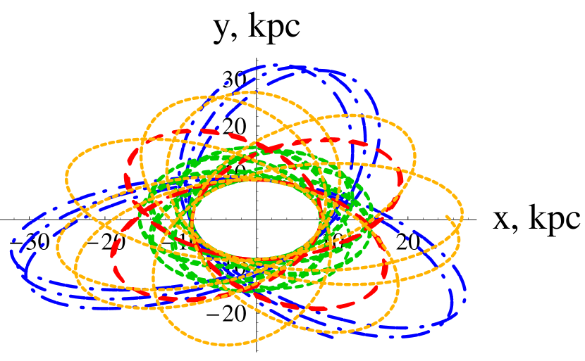
Figure 1: Section in the $\{x,y\}$ plane of the numerically integrated trajectories of the Sun for a) CDM logarithmic halo (dash-dotted blue line) b) CDM NFW halo (dotted yellow line) c) MOND with $\mu=X/(1+X)$ (dashed green line) c) MOG (dashed red line). The time span is $-4.5$ Gyr $\leq t\leq 0$. The initial conditions are those of Table 5 with ([Reid et al. 2009]) $\Theta_{0}=268$ km s^-1.

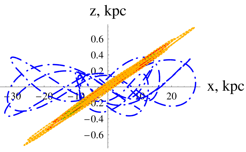
Figure 2: Section in the $\{x,z\}$ plane of the numerically integrated trajectories of the Sun for a) CDM logarithmic halo (dash-dotted blue line) b) CDM NFW halo (dotted yellow line) c) MOND with $\mu=X/(1+X)$ (dashed green line) c) MOG (dashed red line). The time span is $-4.5$ Gyr $\leq t\leq 0$. The initial conditions are those of Table 5 with ([Reid et al. 2009]) $\Theta_{0}=268$ km s^-1.

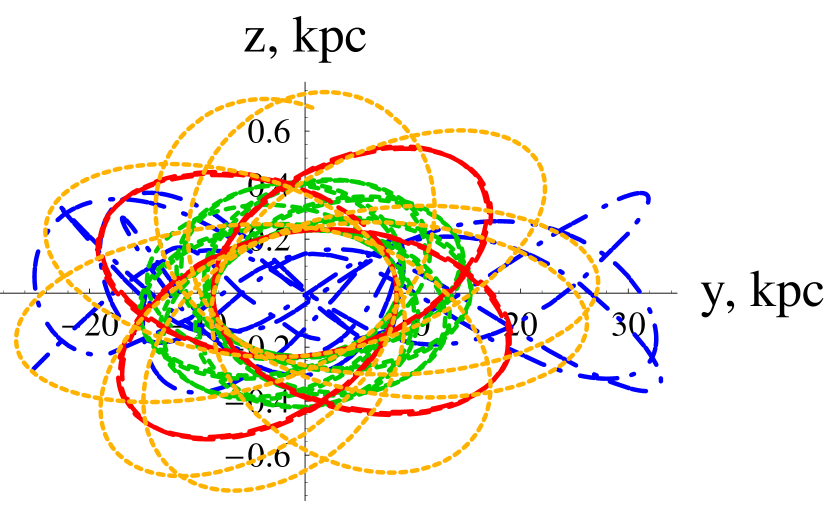
Figure 3: Section in the $\{y,z\}$ plane of the numerically integrated trajectories of the Sun for a) CDM logarithmic halo (dash-dotted blue line) b) CDM NFW halo (dotted yellow line) c) MOND with $\mu=X/(1+X)$ (dashed green line) c) MOG (dashed red line). The time span is $-4.5$ Gyr $\leq t\leq 0$. The initial conditions are those of Table 5 with ([Reid et al. 2009]) $\Theta_{0}=268$ km s^-1.

The orbital trajectories of the Sun are quite different in CDM, MOND and MOG; the largest spatial extension occur for the CDM models, especially for the one characterized by the CDM logarithmic halo The Galactocentric coordinates and distances of the Sun at $t=-4.5$ Gyr are quoted in Table 6.

Table 6: Galactocentric coordinates and distance of the Sun at $t=-4.5$ Gyr according to our numerical integrations of the equations of motion in CDM (logarithmic halo), CDM (NFW halo), MOND and MOG for ([Reid et al. 2009]) $\Theta_{0}=268$ km s^-2. The initial conditions of Table 5 have been used.

Model	$x$	$y$	$z$	$r$
	(kpc)	(kpc)	(kpc)	(kpc)
CDM log	$9.9$	$-25.2$	$-0.3$	$27.1$
CDM NFW	$25.1$	$0.7$	$0.7$	$25.1$
MOND $\left(\mu=\frac{X}{1+X}\right)$	$4.4$	$11.1$	$0.1$	$12.0$
MOG	$15.4$	$-3$	$0.4$	$15.7$

It can be noted that the models considered place the birth of the Sun from a minimum of 12.0 kpc (MOND) to a maximum of $25-27$ kpc (CDM) from GC. This may pose problems concerning the birth of the Earth itself and the development of complex life on it because of, e.g., the presumable low level of metallicity (the amount of elements heavier than hydrogen and helium) in so distant regions. For a discussion and the implications of the concept of Galactic Habitable Zone (GHZ), see [Lineweaver et al. (2004)], [Gonalez (2005)] and [Prantzos (2008)]. In particular, see Figure 5 by [Prantzos (2008)] which shows that the probability of having Earths formed 4 and 8 Gyr after the formation of MW, which roughly corresponds to the birth of the Sun by assuming a Milky Way age of about $10-12$ Gyr, is practically null at Galactocentric distances larger than $10-15$ kpc.

In Figure 4-Figure 6 we repeat the same integrations by using the IAU recommended value $\Theta_{0}=220$ km s^-1.

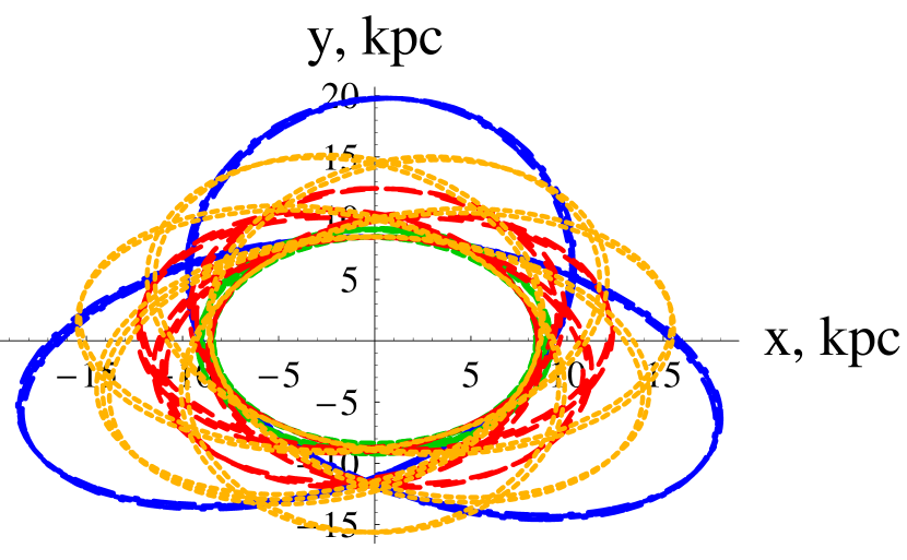
Figure 4: Section in the $\{x,y\}$ plane of the numerically integrated trajectories of the Sun for a) CDM logarithmic halo (dash-dotted blue line) b) CDM NFW halo (dotted yellow line) c) MOND with $\mu=X/(1+X)$ (dashed green line) c) MOG (dashed red line). The time span is $-4.5$ Gyr $\leq t\leq 0$. The initial conditions are those of Table 5 with the IAU recommended value $\Theta_{0}=220$ km s^-1.

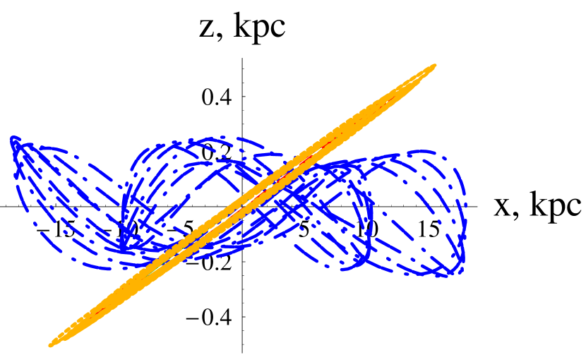
Figure 5: Section in the $\{x,z\}$ plane of the numerically integrated trajectories of the Sun for a) CDM logarithmic halo (dash-dotted blue line) b) CDM NFW halo (dotted yellow line) c) MOND with $\mu=X/(1+X)$ (dashed green line) c) MOG (dashed red line). The time span is $-4.5$ Gyr $\leq t\leq 0$. The initial conditions are those of Table 5 with the IAU recommended value $\Theta_{0}=220$ km s^-1.

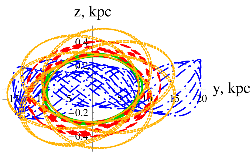
Figure 6: Section in the $\{y,z\}$ plane of the numerically integrated trajectories of the Sun for a) CDM logarithmic halo (dash-dotted blue line) b) CDM NFW halo (dotted yellow line) c) MOND with $\mu=X/(1+X)$ (dashed green line) c) MOG (dashed red line). The time span is $-4.5$ Gyr $\leq t\leq 0$. The initial conditions are those of Table 5 with the IAU recommended value $\Theta_{0}=220$ km s^-1.

The Galactocentric coordinates and distances of the Sun at $t=-4.5$ Gyr for $\Theta_{0}=220$ km s^-1 are quoted in Table 7.

Table 7: Galactocentric coordinates and distance of the Sun at $t=-4.5$ Gyr according to our numerical integrations of the equations of motion in CDM (logarithmic halo), CDM (NFW halo), MOND and MOG. The initial conditions of Table 5 have been used with the IAU recommended value $\Theta_{0}=220$ km s^-2.

Model	$x$	$y$	$z$	$r$
	(kpc)	(kpc)	(kpc)	(kpc)
CDM log	$-18.1$	$-4.7$	$0.1$	$18.8$
CDM NFW	$7.1$	$-5.2$	$0.2$	$8.8$
MOND $\left(\mu=\frac{X}{1+X}\right)$	$6.1$	$6.5$	$0.2$	$8.9$
MOG	$9.2$	$1.1$	$0.3$	$9.3$

Now the situation is quite different because, apart from the logarithmic CDM halo, all the other models locate the birth of the Sun at $8.8-9.3$ kpc from GC

4 Summary and Conclusions

By using the latest kinematical determinations of the full 3D solar motion in the Milky Way, implying a LSR rotation of $\Theta_{0}=268$ km s^-1, we used them as initial conditions for numerically integrating the equations of motion of the Sun backward in time ($-4.5$ Gyr $\leq t\leq 0$) in Newtonian mechanics with two models for the CDM halo, in MOND and in MOG. As a result, the orbital trajectories are not circular and differ each other, with the CDM models yielding the widest spatial extensions of the Sun’s orbit. It turns out that for $t=-4.5$ Gyr the Sun is at quite large Galactocentric distances ($r\approx 12-27$ kpc depending on the models). Instead, by using the standard IAU value $\Theta_{0}=220$ km s^-1 the situation is different: the orbits are less wide and at $t=-4.5$ Gyr the Sun is at $8.8-9.3$ kpc from GC for almost all the models considered.