Simulated SKA maps from Galactic 3D-emission models

Abstract

Context. Planning of the Square Kilometre Array (SKA) requires simulations of the expected sky emission at arcsec angular resolution to evaluate its scientific potential, to constrain its technical realization in the best possible way and to guide the observing strategy.

Aims. We simulate high-resolution total intensity, polarization and rotation measure (RM) maps of selected fields based on our recent global 3D-model of Galactic emission.

Methods. Simulations of diffuse Galactic emission are conducted using the hammurabi code modified for arcsec angular resolution patches towards various Galactic directions. The random magnetic field components are set to follow a Kolmogorov-like power law spectrum.

Results. We present maps for various Galactic longitudes and latitudes at 1.4 GHz, which is the frequency where deep SKA surveys are proposed. The maps are about $1\aas@@fstack{\circ}5$ in size and have an angular resolution of about $1\aas@@fstack{\prime\prime}6$. We analyse the maps in terms of their probability density functions (PDFs) and structure functions. Total intensity emission is more smooth in the plane than at high latitudes due to the different contributions from the regular and random magnetic field. The high latitude fields show more extended polarized emission and RM structures than those in the plane, where patchy emission structures on very small scales dominate. The RM PDFs in the plane are close to Gaussians, but clearly deviate from that at high latitudes. The RM structure functions show smaller amplitudes and steeper slopes towards high latitudes. These results emerge from the fact that much more turbulent cells are passed through by the line-of-sights in the plane. Although the simulated random magnetic field components distribute in 3D, the magnetic field spectrum extracted from the structure functions of RMs conforms to 2D in the plane and approaches 3D at high latitudes. This is partly related to the outer scale of the turbulent magnetic field, but mainly to the different lengths of the line-of-sights.

Conclusions. The significant scatter of the simulated RM distributions agrees with the large scatter of observed RMs of pulsars and extragalactic sources in the Galactic plane and also at high Galactic latitudes. A very dense grid of RMs from extragalactic sources is required to trace and separate Galactic RM foreground fluctuations. Even at high latitudes total intensity and polarized emission is highly structured, which will contaminate sensitive high-resolution extragalactic observations with the SKA and have to be separated in an appropriate way.

1 Introduction

Intensive radio emission from the Galaxy originates from ionized thermal gas, cosmic rays and magnetic fields. All-sky surveys yield an overview of the Galactic structures. However, to reveal distributions of the Galactic emission components, modelling is required because of our position inside the Galaxy. Galactic emission is a severe foreground contamination for observations of fluctuations of the cosmic microwave background radiation and of all kinds of distant, faint extragalactic objects, which will be investigated by the Square Kilometre Array (SKA) with unprecedented sensitivity. Therefore it is crucial to properly account for Galactic emission in all directions of the sky. Unfortunately, most of the properties of the aforementioned constituents of the Galaxy from large scales to small scales are insufficiently constrained up to now.

The large-scale Galactic magnetic field is of particular interest. It has been intensively studied by using rotation measures (RMs) of pulsars (e.g. Han et al., 2006; Noutsos et al., 2008) and extragalactic sources (EGSs) in the Galactic plane (e.g. Brown et al., 2003, 2007). Pulsar dispersion measures (DMs) are used to find their distances based on a thermal gas distribution model. Recent pulsar results indicate a number of magnetic field reversals within the Galaxy (e.g. Han et al., 2006; Noutsos et al., 2008), which is difficult to understand in terms of a simple axi-symmetric or bi-symmetric magnetic field configuration. A more dense RM grid is needed to derive a clear large-scale pattern, because complications arise from local magnetic field disturbances or excessive thermal gas contributions to the observed pulsar DMs and RMs (Mitra et al., 2003). Such effects must be separated to derive a reliable large-scale magnetic field configuration. Moreover, to decompose the observed RM information into a magnetic field contribution, a detailed knowledge of the thermal gas distribution is required. The currently widely accepted distribution of Galactic diffuse thermal gas, the NE2001 model, as well as its filling factor modelled from pulsar and H$\alpha$ observations was presented by Cordes & Lazio (2002) and Berkhuijsen et al. (2006), respectively. Galactic magnetic field models based on pulsar RM observations have to agree with the observed RMs of extragalactic sources shining through the entire Galaxy. To establish a firm picture of the large-scale magnetic field needs to account for all the effects above.

Recently, Sun et al. (2008) have derived a Galactic 3D-emission model which reproduces all-sky surveys over a wide frequency range and also the all-sky RM distribution of EGSs. The simulated maps have an angular resolution of about 15$\arcmin$, which is suitable to compare them with all-sky maps having lower angular resolution. Based on these global results for the Galaxy, simulated arcsec angular resolution maps are the next step in order to get an idea what might be observed with the SKA and other future high-resolution radio telescopes. It is important to understand the origin of the observed structures at high angular resolution to estimate the contamination of extragalactic observations by Galactic small-scale structures as the foreground.

One of the key science projects for the SKA is “Cosmic Magnetism”, where RMs of about $2\times 10^{7}$ polarized EGSs are proposed to be observed in a region of $10^{4}$ deg² (Beck & Gaensler, 2004). The survey is proposed for 1.4 GHz with a resolution of about $1\arcsec$. Simulations of the expected number density of faint sources and their polarization properties from SKA observations were made by e.g. Wilman et al. (2008). A feasibility study on the decomposition of the source RMs from the Galactic foreground RMs and its removal need high-resolution Galactic RM maps. This is the basic motivation for extending our simulations to selected Galactic patches with arcsec angular resolution.

Fluctuations of the components of the interstellar medium (ISM) dominate the emission structures at high angular resolution. The thermal electron density distribution has been found to follow a Kolmogorov-like power law from about $10^{8}$ m to about $10^{18}$ m (Armstrong et al., 1995). The fluctuations of the Galactic magnetic field are mainly studied based on the analysis of the structure function of RMs, where an additional effort is needed to decouple the magnetic field and the electron density fluctuations (Minter & Spangler, 1996). The outer scale of turbulence was reported to be in the range of about 100 pc (Armstrong et al., 1995; Haverkorn et al., 2008) down to a few pc (Minter & Spangler, 1996; Haverkorn et al., 2008).

We summarize our global Galactic 3D-modelling in Sect. 2. The high angular resolution simulation method and the treatment of small-scale magnetic fields are described in Sect. 3. Results and analysis of the simulated RM maps are presented in Sect. 4, including a discussion of the consequences of the simulated RM fluctuations. In Sect. 5 we discuss the results of the simulated total intensity and polarization maps. Some general conclusions are given in Sect. 6.

2 A new Galactic 3D-emission model

Sun et al. (2008) presented a new Galactic 3D-emission model, which is in agreement with a wide range of observations:

• Galactic synchrotron radiation being best represented by the 408 MHz all-sky survey (Haslam et al., 1982) in total intensity and by the WMAP 22.8 GHz all-sky survey in polarized intensity (Page et al., 2007).

• Optically thin thermal emission by the WMAP 22.8 GHz free-free emission template (Hinshaw et al., 2007), and optically thick thermal emission causing absorption, which reflects in a spectral flattening at low frequencies along the Galactic plane.

• The all-sky 1420 MHz polarization survey combined from northern (Wolleben et al., 2006) and southern sky data (Testori et al., 2008) constraining depolarization properties of the interstellar medium.

• RM data from EGSs along the Galactic plane taken from the Canadian (CGPS) and the Southern Galactic Plane Survey (SGPS) (Brown et al., 2003, 2007), and EGSs out of the plane from Han et al. (1999), including preliminary RMs from the new Effelsberg L-band survey (Han et al., in prep.), and RMs from the CGPS high latitude extension (Brown et al., in prep.).

The Galactic 3D-model is based on the 3D-distribution of thermal electrons in the Galaxy (NE2001 model) derived from pulsar DMs by Cordes & Lazio (2002). To successfully model the observed thermal emission for the optically thin case and absorption effects from the optically thick gas, the filling factor of thermal gas needs to be taken into account, whose spatial variation was derived by Berkhuijsen et al. (2006). The regular Galactic disk magnetic field model was constrained by extragalactic RM data of Brown et al. (2003, 2007). Axi-symmetric (ASS) and bi-symmetric (BSS) fields with one field reversal inside the solar circle agree with extragalactic RM data in the plane, while the BSS field configuration fails to represent the RM gradient with Galactic latitude as measured from the high-latitude extension of the CGPS by Brown et al. (in prep.). The 408 MHz survey (Haslam et al., 1982) and the WMAP 22.8 GHz linear polarization survey (Page et al., 2007) were used to constrain the random magnetic field component, the cosmic-ray electron distribution, and the known local synchrotron excess. Finally, the depolarization effects of the 1420 MHz polarization survey (Wolleben et al., 2006; Testori et al., 2008) were modelled, which requires to modify the thermal filling factor by adding an extra coupling term of the electron density and the random magnetic field.

The quantitative model parameters of the three constituents of the Galaxy are those of the NE2001 thermal electron density model, an ASS magnetic field configuration with a local strength of 2 $\mu$G, asymmetric toroidal halo fields with respect to the plane with a maximum strength of 10 $\mu$G, isotropic and homogeneous random magnetic fields with a strength of 3 $\mu$G, and a cosmic-ray electron distribution truncated at 1 kpc above and below the plane. The details are given by Sun et al. (2008).

Although this Galactic 3D-model is in agreement with the observed all-sky maps, some of its parameters seem unrealistic. To fit the observed high-latitude RMs, a strong regular halo magnetic field is required, because the scale height of the thermal electrons of the NE2001 model is just about 1 kpc. The strong halo field in turn requires a cosmic-ray electron distribution limit of about 1 kpc to avoid excessive high-latitude synchrotron emission. These parameters are unrealistic for both the halo field strength (Moss & Sokoloff, 2008) and the distribution of cosmic-ray electrons. Sun et al. (2008) note that by increasing the scale height of the thermal electron density to about 2 kpc the halo magnetic field strength reduces to about 2 $\mu$G and the truncation of the cosmic-ray distribution turns obsolete. Recently, Gaensler et al. (2008) critically reanalyzed the thermal electron scale height and quote a revised value of 1.8 kpc, very close to the proposed 2 kpc by Sun et al. (2008). This makes the Galactic properties similar to those observed for nearby galaxies. It should be noted that the simulated maps are not affected by these modifications of parameters.

3 High-resolution simulations

3.1 The general simulation concept

The simulations presented in this paper make use of the hammurabi code (Waelkens, 2005; Waelkens et al., 2009), where the sky is pixelized according to the HEALPix scheme (Górski et al., 2005). Each pixel contains information from a cone shaped volume centered at the observer. Each surface element is quadrilateral and covers the same area. The number of pixels $N_{\rm pix}$ of a sphere are calculated by $N_{\rm pix}=12N^{2}_{\rm SIDE}$, where $N_{\rm SIDE}$ is an integer power of 2. Therefore d$\Theta$, the linear size or the angular resolution, can be calculated as

$${\rm d}\Theta=\sqrt{\frac{3}{\pi}}\frac{3600\arcmin}{N_{\rm SIDE}}.$$ (1)

For each pixel of the map, the Stokes parameters ($I$, $U$ and $Q$) and the RM are integrated in the radial direction from the observer up to a maximal distance $r_{\rm max}$ (Sun et al., 2008). The modelled emission distributions in the Galaxy are represented in cylindrical coordinates with the origin at the Galactic center. The distance to the Sun is taken as 8.5 kpc. Details of the regular magnetic field component, the cosmic-ray density and the thermal gas distributions in the disk and halo of the Galaxy are described by Sun et al. (2008). The integration process samples these distributions and inherently accounts for depolarization. To accurately calculate the integral, each pixel is separated into many volume units with equal radial interval $\Delta r$. Thus the size of a unit can be approximated as $r{\rm d}\Theta\times r{\rm d}\Theta\times\Delta r$ with $r$ being the distance of the volume unit to the observer. This process is repeated for all pixels, which are finally combined to an all-sky map.

3.2 Zoom-in for specified patches

According to Eq. (1) the possible resolutions depend on $N_{\rm SIDE}$. To achieve arcsec resolution and to optimize the amount of computation time, we use $N_{\rm SIDE}$ of 131072, which corresponds to a resolution of about $1\aas@@fstack{\prime\prime}6$. The pixel number for an all-sky map then amounts to about $2\times 10^{11}$, which is far beyond any computer memory capacity today. Therefore high-resolution simulations are just possible for a small patch of sky. Thus we adapted the hammurabi code to be able to simulate parts of the sky.

In the hammurabi code the NEST ordering (Górski et al., 2005) is used, which facilitates the zoom-in of specified patches as it is explained below. For $N_{\rm SIDE}=1$ the entire sky is split into 12 patches as shown in Fig. 1. They are numbered from 0 to 11. For $N_{\rm SIDE}=2$, each pixel is further split into four child pixels, also shown in Fig. 1 for patch “5”. This patch is centered at longitude of $90\degr$ in the plane with a diagonal size of about $90\degr\times 90\degr$. Subsequently for $N_{\rm SIDE}$ increasing by 2 each pixel is further split into four pixels. In this scheme one can determine a target patch and make proper splits depending on the resolution. To reach a smaller patch size and higher angular resolution a much larger value for $N_{\rm SIDE}$ is required.

Figure 1: The HEALPix pixel scheme (Górski et al., 2005) for Galactic coordinates used in this paper.

3.3 Realization of the random magnetic field component

It is generally accepted that the power spectrum of the random magnetic field component should follow a power law as $P(k)\propto k^{\alpha}$. Here $k=2\pi/l$ is the wave vector and $l$ is the spatial scale. For a Kolmogorov-like turbulence spectrum the spectral index is $\alpha=-11/3$, which is used in all present simulations. Note that independent fluctuations of the electron density are not included in the simulations. Howver, fluctuations of the electron density are also expected to follow a Kolmogorov-like spectrum (Armstrong et al., 1995). The coupling of electron density and random magnetic fields we introduced in our all-sky simulations to model the observed depolarization (Sun et al., 2008) results in Kolmogorov-like fluctuations for both components.

Random magnetic field components realized in the simulations presented by Sun et al. (2008) are generated in situ for every volume unit by Gaussian random numbers. To obtain the random magnetic field components following a given power-law spectrum, an inverse Fourier transformation must be performed. All available fast Fourier transformation (FFT) algorithms are based on a Cartesian coordinate system. We therefore set-up a cubic box with a size of $L^{3}$ and divide it into $N^{3}$ small cubes with a common volume of $\Delta^{3}$. Within the box we construct a Cartesian coordinate system and perform the FFT to derive the random field strength and direction in each small cube. Here $L$ corresponds to the outer scale of the turbulence and $\Delta$ corresponds to the inner scale.

An important constraint for $\Delta$ is that $\Delta\leq r{\rm d}\Theta$. This ensures that several neighbouring line-of-sights do not pass the same small cubes. Otherwise spurious stripes are seen in the maps. For $r$ of about 1 kpc and ${\rm d}\Theta$ of $1\aas@@fstack{\prime\prime}6$ the size of a small cube should not be larger than about 0.01 pc. If our Galaxy is treated as one box, meaning $L=40$ kpc, the total number of cubes is about $6.4\times 10^{19}$. Again there is no way in processing this huge amount of cubes by current computing facilities.

In our simulation, we devise a scheme to generate the random magnetic field components in an adequate way. We first conduct a FFT to create a magnetic field distribution in a box. We then rotate this box to acquire new boxes, which are glued together to fill the entire Galaxy. The box rotation angles are integer multiples of $\pi/2$, which avoids cutting of boxes. Through this scheme the turbulence status of the Galaxy is realized. This process is detailed in Appendix A.

Actually the size of the box cannot be too small, otherwise there are too many boxes to handle. On the other hand $L$ cannot be too large in order to get a reasonable number of cubes of about 0.01 pc in size. As a compromise, we take a size of 10 pc for the box and of 0.0125 pc for the cubes. Although 0.0125 pc is much larger than the inner scale of the electron density fluctuations, which are of the order of $10^{8}$ cm (e.g. Armstrong et al., 1995), it is sufficient for our study in regard to the current angular resolution. In total there are about $5\times 10^{8}$ cubes, requiring a memory of about 12 giga-byte for the random magnetic field components when stored as double precision numbers. It is thus obvious that the number of cubes is a compromise between high resolution, which requires small cube sizes, and hence a very large number of cubes and the available computer memory, which is thus able to handle a limited number of cubes.

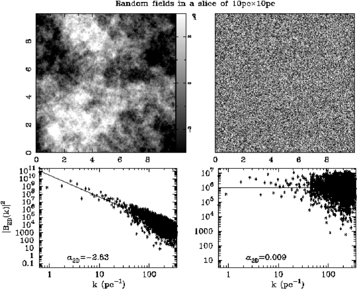
Figure 2: 2D random magnetic field distribution in a slice parallel to one surface of a 10 pc box. The upper left panel shows magnetic field components following a power law index of $-11/3$, while the upper right panel shows random field components realized by random Gaussian numbers corresponding to a spectral index of zero. Their corresponding power spectra are shown in the lower panels.

In Fig. 2, we show the 2D-distribution of random magnetic field components for a slice parallel to one surface of a 10 pc box. For comparison, we show the random magnetic fields generated in situ in each grid of the same plane as random Gaussian number, which is similar to that used by Sun et al. (2008). The power spectra of the magnetic fields are also shown in Fig. 2. It is apparent that the distribution of random magnetic fields following a power-law spectrum shows coherent structures of various extent, whereas the Gaussian random magnetic field distribution is featureless. The spectral index of $\alpha_{\rm 2D}=-2.83\approx\alpha+1$ for Kolomogorov magnetic field distributions and $\alpha_{\rm 2D}=0$ for Gaussian field distributions agree with the expectations and prove that the random magnetic field components are properly distributed in the box.

4 Modelling results on rotation measures

Except for the random magnetic fields the simulations presented below use the same Galactic 3D-emission models as derived by Sun et al. (2008), where the “ASS+RING” model for the disk magnetic field is selected here. The random magnetic fields are introduced as described above and follow a Kolmogorov-like spectrum. The strength of the random fields is scaled to 3 $\mu$G which is the same as that in Sun et al. (2008). All simulations are made for 1.4 GHz observations, as this is the proposed SKA RM survey frequency. As mentioned above, the simulated patch size is limited by available computer memory, so that just relatively small patches of about $1\aas@@fstack{\circ}5$ in size are simulated at a resolution of $1\aas@@fstack{\prime\prime}6$. This is compatible with the expected SKA angular resolution.

Simulations are presented for a handful of patches only, because each run takes very long computation time. We select the first patch around $(l,\,\,b)\,=\,(135\degr,\,\,+40\degr)$, which is in the direction of the DRAO Planck Deep Fields (Taylor et al., 2007), where soon high-resolution continuum and polarization data will be available. This patch is named MN standing for Medium-latitude-North. More patches with roughly the same longitude, but with different latitudes, are further selected. These are labeled HN (High-latitude-North), PNAC1 (Plane-North-Anti-Centre 1), PSAC (Plane-South-Anti-Centre), MS (Medium-latitude-South) and HS (High-latitude-South). To compare with PNAC1, three additional patches in the plane, PNAC2 (Plane-North-Anti-Centre 2), PNC1 and PNC2 (Plane-North-Centre 1 and 2) are included. The centre coordinates of these patches are listed in Table 1. Note that we cannot set the patch coordinates to exactly the same longitudes or latitudes because of HEALPix constraints (Górski et al., 2005). In Table 1 also the maximal integral lengths or the length of line-of-sights ($r_{\rm max}$) and the integral steps ($\Delta r$) are listed. The integral length is determined by taking into account the cosmic-ray scale height of about 1 kpc and the disk cutoff radius of 17.5 kpc for the electron density in the NE2001 model (Cordes & Lazio, 2002). Integrating further out results in negligible contributions. For the patches with large integral length, the step size is larger than for those with small length to limit the computation time. The selected patches allow to study variations of emission and RM structures related to turbulent magnetic field components versus Galactic longitudes and latitudes. Variations of the structure functions for RMs from EGSs as a function of Galactic direction have already been noted by Sun & Han (2004) for angular scales of several degrees.

Table 1: Simulated patches.

name	$l$ ($\degr$)	$b$ ($\degr$)	$r_{\rm max}$ (kpc)	$\Delta r$ (pc)
HN	138.33	70.16	3	1.0
MN	136.48	44.20	3.5	1.0
PNAC1	130.07	1.19	10	2.5
PSAC	130.07	$-$1.19	10	2.5
MS	136.48	$-$44.20	3.5	1.0
HS	138.33	$-$70.16	3	1.0
PNC1	59.77	1.19	30	3.8
PNC2	300.23	1.19	30	3.8
PNAC2	229.92	1.19	10	2.5

All simulations were made by using the computer cluster of the Max-Planck-Institut für Radioastronomie operated by the VLBI group.

4.1 Overview of the results

As described by Sun et al. (2008) the hammurabi simulations result in Stokes $I$, $U$, and $Q$ maps at the specified frequency as well as the RM maps. Subsequently, the polarization angle ($PA$) and polarized intensity ($PI$) maps are calculated according to $PA=\frac{1}{2}{\rm atan}\frac{U}{Q}$ and $PI=\sqrt{U^{2}+Q^{2}}$.

In this paper, we will not discuss the separation process of total and polarized intensities of EGSs from the foreground, which requires adding polarized EGSs and noise to the simulated maps. The simulated RMs represent the contribution of the whole Galaxy to the RM from an EGS in case the source size does not exceed the pixel size of the simulated map. Thus, the RM maps are directly related to observations. Below we focus on the analysis of RM maps, which are directly connected to the planned SKA RM survey. All simulated RM maps are shown in Fig. 3. The other maps are shown in Figs. 11, 12, 13, 14, and 15 in Appendix B.

The RM maps clearly show structures ranging from small to large scales. The variation of the structures versus latitudes is also evident. Below some statistical methods are applied to analyse these structures.

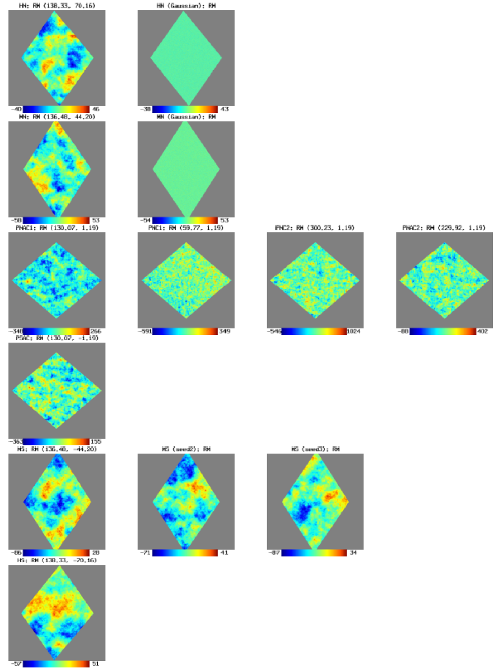
Figure 3: RM maps for all simulated patches ordered from high to low latitudes (top to bottom) in gnonomic projection. Their designation and Galactic coordinates are quoted on top of each individual panel (also listed in Table 1). Different simulations for the same patch and for patches at the same latitude, but different longitudes, are shown in one row (see text for details). Each field has about $3000\times 3000$ pixel and a size of about $1\aas@@fstack{\circ}5\times 1\aas@@fstack{\circ}5$. The minimum and maximum of each map is shown together with the wedge below each panel.

4.2 Statistical description of the simulations

The rotation measure, RM, is defined as

$${\rm RM}=K\int_{0}^{r_{\rm max}}n_{e}(B_{\parallel}+b_{\parallel}){\rm d}r,$$ (2)

where $K$ is a constant, $n_{e}$ is the thermal electron density, $B_{\parallel}$ and $b_{\parallel}$ are the regular and random magnetic field components projected along the line-of-sight, respectively, and $r_{\rm max}$ is the maximal distance along the line-of-sight from the observer. One major question is to what extent the properties of $B$ and $b$ can be recovered from the RM maps.

4.2.1 The probability distribution function

We use the probability distribution function (PDF) to describe the structure properties of a map as discussed by Mizeva et al. (2007). For the RM distribution $\rm{PDF}\leavevmode\nobreak\ ({\rm RM})\times\Delta{\rm RM}$ quantifies the relative number of pixels falling between ${\rm RM}$ and ${\rm RM}+\Delta{\rm RM}$. A Gaussian shape of the PDF indicates that no extended features are present in the map. To measure the deviation from a Gaussian distribution, two more parameters, skewness and kurtosis, are used (e.g. Kowal et al., 2007),

$$\begin{array}[]{rcl}{\rm skewness}&=&\displaystyle{\frac{1}{N}\sum_{i=1}^{N}\left(\frac{{\rm RM}_{i}-\overline{\rm RM}}{\sigma_{\rm RM}}\right)^{3}}\\[14.22636pt] {\rm kurtosis}&=&\displaystyle{\frac{1}{N}\sum_{i=1}^{N}\left(\frac{{\rm RM}_{i}-\overline{\rm RM}}{\sigma_{\rm RM}}\right)^{4}-3},\end{array}$$ (3)

where $\overline{\rm RM}$ and $\sigma_{\rm RM}$ are the average and standard variance of the RM maps. They are third and fourth order statistical moments, respectively. Large absolute values of skewness or kurtosis indicate that either the tail or the centre of the Gaussian is deformed. Physically these parameters are closely related to turbulence properties (Kowal et al., 2007).

The RM PDFs for all simulated patched are shown in Figs. 4, 6, 7, and 8 (upper panels). Their average values, together with variance, skewness and kurtosis are listed in Table 2.

Table 2: Statistical parameters for the simulated RM patches. The patch designations are listed in Table 1. Note that for the patches HN, MN and MS more realizations were made with details given in the text.

name	average	variance	skewness	kurtosis
	(rad m-2)	(rad m-2)
HN	2.50	12.73	0.0857	$-$0.2555
HN (Gaussian)	2.14	8.11	$-$0.0007	0.0008
MN	$-$1.90	15.12	0.0347	$-$0.2287
MN (Gaussian)	1.41	10.93	$-$0.0007	0.0009
PNAC1	$-$85.82	63.40	0.0654	0.2124
PSAC	$-$103.13	60.86	$-$0.0482	$-$0.0274
MS (seed1)	$-$27.58	18.81	$-$0.1464	$-$0.6365
MS (seed2)	$-$19.78	16.74	0.1338	$-$0.2968
MS (seed3)	$-$24.86	16.35	$-$0.1847	0.3896
HS	1.66	17.15	$-$0.1241	$-$0.6353
PNC1	$-$89.03	93.65	$-$0.0018	0.0646
PNC2	286.53	155.71	$-$0.0045	0.0528
PNAC2	159.80	50.80	0.0217	$-$0.0429

4.2.2 The structure function

For turbulence studies, it is customary to investigate the power spectrum of the magnetic field, which can be retrieved from the power spectrum, autocorrelation function, or structure function of RMs (e.g. Simonetti et al., 1984; Minter & Spangler, 1996; Enßlin & Vogt, 2003). Observationally always uneven sampled RMs of EGSs are obtained. In this case the structure function is suited best (Sun & Han, 2004). Since RM maps are available as simulation results, the autocorrelation function is also investigated here as a crosscheck for the structure function results. The structure function ($D_{\rm RM}(\delta\theta)$) is defined as

$$D_{\rm RM}(\delta\theta)=\frac{[{\rm RM}(\@vec{\theta})-{\rm}RM(\@vec{\theta+\delta\theta})]^{2}}{N_{\rm pairs}},$$ (4)

where $\delta\theta$ is the angular separation of two pixels and $N_{\rm pairs}$ is the number of RM pairs with the same angular separation.

It would take a huge amount of computing time to obtain the structure functions from all pixels of our simulated maps. We simplified this by randomly selecting $N_{s}$ pixels to conduct the calculation for structure functions. These pixels are randomly distributed across the maps. To accurately assess the structure functions for small angular separations, the number $N_{s}$ should be as large as possible. As a compromise we selected $N_{s}=2\times 10^{5}$ pixels from the maps. The structure functions are shown in Figs. 4, 6, 7 and 8 (lower panels).

Table 3: Fitting results for structure functions and autocorrelation functions of RMs.

	structure functions				autocorrelation function
name	$A$	$\Delta A$	$m$	$\Delta m$	$B$	$\Delta B$	$s$	$\Delta s$
HN	34.8	0.4	0.916	0.006	8.6	0.1	0.957	0.008
MN	62.7	0.2	0.862	0.002	15.7	0.2	0.853	0.010
PNAC1	2951.1	29.9	0.719	0.007	596.0	3.9	0.773	0.013
PSAC	2830.4	11.6	0.751	0.002	596.8	5.9	0.831	0.017
MS	64.9	0.5	0.871	0.005	24.5	0.4	0.915	0.010
HS	42.0	0.4	0.909	0.005	11.5	0.1	0.913	0.006
PNC1	13695.7	293.8	0.658	0.010	2255.7	16.4	0.614	0.018
PNC2	31230.9	402.2	0.676	0.008	5792.6	40.0	0.661	0.013
PNAC2	2836.0	57.4	0.660	0.013	738.3	5.5	0.743	0.014

The theoretical deduction how structure functions are related to the power spectrum of magnetic fields has been given by Minter & Spangler (1996), where the structure function of RMs is found to follow a power law as $D_{\rm RM}(\delta\theta)=A\delta\theta^{m}$ with $A$ being a constant and the spectral index $m$ being related to the power low index $\alpha$ of $P(k)$ as $m=-\alpha-2$. This relation holds for the inertial range, i.e., for the scale $l_{\rm i}<l<l_{\rm o}$, where $l_{\rm i}$ and $l_{\rm o}$ are inner and outer scales, respectively. The angular inertial scale can thus be defined as $\delta\theta_{\rm i}<\delta\theta<\delta\theta_{\rm o}$, where $\delta\theta_{\rm i}=l_{\rm i}/r_{\rm max}$ and $\delta\theta_{\rm o}=l_{\rm o}/r_{\rm max}$. In principle the inertial range can be estimated by checking where the linear fit of the structure functions for a logarithmic scale fails. For the structure functions from our simulated results, we are able to infer the outer scale but the inner scale is smaller than the pixel size. Below we name the outer angular scale $\delta\theta_{\rm o}$ as the transition angle. The fit results for structure functions are listed in Table 3.

Enßlin & Vogt (2003) have noted that the very inner part of the autocorrelation function of RMs ($\xi_{\rm RM}$) can be written as $\xi_{\rm RM}(0)-\xi_{\rm RM}(\delta\theta)=B\delta\theta^{s}$, where $B$ is a constant, and $s=-\alpha-2$ is the spectral index of the magnetic energy spectrum. This implies that the power law index of the structure function $m$ and the power law index of the autocorrelation function $s$ should be equal. We obtain the autocorrelation functions by a Fourier transform of the RM power spectra and show them in Fig. 5. The RM fit results for each patch are listed in Table 3. As can be seen, the spectral indices of the autocorrelation functions do not deviate very much from that of the structure functions. We account the differences mainly to computational effects when obtaining the autocorrelation functions. Unwanted components might be introduced during the pixelization of the maps when Fourier transformed. Therefore we are confident that the results based on the two methods are basically consistent with each other.

Figure 4: PDFs and structure functions of the patches HN and MN at high and medium latitudes. See Tables 1 and 2 for details of the patch parameters.

Figure 5: Autocorrelation functions for RMs.

The spectral index of 5/3 is expected from the power law fit of the RM structure functions for a Kolmogorov-like turbulent magnetic field. This, however, is not seen in Table 3. Possible explanations are discussed in Sect. 4.7.1.

4.3 Gaussian versus Kolmogorov-like random magnetic fields

In the simulations presented by Sun et al. (2008), the random magnetic field components were realized in situ for each volume unit by Gaussian random numbers. The random fields created that way are called ’Gaussian fields’ below. In that scheme, the simulated RMs are totally uncorrelated between the map pixels, which implies that no small-scale structures are expected. When random magnetic fields with a Kolmogorov-like spectrum are generated, as described in Sect. 3.3, a large number of turbulent boxes are placed along the line-of-sight. For arcsec angular resolutions several neighbouring line-of-sights pass the same boxes, which results in extended coherent features in the simulated RM maps.

For the northern patches HN and MN, we also performed simulations with Gaussian random magnetic field component for comparison. Both RM maps are shown in the first two rows in Fig. 3 and prove the above expectations. As seen from Fig. 4, the PDFs of the RM simulations with Gaussian random magnetic fields nicely conform to Gaussian distributions, while the PDFs from the simulations with Kolmogorov-like random magnetic fields do not. Quantitatively this can be verified by the skewness and kurtosis in Table 2, where the values of these two parameters are much larger for Kolmogorov-like magnetic field spectra than Gaussian ones. The structure functions shown in the bottom panel of Fig. 4 as well as the autocorrelation functions in Fig. 5 reinforce the argument. The structure functions for Gaussian random magnetic fields are flat, while the structure functions for a Kolmogorov-like magnetic field spectrum have slopes, which will be discussed below.

4.4 RM patches from different realizations

The RM structures in the present simulations are no predictions for sky emission structures towards the quoted directions, but are just one possible realization of the random magnetic fields following a Kolmogorov-like power law spectrum in context with other model parameters as described before.

We generate the random magnetic field components in the following way. Their amplitudes are determined according to the slope of the power-law spectrum with a spectral index of $-11/3$, and the phase angles are realized by random numbers. The rotation angle of the numerous 10 pc boxes placed along the line-of-sight are also determined from random numbers. These random numbers are actually pseudo random and are initiated by an integer called “seed”. When the random “seed” number is changed, a different realization of the same random magnetic field distribution is obtained.

To check structure variations and structure functions for different realizations, we ran two more simulations for patch MS with different “seed” numbers. The RM maps are displayed in the fifth row of Fig. 3 and show different distributions of RM features as expected. Also the PDFs for the RM maps (Fig. 6) vary considerably, as well as the parameters listed in Table 2. The structure functions of RMs, however, are almost identical as shown in the bottom panel of Fig. 6, except for regions with large angular separations exceeding about $10\arcmin$, where the structure function becomes less accurate due to the decreasing number of selected pixels.

The mean RM for the three realizations of patch MS is between $-$20 rad m^-2 and $-$28 rad m^-2 (Table 2) and the majority of RMs has negative values. However, due to the variance of up to 19 rad m^-2 (Table 2) all three simulations show a number of small extended features in the maps with positive sign. Naively this could be interpreted as reversals of the large-scale magnetic field in case the available number of observed RMs from EGSs is small. However, in contrast with large-scale reversals in the Galactic plane as discussed for instance by Han et al. (2006), the reversals seen here are entirely caused by the distribution of random magnetic fields. For this medium-latitude area, we roughly estimate the probability for picking up a “reversal” to be about 7%. This should be reflected in the distribution of observed RMs of EGSs and will prove the relevance of the simulations and the parameters used.

Figure 6: PDFs and structure functions of the patch MS for the same amplitudes but different realizations of the phases of the random magnetic field components created in a 10 pc box (see text for details).

4.5 Galactic plane RM patches at different longitudes

In this section we investigate RM variations in the plane versus Galactic longitudes. The four simulated patches have latitudes of about $+1\aas@@fstack{\circ}2$. Two of them (PNC1 and PNC2) are in the inner Galaxy direction and the other two (PNAC1 and PNAC2) are in the anti-centre direction (see Table 1).

The visible structures in the maps (the third row in Fig. 3) are less extended compared to those at higher latitudes. There is more fine structure for the inner Galaxy regions than for those in the anti-centre direction. The PDFs of all four simulated patches closely resemble Gaussian shapes (Fig. 7). The inner Galaxy patches PNC1 and PNC2 have smaller skewness values than the anti-centre patches (Table 2), indicating that their PDFs are more close to Gaussian shapes. Note that the skewness and kurtosis for all patches is very small, which indicates that it is impossible to infer whether the turbulence spectrum is Gaussian or Kolmogorov-like based on their PDF. The structure functions as discussed before, however, clearly reveal the properties of the underlying turbulence spectrum. The average RM values are consistent with the RM results obtained by Sun et al. (2008).

As displayed in Fig. 7, all Galactic plane structure functions are well fitted by power laws. Compared to the medium- and high-latitude fields a flattening of the structure functions occurs at smaller angular distances. The fit results for the power laws are listed in Table 3. From the parameters listed in Table 1 we obtain a transition angle of about $1\arcmin$ for PNC1 and PNC2 and about $3\arcmin$ for PNAC1 and PNAC2. Fig. 7 shows instead of a sharp change in the structure function a smooth transition from a linear slope to a flat curve in the logarithmic scale. The turn over of the structure functions ranges from about $1\arcmin$ to $2\arcmin$ for patches PNC1 and PNC2, from $3\arcmin$ to $5\arcmin$ for patch PNAC1, and from $2\arcmin$ to $5\arcmin$ for patch PNAC2, which are roughly consistent with the aforementioned expectations. The spectral indices are consistent with theoretical predictions by Minter & Spangler (1996) for 2D turbulence, which results in a spectral index of about 0.7 for the structure functions. However, our input turbulent magnetic fields are for 3D. The amplitudes of the structure functions increase towards the inner Galaxy regions, which is expected as the line-of-sights pass more turbulent cells or magnetic field boxes than towards the anti-centre or high-latitude direction. The amplitude of the structure function for PNC1 is larger than that for PNC2, which is mainly due to a larger electron density in this direction according to the NE2001 model.

Figure 7: PDFs and structure functions of the five simulated Galactic plane patches (see Table 1 for field parameters).

4.6 RM patches at different latitudes

We finally compare the different results towards different latitudes. The patches HN/HS, MN/MS,and PNAC1/PSAC have longitudes between $130\degr$ and $140\degr$. The latitudes are $\pm 70\degr$, $\pm 44\degr$ and $\pm 1\degr$. For patch MS the “seed1” case is used. The six simulated RM maps are all shown in the first column of Fig. 3. A clear trend for more extended structures for high-latitude regions is clearly seen. The PDFs for the high-latitude regions (HN/HS and MN/MS) all deviate significantly from Gaussian (Fig. 8 and Table 2).

The structure functions derived for the four high-latitude patches are shown in Fig. 8 and for the five plane patches in Fig. 7. All of them have similar properties. The transition angle is calculated to be about $10\arcmin$ for HN/HS and MN/MS regions, which is consistent with the results displayed in Fig. 8. The amplitudes of the structure functions are smaller for the high-latitude patches compared to those in the plane. This can be understood, because the length along the line-of-sight is small compared to that in the Galactic plane. The number of turbulent cells passed by the line-of-sights is smaller and hence is the amplitude of the structure functions. We also note that the slopes of the structure functions increase for the high-latitude patches. These spectral changes will be discussed below.

Figure 8: PDFs and structure functions of four patches (see first column of Fig. 3) at roughly the same Galactic longitude located at medium and high latitudes (see Table 1).

4.7 Discussion of RM simulations

4.7.1 Theoretical structure functions revisited

From the structure functions of simulated RM maps, we found evidence for latitude-dependent variations of their spectral slope, which gets steeper towards high latitudes. The regular magnetic field and the electron density have spatial irregularities, which are of larger scale than the sizes of the patches. Therefore the large-scale magnetic field cannot cause variations of the spectral slopes, but influences the amplitude of the structure functions. The coupling between the electron density and random magnetic fields introduced by Sun et al. (2008) augments the scattering of RMs and hence the amplitude of the structure function rather than changes its spectral index. For the present simulations, the random magnetic field is comparable to the regular magnetic field strength and dominates the regular field towards high-latitude regions. We conclude that all RM structures across the simulated patches are caused by the random magnetic field properties.

Table 4: Fit parameters for structure functions from different simulation settings.

$L=20$ pc, $r_{\rm max}=10$ kpc
$\Delta$ (pc)	$C$	$\Delta C$	$m$	$\Delta m$
0.80	3.304	0.028	0.727	0.044
0.40	3.430	0.021	0.644	0.033
0.20	3.387	0.030	0.760	0.047
0.10	3.414	0.009	0.612	0.014
0.05	3.447	0.018	0.622	0.028
$\Delta=0.5$ pc, $r_{\rm max}=10$ kpc
$L$ (pc)	$C$	$\Delta C$	$m$	$\Delta m$
200	2.830	0.006	1.262	0.006
100	3.045	0.011	1.081	0.015
50	3.201	0.008	0.982	0.010
25	3.401	0.007	0.709	0.012
$\Delta=0.25$ pc, $L=100$ pc
$r_{\rm max}$ (kpc)	$C$	$\Delta C$	$m$	$\Delta m$
0.01	$-$6.270	0.0181	1.660	0.014
0.05	$-$4.243	0.0106	1.413	0.008
0.10	$-$2.689	0.0128	1.668	0.009
0.20	$-$1.742	0.0172	1.355	0.013
0.40	$-$1.206	0.0202	1.689	0.013
0.80	0.368	0.0133	1.282	0.012
1.60	1.630	0.0088	1.330	0.009
3.20	2.711	0.0060	1.154	0.006
6.40	2.970	0.0083	1.151	0.010
10.00	3.083	0.0078	1.081	0.010

The variations versus latitude must be ascribed to geometric effects, which reflects in the integral length ($r{\rm max}$) as listed in Table 1. The size of the magnetic field box ($L$) is fixed in the simulations presented, therefore, the integral length determines the number of turbulent cells or boxes passed by the line-of-sight. For a sufficient large number of cells, the fluctuations along the line-of-sight are averaged out. This results in a spectral slope of $m=-\alpha-3=2/3$ for the structure function. Note that this spectral index was observed and interpreted as a 2D turbulence in the interstellar medium by Minter & Spangler (1996). 2D turbulence is confined to thin sheets or filaments. However, the present simulations are based on a 3D distribution of the turbulent magnetic field components, which have not the shape of sheets or filaments. When the number of cells is small enough so that the integral length is comparable to the outer scale, the structure function tends to have the index of $m=-\alpha-2=5/3$ as derived by (Minter & Spangler, 1996) for 3D Kolmogorov-like turbulence. Therefore we conclude that in the inertial range ($\delta\theta_{\rm i}<\delta\theta<\delta\theta_{\rm o}$) the derived structure functions shall behave like $D_{\rm RM}(\delta\theta)\propto\delta\theta^{m}$ with $2/3<m<5/3$ depending on the number of cells. When the angular separation is larger than the transition angle, the structure function spectrum flattens and $m$ gradually turns to zero.

To prove these arguments we made several simulations for a patch of about $6\degr\times 6\degr$ in the plane with $N_{\rm SIDE}=2048$ corresponding to a resolution of about $1\aas@@fstack{\prime}7$. Although the resolution is much lower than the high-resolution simulations for the patches in Table 1, the dependence of the structure functions should be the same. These simulations can be realized in much smaller computing time than the arcsec resolution simulations. We fit the structure functions by using $\log D_{\rm RM}(\delta\theta)=C+m\log\delta\theta$ and list the results including errors of C and m in Table 4. We first fix the outer scale ($L$) and the integral length and vary the size of the small cubes ($\Delta$). The results in Table 4 show that the size of the small cubes has little influence on the structure function parameter. We then change the outer scale, but keep the size of the small cubes and also the integral length constant. As expected the spectral index of the structure functions tends to be about 0.7 for very small outer scales, which means the number of turbulent cells is large. Finally, we increase the integral length from 10 pc to 10 kpc by using the same values of cube size and outer scale. The spectral index of the structure functions varies between 1.3 and 1.7 until the integral length exceeds about 1600 pc, becoming smaller for larger lengths. These test simulations support our conclusion that the spectral index of the structure function primarily depends on the number of turbulent cells, which is mainly determined by the length of the line-of-sight. Thus, when assessing the turbulent magnetic field properties from the structure functions of RMs, the line-of-sight dependence must be taken into account. In the Galactic plane the integral length is always large, which assures sufficient turbulent cells being passed through by the line-of-sight. Therefore the relation $\alpha=-m-3$ holds in general. Towards higher Galactic latitudes, however, the length of the line-of-sight decreases and hence also the number of turbulent cells decreases. The spectral index of the random fields approaches $\alpha=-m-2$.

4.7.2 Diagnosis of the Galactic foreground

It has been proposed to conduct a very dense RM survey of EGS with the SKA to study magnetic field structures in the Milky Way, in galaxies, in cluster of galaxies and beyond (Beck & Gaensler, 2004). The key issue to achieve relevant information for extragalactic objects is to properly extract and separate the foreground RM contributions from the observations. We have tested the minimum number of pixel needed to calculate the correct structure function for the simulated maps and found that about 10000 pixel are required. For our map size this corresponds to a mean angular separation of about $1\arcmin$ in case the EGS are not larger than the pixel size of $1\aas@@fstack{\prime\prime}6$ and their intrinsic RMs average out.

In the plane the PDFs are close to Gaussian. Therefore the average of RMs is a good estimate of the foreground contribution caused by the large-scale magnetic field and the thermal electron distribution as modelled by Sun et al. (2008). However, large variances (Table 2) and amplitudes of the structure functions (Table 3) imply that after having subtracted the average RM in a certain direction the RM scattering of the foreground emission is still preserved. Thus patches in the plane are certainly not well suited for the study of extragalactic magnetic fields.

At high latitudes the PDFs deviate significantly from a Gaussian distribution and also more extended structures show up (Fig. 3). To take the foreground RMs appropriately into account a dense sample of EGS is required. In case an extended extragalactic object is seen towards an excessive RM patch of the same size, additional information is required to solve the RM foreground problem. On the other hand, the variation of the RMs are much smaller than in the plane. Thus high-latitude regions seem better suited to study extragalactic magnetic fields. However, according to Kronberg et al. (2008) cosmological magnetic fields of a few $10^{-7}$ $\mu$G at a redshift of 2 have an expected RM excess of up to 20 rad m^-2. This is of the same order of magnitude as the RM variance of the Galaxy at high latitudes obtained from the present simulations, which means a detection of cosmological magnetic fields is quite challenging. Note that reducing the coupling factor between electron density and random fields introduced by Sun et al. (2008) to explain the observed depolarization of Galactic synchrotron emission at low angular resolution will in turn also reduce the foreground RM variance. Therefore future high-resolution observations of the small-scale structures of the magnetized ISM are needed to investigate the coupling factor in detail. Such observations are planned to be carried out with LOFAR, which will operate at m-wavelengths and will thus be able to detect very small RM-variations from small-scale Galactic emission features.

Table 5: Statistical parameters for the simulated $I$, $PI$, and $PA$ patches. The patch designations are listed in Table 1.

	$I$				$PI$				$PA$
	average	variance	skewness	kurtosis	average	variance	skewness	kurtosis	average	variance	skewness	kurtosis
name	(mK)	(mK)			(mK)	(mK)			($\degr$)	($\degr$)
HN	451.53	17.81	0.31	$-$0.049	48.59	13.63	$-$0.04	$-$0.347	32.85	8.81	$-$0.36	0.191
HN (Gaussian)	446.73	13.98	0.06	0.003	57.91	10.49	0.03	0.003	25.04	6.15	$-$0.02	0.122
MN	489.76	14.19	$-$0.39	$-$0.007	48.60	13.33	$-$0.13	0.052	29.31	9.45	0.07	1.599
MN (Gaussian)	495.20	14.67	0.06	0.004	63.96	11.86	$-$0.09	0.094	16.09	8.07	$-$0.05	0.174
PNAC1	1557.63	36.62	$-$0.26	$-$0.052	106.32	39.35	0.13	$-$0.226	$-$9.15	14.80	0.03	2.527
PSAC	1630.36	39.12	$-$0.28	0.233	111.65	50.87	0.19	$-$0.554	$-$18.93	23.68	0.54	2.327
MS (seed1)	519.56	18.59	0.46	$-$0.079	85.53	25.60	$-$0.78	$-$0.101	$-$35.46	18.62	0.82	4.854
MS (seed2)	540.35	16.87	0.18	0.873	122.55	25.25	$-$0.65	0.170	$-$29.04	14.70	$-$0.02	$-$0.686
MS (seed3)	556.77	19.11	$-$0.09	$-$0.563	87.20	19.04	$-$0.12	$-$0.296	$-$37.31	11.56	0.39	$-$0.202
HS	512.79	24.02	0.25	$-$0.492	78.68	22.62	$-$0.15	$-$0.290	$-$24.73	21.44	0.04	0.336
PNC1	2996.47	121.62	0.10	$-$0.710	61.85	32.01	0.59	0.140	$-$14.66	50.31	0.54	$-$0.850
PNC2	2780.71	93.90	0.13	$-$0.040	54.90	27.98	0.56	0.075	15.26	37.16	$-$0.66	0.348
PNAC2	1449.76	40.76	0.31	0.419	71.01	29.17	0.19	$-$0.235	45.83	31.16	$-$2.51	7.768

Figure 9: Structure functions for the total intensity $I$ (top panels) and the polarized intensity $PI$ maps (bottom panels).

5 Simulated total intensity and polarization maps

We briefly describe the properties of the simulated total intensity and linear polarization maps emerging from the same simulation runs where the already discussed RM distributions were calculated. These simulated Stokes $I$, $U$, $Q$ maps are all for the frequency of 1.4 GHz, whereas the RM distribution is frequency-independent.

The simulated total intensity $I$, $U$, $Q$, polarized intensity $PI$ and polarization angle $PA$ maps are shown in Figs. 11, 12, 13, 14, and 15 for the same patches and simulation variations as displayed in Fig. 3 for RMs. The statistical parameters for the $I$, $PI$, and $PA$ maps are calculated and listed in Table 5. The structure functions for $I$ and $PI$ are shown in Fig. 9.

Similar as for RM maps, the patches in the plane are dominated by structures on very small scales, while the patches at high latitudes exhibit more extended features. These structures are all related to the properties of the turbulent magnetic fields. The variation of the sizes of the features is primarily due to the much larger integral length along the line-of-sights in the plane than at high latitudes.

The large-scale cosmic-ray and magnetic field also have imprints on the simulations. For example, the clear gradient of the total intensity particularly in the plane maps towards the inner Galaxy traces the large-scale magnetic field and the cosmic-ray distribution. The asymmetric halo field adds up to the disk field and enhances the field strength below the Galactic plane, which produces larger intensities there. This can be seen from the averages of $I$ and $PI$ intensities listed in Table 5 for the PSAC and the PNAC1 patch.

The average polarization percentage is about 10% for the HN and MN patches and about 16% for the HS and MS patches. Towards these directions both RM and its variance are small so that Faraday depolarization is small as well (Sokoloff et al., 1998). The low degree of polarization is thus due to the random magnetic fields, which dominate the field components. The percentage becomes about 7% for patch PNAC1, 5% for patch PNAC2, and 2% for the inner Galaxy patches, which is caused by strong Faraday depolarization, as both the RM and the RM scattering are large. There is no indication for a correlation among the variances of RM, polarized intensity $PI$ and polarization angle $PA$.

The structure functions for total intensity $I$ (Fig. 9) have a linear slope in the logarithmic scale, but these are generally more shallow than those for the corresponding RMs. The total intensity $I$ and polarized intensity $PI$ maps at high latitudes have quite similar structure functions, while they are rather distinct from each other in the plane. The structure functions of $PI$ are nearly flat. This indicates that due to strong depolarization in the plane the $PI$ structure functions do not contain the fluctuation information of the turbulent magnetic field any more.

6 Conclusions

Galactic 3D-models of the distribution of thermal electrons, cosmic-ray electrons, and magnetic fields were used to calculate total intensity, polarization and RM maps for selected patches of the Galaxy via the hammurabi code. The angular resolution of the maps is about $1\aas@@fstack{\prime\prime}6$, close to that of the planned SKA. The simulated patches are distributed at different longitudes and latitudes, which enables us to study spatial variations of the results. The simulated RM maps are of particular interest, as they are directly related to the planned deep RM EGS survey with the SKA. Complete SKA simulations need in addition simulated sky patches with distributed polarized sources. Such simulations were made by Wilman et al. (2008).

In the present simulations the random magnetic field component is assumed to follow a Kolmogorov-like power spectrum. Compared to purely random Gaussian magnetic fields, structures on different scales show up in the RM as well as in the total intensity $I$ and the polarized intensity $PI$ maps. The simulations predict more extended structures for high-latitude regions.

We study the PDFs and structure functions for the RM maps. The PDFs of the patches in the plane are close to Gaussian, whereas at high latitudes clear deviations from Gaussian shapes are noted. The structure functions have a power law slope for angular separations smaller than the transition angle and flatten for larger angular separations. The transition angle is determined by the outer scale of the turbulence and by the length of the line-of-sight. The amplitudes of the structure functions become smaller and the slopes of the structure functions steepen towards higher-latitude regions. All this is entirely caused by geometric effects. In the plane, the integral length is much larger than at high latitudes, therefore more turbulent cells are passed by the line-of-sights. This significantly smears out fluctuations along the line-of-sights, which makes the 3D turbulence observationally a 2D turbulence. Thus the structure functions are flatter in the plane than at high latitudes. We notice that the PDFs of RMs have a wide distribution in all directions, which potentially leads to depolarization of Galactic radio emission, when observed with larger beams. It also strongly influences the interpretation of discrete features sampled by RMs of EGS. It is obvious that only a very dense grid of extragalactic RMs will help to separate Galactic foreground influence from extragalactic contributions. This is planned for the SKA.

The simulations at 1.4 GHz presented in this paper can be easily run at any other frequency. While the RM maps are frequency independent, total intensity and polarization simulations are of particular interest for low-frequency simulations, where LOFAR is expected to do sensitive high-resolution observations in the near future. At low frequencies, thermal absorption adds to depolarization effects and must be properly taken into account. LOFAR will make a major attempt to trace the very weak signal from the Epoch of reionization, where the selection of a high-latitude Galactic area with very low foreground signal is important for the success of these ambitious low-frequency observations as well as the subtraction of all kinds of extragalactic foregrounds as discussed by Jelić et al. (2008).

Appendix A Details for the realization of random magnetic field components

The general concept is to generate random magnetic fields in a box by a Fast Fourier Transformation (FFT), randomly rotate the box around its centre to obtain a different view on the box, and finally fill the volume of the Galaxy with these randomly rotated boxes. The size of a box is $L^{3}$ and the size of the Galaxy is $D_{X}\times D_{Y}\times D_{Z}$.

We first define several Cartesian coordinate systems:

• $(X,\,Y,\,Z)$: with $XY$-plane parallel to the Galactic plane and the Galactic centre located at $(D_{X}/2,\,D_{Y}/2,\,D_{Z}/2)$.

• $(x,\,y,\,z)$: based on the box with the origin at its vertex. When the Galaxy is filled with boxes the origin of the first box is the same as for the system $(X,\,Y,\,Z)$ and the $xy$-plane is parallel to the $XY$-plane.

• $(x^{\prime},\,y^{\prime},\,z^{\prime})$ or $(x^{\prime\prime},\,y^{\prime\prime},\,z^{\prime\prime})$: the same as $(x,\,y,\,z)$, but with the origin at the centre of the box.

Based on these coordinate systems the whole process is illustrated in Fig. 10.

We first consider the random magnetic field distribution in a box. The random magnetic field is assumed to be isotropic and homogeneous, and its three components do not correlate with each other. The three components thus follow the same power law spectrum $P(k)=C_{b}^{2}k^{\alpha}$. Here $C_{b}^{2}$ is the amplitude, $k=2\pi/l$ is the wave vector with $l$ being the spatial scale and $\alpha$ is the spectral index. For the simulations presented in this paper a Kolmogorov-like turbulence is assumed, which means $\alpha=-11/3$.

We first generate the 1D component of the random magnetic field. The other two components were obtained by simply repeating the process for the first one. This 1D component denoted as $b(x,\,y,\,z)$ is the inverse Fourier transformation of the power spectrum as the following,

$$b(\mathbf{r})=\!\!\int\!\!\!\sqrt{(P(k))}\exp(i\xi(\mathbf{r})+i\mathbf{k}\cdot\mathbf{r})\,\,{\rm d}\mathbf{r},$$ (5)

where $\xi$ is the phase angle taken as a uniform random number between 0 and $2\pi$, $i=\sqrt{-1}$ and $\mathbf{r}=(x,y,z)$ is the position vector. In practice Equation (5) needs to be discretised. Therefore we divide the box into $N^{3}$ cubes with a size of $\Delta^{3}$ with $\Delta=L/N$ (Fig. 10). Equation (5) is then expressed as,

$$b_{l^{\prime}m^{\prime}n^{\prime}}=\sum_{l=0}^{N-1}\sum_{m=0}^{N-1}\sum_{n=0}^{N-1}\mathcal{P}_{lmn}\times\exp(i\Delta(k_{l}l^{\prime}+k_{m}m^{\prime}+k_{n}n^{\prime})),$$ (6)

where $\mathcal{P}_{lmn}=\sqrt{P_{lmn}}\exp(i\xi_{lmn})$, $P_{lmn}=C_{b}^{2}k^{\alpha}_{lmn}$, and $k_{lmn}=\sqrt{k_{l}^{2}+k_{m}^{2}+k_{n}^{2}}$. Here

$$k_{l}=\left\{\begin{array}[]{ll}2\pi l/L&\quad\quad{\rm for}\,\,l\leq N/2\\[8.53581pt] 2\pi(N-l)/L&\quad\quad{\rm for}\,\,l>N/2,\end{array}\right.$$ (7)

with the same for $k_{m}$ and $k_{n}$. Generally $k_{lmn}$ is limited to the inertial range $2\pi/l_{\rm o}\leq k_{lmn}\leq 2\pi/l_{\rm i}$, where $l_{\rm i}=\Delta$ and $l_{\rm o}=L$ are the inner scale and outer scale of the turbulence, respectively. To assure that $b_{l^{\prime}m^{\prime}n^{\prime}}$ is a real number $\mathcal{P}_{lmn}$ should be Hermitian, i.e. conforming to the following,

• $$\mathcal{P}_{lmn}=\overline{\mathcal{P}_{N-l\,N-m\,N-n}},$$ (8)

• $\mathcal{P}_{lmn}$ is a real number, if the following is satisfied,

  $$\left\{\begin{array}[]{ll}l=m=n=0&\quad{\rm mod}(N,2)=1\\[8.53581pt] l=0,\,N/2,\,m=0,\,N/2,\,n=0,\,N/2&\quad{\rm mod}(N,2)=0.\end{array}\right.$$ (9)

The FFT package provided by the FFTW library is applied to obtain the random magnetic field distribution.

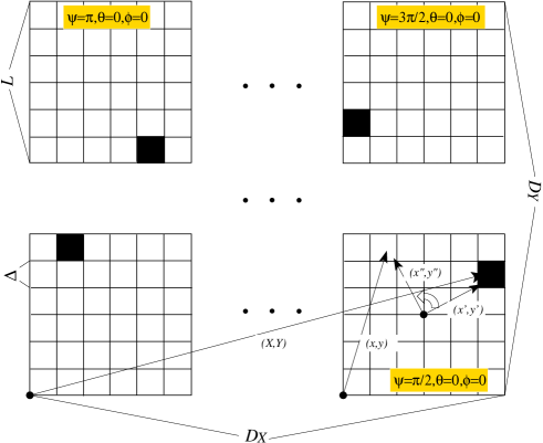
Figure 10: 2D-scheme for the realization of random magnetic fields. The sizes of the box and the cube are $L$ and $\Delta$, respectively. These boxes cover a region of $D_{X}\times D_{Y}$. The Euler angles, by which the boxes are rotated from the lower left box, are indicated. The shaded box marks the same cube after rotation.

To calculate the random magnetic field in any position ($X$, $Y$, $Z$) in the Galaxy $b(X,\,Y,\,Z)$, the following procedure is executed (Fig. 10),

1. transform $(X,\,Y,\,Z)$ to $(x^{\prime},\,y^{\prime},\,z^{\prime})$ as,

   $$x^{\prime}=\frac{X}{L}-i_{x}L-\frac{L}{2},\,y^{\prime}=\frac{Y}{L}-i_{y}L-\frac{L}{2},\,z^{\prime}=\frac{Z}{L}-i_{z}L-\frac{L}{2}$$ (10)

   where $i_{x}={\rm int}(X/L)$, $i_{y}={\rm int}(Y/L)$ and $i_{z}={\rm int}(Z/L)$ are the integer part.

2. rotate $(x^{\prime},\,y^{\prime},\,z^{\prime})$ by Euler angles $(\psi,\,\theta,\,\phi)$ around the centre of the box to get $(x^{\prime\prime},\,y^{\prime\prime},\,z^{\prime\prime})$ as,

   $$\left[\begin{array}[]{c}x^{\prime\prime}\\[4.2679pt] y^{\prime\prime}\\[4.2679pt] z^{\prime\prime}\end{array}\right]=\mathbf{B}\mathbf{C}\mathbf{D}\left[\begin{array}[]{c}x^{\prime}\\[4.2679pt] y^{\prime}\\[4.2679pt] z^{\prime}\end{array}\right]$$ (11)

   and

   $$\mathbf{B}=\left[\begin{array}[]{ccc}\cos\psi&\sin\psi&0\\[4.2679pt] -\sin\psi&\cos\psi&0\\[4.2679pt] 0&0&1\end{array}\right]$$ (12)

   $$\mathbf{C}=\left[\begin{array}[]{ccc}1&0&0\\[4.2679pt] 0&\cos\theta&\sin\theta\\[4.2679pt] 0&-\sin\theta&\cos\theta\end{array}\right]$$ (13)

   $$\mathbf{D}=\left[\begin{array}[]{ccc}\cos\phi&\sin\phi&0\\[4.2679pt] -\sin\phi&\cos\phi&0\\[4.2679pt] 0&0&1\end{array}\right]$$ (14)

   Here the Euler angles are obtained as,

   $$\phi=\left\{\begin{array}[]{lcr@{\leq\mathcal{R}_1\!\!<}l}0&&0\leq\mathcal{R}_{1&0.25\\[4.2679pt] \frac{\pi}{2}&&0.25\leq\mathcal{R}_{1&0.5\\[4.2679pt] \pi&&0.5\leq\mathcal{R}_{1&0.75\\[4.2679pt] \frac{3\pi}{2}&&0.75\leq\mathcal{R}_{1&1\end{array}\right.,}}}}$$ (15)

   $$\theta=\left\{\begin{array}[]{lcr@{\leq\mathcal{R}_2\!\!<}l}0&&0\leq\mathcal{R}_{2&0.33\\[4.2679pt] \frac{\pi}{2}&&0.33\leq\mathcal{R}_{2&0.67\\[4.2679pt] \pi&&0.67\leq\mathcal{R}_{2&1\end{array}\right.,}}}$$ (16)

   and

   $$\psi=\left\{\begin{array}[]{lcr@{\leq\mathcal{R}_3\!\!<}l}0&&0\leq\mathcal{R}_{3&0.25\\[4.2679pt] \frac{\pi}{2}&&0.25\leq\mathcal{R}_{3&0.5\\[4.2679pt] \pi&&0.5\leq\mathcal{R}_{3&0.75\\[4.2679pt] \frac{3\pi}{2}&&0.75\leq\mathcal{R}_{3&1\end{array}\right..}}}}$$ (17)

   Here we use three random numbers $\mathcal{R}_{1}$, $\mathcal{R}_{2}$, and $\mathcal{R}_{3}$ to determine the Euler angles. For simplicity the Euler angles are set to be integer multiple of $\pi/2$ to avoid complex projections.

3. transform $(x^{\prime\prime},\,y^{\prime\prime},\,z^{\prime\prime})$ to $(x,\,y,\,z)$ then to $(l^{\prime},\,m^{\prime},\,n^{\prime})$,

   $$x=x^{\prime\prime}+\frac{L}{2},\quad y=y^{\prime\prime}+\frac{L}{2},\quad z=z^{\prime\prime}+\frac{L}{2},$$ (18)

   and

   $$l^{\prime}={\rm int}(\frac{x}{\Delta}),\quad m^{\prime}={\rm int}(\frac{y}{\Delta}),\quad n^{\prime}={\rm int}(\frac{z}{\Delta}).$$ (19)

   Finally $b(X,\,Y,\,Z)=b_{l^{\prime}m^{\prime}n^{\prime}}$.

Appendix B Simulated total intensity and polarization maps

We display the total intensity $I$ maps in Fig. 11, Stokes $U$ maps in Fig. 12, Stokes $Q$ maps in Fig. 13, polarized intensity $PI$ maps in Fig. 14 and polarization angle $PA$ maps in Fig. 15.

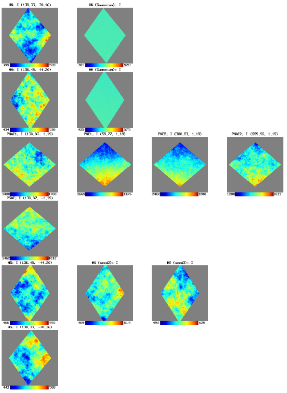
Figure 11: Total intensity $I$ maps for all the simulated patches in gnomonic projection. The centre coordinates are given on top of each panel together with its label (see Table 1 for details). Intensities are in mK brightness temperature at 1.4 GHz. The minimum and maximum of each map is shown together with the wedge below each panel.

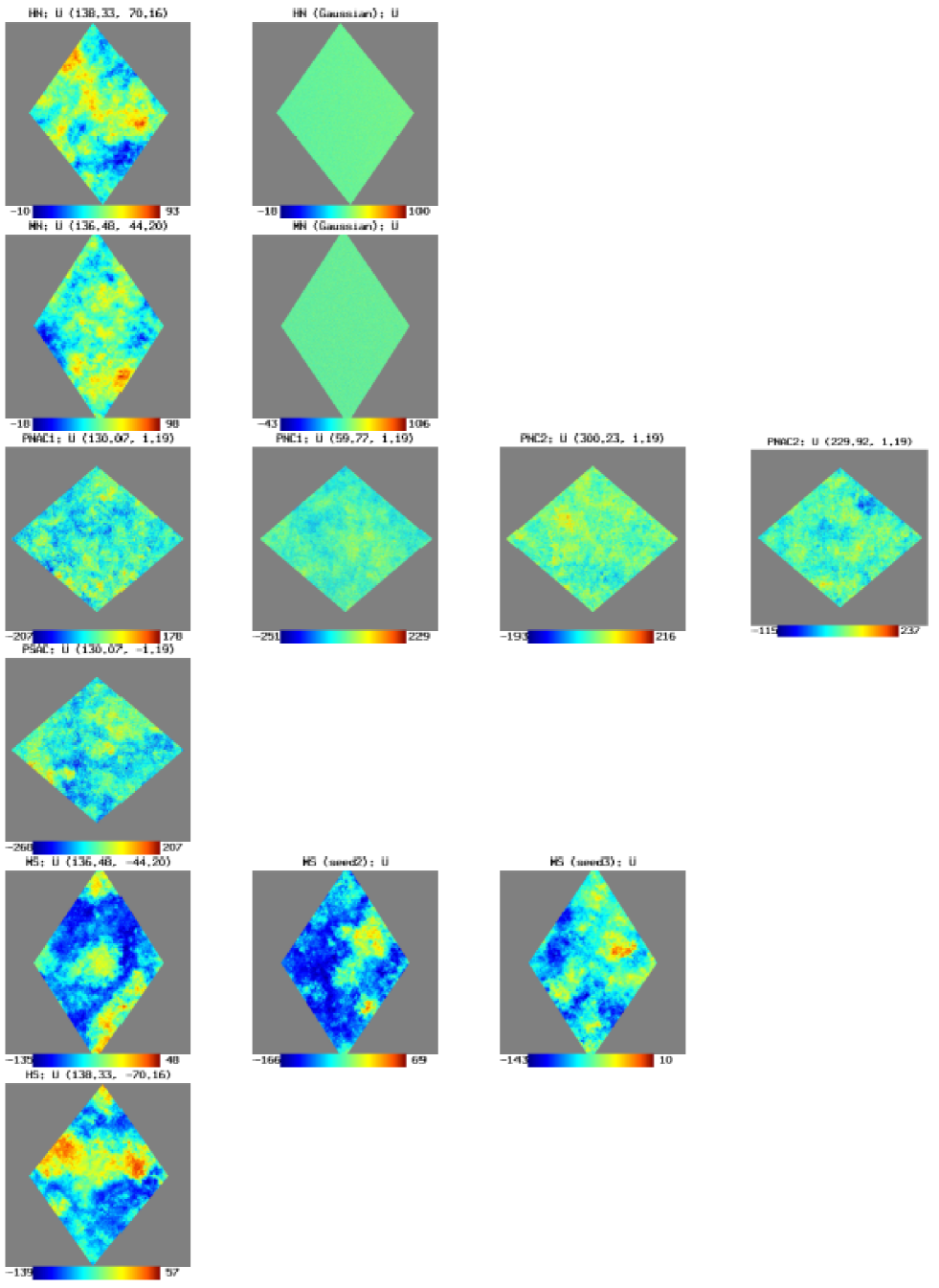
Figure 12: As Fig. 11, but for the simulated Stokes $U$ maps.

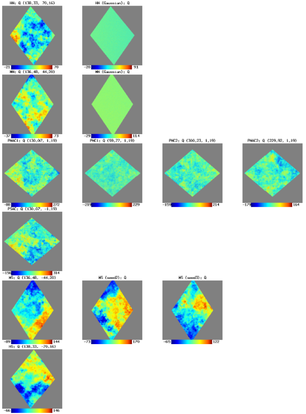
Figure 13: As Fig. 11, but for the simulated Stokes $Q$ maps.

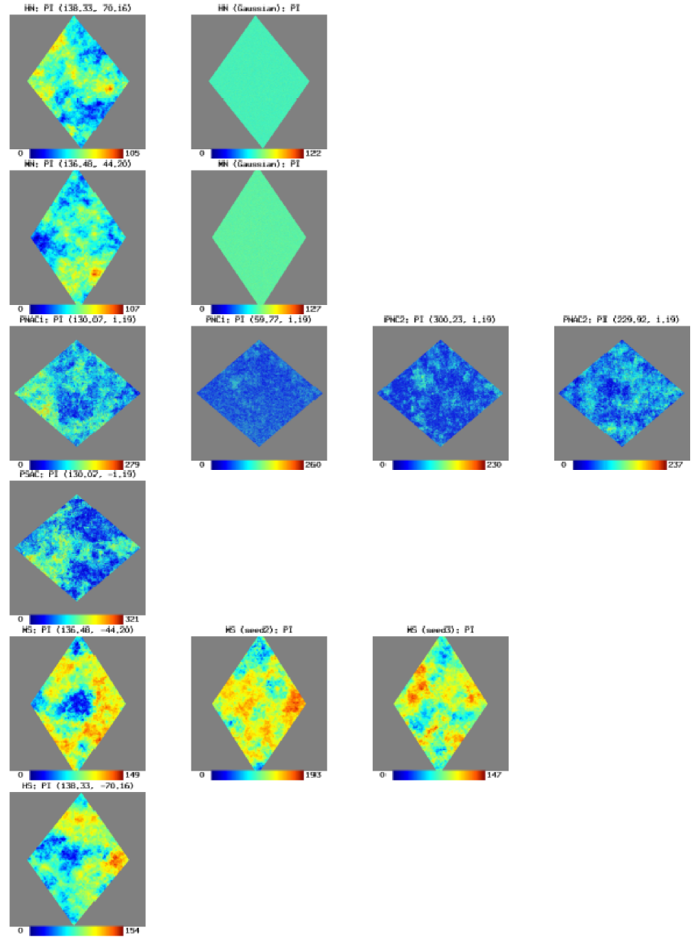
Figure 14: As Fig. 11, but for $PI$ maps calculated from the simulated $U$ and $Q$ maps.

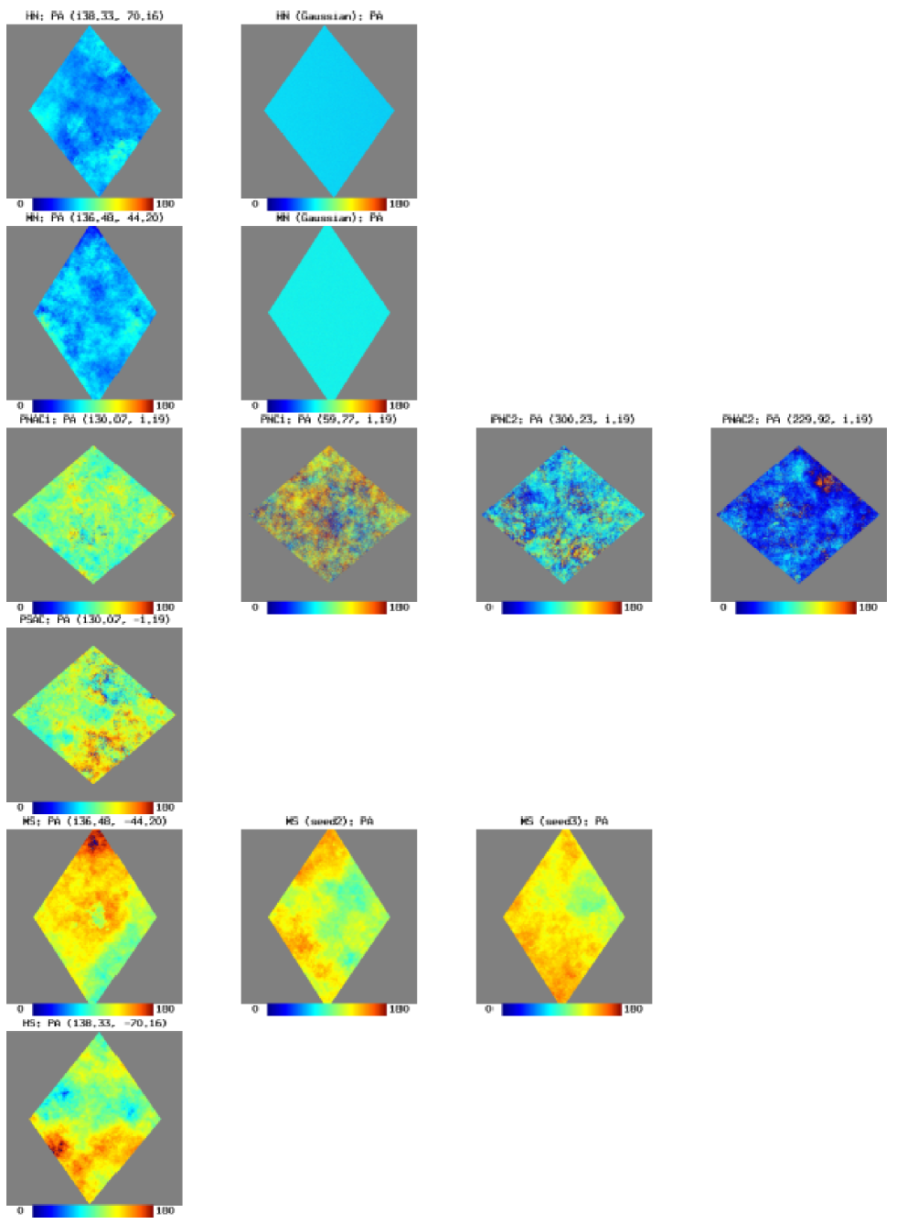
Figure 15: As Fig. 11, but for the polarization angles $PA$ calculated from the simulated $U$ and $Q$ maps.