Static Isotropic Spacetimes with Radially Imperfect Fluids

Abstract

When solving the equations of General Relativity in a symmetric sector, it is natural to consider the same symmetry for the geometry and stress-energy. This implies that for static and isotropic spacetimes, the most general natural stress-energy tensor is a sum of a perfect fluid and a radial imperfect fluid component. In the special situations where the perfect fluid component vanishes or is a spacetime constant, the solutions to Einstein’s equations can be thought of as modified Schwarzschild and Schwarzschild-de Sitter spaces. Exact solutions of this type are derived and it is shown that whereas deviations from the unmodified solutions can be made small, among the manifestations of the imperfect fluid component is a shift in angular momentum scaling for orbiting test-bodies at large radius. Based on this effect, the question of whether the imperfect fluid component can feasibly describe dark matter phenomenology is addressed.

1 Introduction

The observed Universe is homogenous at very large scales but not at small ones where it contains numerous localized matter sources. Within the well-tested [1] theory of General Relativity [2], this means the geometry on large scales can be described by a metric of the Friedman-Robertson-Walker type while at smaller scales it must be approximated by metrics of the Schwarzschild or Schwarzschild-de Sitter forms. These idealized metrics can be derived from the equations of motion of General Relativity by assuming different symmetries at the different scales.

It may be argued that when solving the equations of motion of General Relativity in some symmetric sector, it is natural to consider the same symmetry for the geometry $g_{\mu\nu}$ and stress-energy $T_{\mu\nu}$ to which the geometry couples. Accordingly, when assuming spatial homogeneity for the geometry, it is natural to take $T_{\mu\nu}$ to contain one free function associated with the time direction and one free function associated with the spatial directions. A stress-tensor of this kind is said to be in perfect fluid form and can be written as

$$T^{pf}_{\mu\nu}=(\rho+p)U_{\mu}U_{\nu}+p\,g_{\mu\nu}$$ (1)

with $U^{\mu}$ a unit time-like vector, and $\rho$ and $p$ some functions called the energy density and pressure, respectively. In contrast, for static isotropic geometries, what is natural for $T_{\mu\nu}$ is that it should have three independent functions - two associated with the time and radial directions, and one associated with the remaining two angular directions. A stress tensor of this type can be written as

$$T_{\mu\nu}=T_{\mu\nu}^{pf}+qV_{\mu}V_{\nu}$$ (2)

where the first term on the right hand side is of perfect fluid form (1), and in the second term $V^{\mu}$ is a unit vector pointing in the radial direction and $q$ is some function. Since the modification to the perfect fluid form comes only in the radial components of $T_{\mu\nu}$, a stress-energy tensor of this type may be called radially imperfect. In other terminology it may be said to contain viscous shear. It is the most general stress-energy tensor compatible with staticity and isotropy [3].

In principle, the stress-energy tensor can be calculated in any theory of matter coupled to gravity given a description of the matter distribution. Recently, Cox, Mannheim, and O’Brien performed calculations of this kind assuming a matter component in the form of an incoherent collection of modes of a free (minimally-coupled) massless scalar field [4]. Reproducing earlier results [5], they showed that such a matter distribution puts the stress-energy tensor into the perfect fluid form when the background spacetime is Minkowski. Crucially, however, they also showed that the incoherent collection of field modes does not necessarily generate a perfect fluid stress-energy tensor if the background spacetime is nonhomogenous. In one analytic calculation involving a special static isotropic background, they put the stress-energy tensor into the form (2) and explicitly wrote the functional form for $\rho$, $p$ and $q$ with $q\neq 0$. This corroborates the motivation for using the general form (2) for the stress-tensor source when it is coupled to a static and isotropic geometry.

The calculations in [4] were done in the spirit of field theory on curved spacetime. That is, the background spacetime was assumed to be fixed. The approach was useful because it allowed those authors to determine the field modes explicitly, sum over them, and thus obtain the stress-energy tensor. From the nonperturbative point of view, however, it is important to take into account backreaction, i.e. to obtain a consistent solution to Einstein equations with an imperfect fluid source. The observations in [4] are a direct motivation for doing exactly that.

The purpose of the present work is to study static and isotropic spacetimes coupled with the imperfect fluid stress-energy tensor (2). A similar task has been attempted in [3] but the issue is revisited here in more detail. Attention is focused on describing spacetimes in which the imperfect fluid component is nonvanishing and comparing them to known solutions, like Schwarzschild, in which this component is exactly zero.

Section 2 deals with Einstein’s equations for static and isotropic spacetimes coupled to certain fluids of the form (2). Although isotropy may in some systems also be thought to be an emergent property due to matter coupling [6, 7], in this work it is imposed strongly. Several solutions – modifications of the Schwarzschild, anti-de Sitter, and Schwarzschild-de Sitter spaces – are derived and their properties are discussed. Then, some phenomenological aspects of the modified black-hole solution are studied in Sec. 3. Since one aspect of the phenomenology is similar to that attributed to dark-matter in galaxies, Sec. 4 explores whether the imperfect fluid component can actually be considered a candidate description for dark matter. A brief summary of the results appears in Sec.4.

2 Static Isotropic Solutions

In units where the speed of light and the Newton constant are set to one, the equations of motion of General Relativity are

$$G_{\mu\nu}=8\pi T_{\mu\nu}$$ (3)

with $G_{\mu\nu}$ the Einstein tensor derived from a metric $g_{\mu\nu}$, and $T_{\mu\nu}$ the stress-energy tensor of matter [2]. This section deals with solutions to these equations under the assumption that the geometry is static and isotropic (spherically-symmetric) and the stress tensor is in the radially-imperfect form (2).

With the assumed symmetries, the line element $ds^{2}=g_{\mu\nu}\,dx^{\mu}\,dx^{\nu}$ associated with a metric $g_{\mu\nu}$ in coordinates $x^{\mu}$ can be written as

$$ds^{2}=-f^{2}\,dt^{2}+h^{-1}\,dr^{2}+r^{2}\,d\Omega^{2}$$ (4)

so that the only unfixed components of the metric are $g_{tt}=-f^{2}$ and $g_{rr}=h^{-1}$. The functions $f$ and $h$ depend on the radial coordinate $r$ only and $d\Omega^{2}=d\theta^{2}+\sin^{2}\theta\,d\phi^{2}$ is the line element of a unit sphere. With this choice of coordinates and parametrization, the nonzero components of the Einstein tensor occur only on the diagonal and are

$$G_{tt} =\frac{f^{2}}{r^{2}}\left(1-h-rh^{\prime}\right)$$ (5a)

$$G_{rr} =\frac{1}{r^{2}hf}\left(hf-f+2rhf^{\prime}\right)$$ (5b)

$$G_{\theta\theta} =\frac{r}{2f}\left(2h\left(f^{\prime}+rf^{\prime\prime}\right)+h^{\prime}\left(f+rf^{\prime}\right)\right)$$ (5c)

$$G_{\phi\phi} =\sin^{2}\theta\,G_{\theta\theta}.$$ (5d)

With a radially imperfect fluid of the form (2), the equations of motion become

$$G_{tt} =\rho\,f^{2},$$ (6a)

$$G_{rr} =(p+q)\,h^{-1},$$ (6b)

$$G_{\theta\theta} =p\,r^{2},$$ (6c)

$$G_{\phi\phi} =p\,r^{2}\sin^{2}\theta,$$ (6d)

where $\rho,$ $p$ and $q$ are functions only of $r$, and factors of $8\pi$ have been absorbed on the right hand side. Since equations (6d) and (6c) are multiples of each other, there are actually only three independent equations. And since there are five unknown functions, the equations cannot be solved without specifying additional data. If the geometry, i.e. the functions $f$ and $h$, is specified then the equations can be solved directly to yield the compatible $\rho$, $p$ and $q$. In this way, any spacetime whatsoever can be obtained by some choices for the stress-energy tensor. But it is more constructive to specify reasonable sources, i.e. $\rho$, $p$ and $q$, and subsequently solve for the compatible geometry. Below are a few cases characterized by idealized choices for the energy density $\rho$ and pressure $p$.

2.1 Exactly Vanishing Perfect Fluid

The case of the vanishing perfect fluid is defined by

$$\rho=p=0$$ (7)

everywhere. In this case, equation (6a) can first be solved for $h$. Next, the solution for $h$ can be inserted into (6c) to yield a linear equation for $f$. The results are

$$h =1-\frac{b}{r}$$ (8)

$$f =a\left(\sqrt{1-\frac{b}{r}}\right)-c\left(1-\sqrt{1-\frac{b}{r}}\,\mathrm{log}\left(\frac{\sqrt{r}+\sqrt{r-b}}{\sqrt{d}}\right)\right)$$ (9)

where $a,b,c,d$ are constants. $a$ and $c$ are dimensionless, while $b$ and $d$ have units of length. (The constant $c$ should not be confused with the speed of light which is set to one throughout by a choice of units.) These functions $f$ and $h$ determine the metric. When they are inserted into (6b), they determine the imperfect fluid component to be

$$q=\frac{c}{r^{2}f}.$$ (10)

If the imperfect fluid component is required to vanish, then the constant $c$ must be set to zero. When $h$ in (8) and $f$ in (9) with $c=0$ are inserted into (4), they yield the Schwarzschild line-element with an additional numeric constant $a^{2}$ in front of the $dt^{2}$ component. Because of reparametrization invariance, this constant can be set to unity without loss of generality. Thus the standard black hole solution, with a horizon at the Schwarzschild radius $r=b$ and a singularity at $r=0$, is recovered.

If $c\neq 0$, the coefficient of $dr^{2}$ in the line element remains identical as in the Schwarzschild spacetime. In this sense the quantity $b$ may still be called the Schwarzschild radius. The coefficient of $dt^{2}$ in the line element, however, is for $c\neq 0$ very different than before. This can be seen in Fig. 1 where it is plotted for a few combinations of parameters. A number of new properties are worth pointing out.

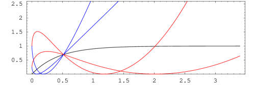
Figure 1: Spacetimes with black-holes. All curves have $a=1$ and $d=b$.

First, the functions $f^{2}$ have a root at a finite radius that is different from the usual $r=b$. Because of the dependence of $q$ on $f$, the imperfect fluid component diverges at those roots. The curvature scalar $R_{\mu\nu\lambda\sigma}R^{\mu\nu\lambda\sigma}$ also diverges there and so these points (actually, surfaces of spheres) are likely unphysical features of the solutions. Their location moves close to $r=b$ as $c$ approaches zero through positive values, and away from $r=b$ as $c$ approaches zero through negative values. If the purpose of the spacetime is to describe behavior outside the black hole, positive $c$ should probably be preferred.

Second, the solutions are only valid for $r>b$ and it is not clear whether they can be extended to $r<b$. Moreover, the quantity $f^{2}$ is not zero at $r=b$ so even if the solution is continued to smaller values of $r$ the spacetime signature may change. Although $r=b$ is always “hidden” behind the singularity described above, this is nonetheless an unphysical feature that suggests that the spacetime should only be studied far from $r=b$.

Third, for large $r$, the functions diverge rather than approach a constant and so they do not describe asymptotically flat spacetimes. This occurs even though the nonvanishing component of the stress-energy tensor, proportional to $q$, falls to zero as $r\rightarrow\infty.$ This is yet another undesirable feature because it implies that the spacetime, even though it is a modification of Schwarzschild space, does not have a limit in which it reproduces Newtonian physics.

As a special case, it is possible to consider the solution with $b=0$. In the Schwarzschild solution, this implies removing the black hole from the spacetime leaving only flat space. In the case with $c\neq 0$, setting $b=0$ gives

$$f\rightarrow a-c+c\,\mathrm{log}\,\sqrt{\frac{4r}{d}}.$$ (11)

While this is valid for all $r>0$, the other two features of the modified black hole spacetimes mentioned above persist. Namely, the function has a root at some finite value of $r$ where the stress-energy tensor component $q$ as well as the scalar curvature $R_{\mu\nu\lambda\sigma}R^{\mu\nu\lambda\sigma}$ diverge, and it does not asymptote to a constant for large $r$. Thus, the resulting spacetime represents quite a drastic departure from Minkowski spacetime and should be interpreted similarly as above.

2.2 Cosmological Constant

The case of the cosmological constant is defined by a perfect fluid with

$$\rho=-p=\Lambda,$$ (12)

where $\Lambda$ is a nonzero spacetime constant. The strategy for obtaining solutions in this case is the same as before. Equation (6a) can first be solved for $h$ to give

$$h=1-\frac{b}{r}-\frac{\Lambda r^{2}}{3}$$ (13)

with $b$ a constant. Then, this can be substituted into (6c) to give a linear equation for $f$,

$$2r^{2}\left(3b-3r+\Lambda r^{3}\right)f^{\prime\prime}+r\left(3b-6r+4\Lambda r^{3}\right)f^{\prime}-\left(3b+4\Lambda r^{3}\right)f=0.$$ (14)

In the special case $b=0$ and $\Lambda<0$, the solution to (14) can be found analytically and then inserted into (6b) to give $q$. The result is

$$f =a\left(\sqrt{1-\frac{\Lambda r^{2}}{3}}\right)+\frac{c}{2}\left(1-\sqrt{1-\frac{\Lambda r^{2}}{3}}\,\mathrm{arctanh}\left(\sqrt{1-\frac{\Lambda r^{2}}{3}}\right)^{-1}\right),$$ (15)

$$q\! =\frac{c}{r^{2}f},$$ (16)

with $a$ and $c$ constants.

The effect of the imperfect fluid can again be removed by setting $c=0$. The resultant function $f$ with $c=0$ and $a=1$ set by convention, when inserted into the line-element ansatz, together with (13) with $b=0$, gives anti-de Sitter spacetime. This is actually a homogenous, rather than only isotropic, space because $b=0$.

If $c\neq 0$, the solution describes a departure from anti-de Sitter. Figure 2 shows the quantity $f^{2}=-g_{tt}$ for a few choices of parameters. For $c>0$, the curves have a root at some finite radius where $q$ and the curvature invariant $R_{\mu\nu\lambda\sigma}R^{\mu\nu\lambda\sigma}$ diverge. Curves with $c<0$ are nonsingular everywhere. For both signs, the curves significantly differ from the anti-de Sitter curve ($c=0$) near $r=0$ but track it closely for $r\rightarrow\infty$. The modified spacetimes are thus asymptotically anti-de Sitter.

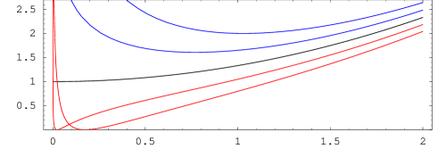
Figure 2: Spacetimes with negative cosmological constant. All curves have $a=1$ and $\Lambda<0$.

For $\Lambda>0$, it can be checked that the function

$$f_{SdS}=h^{1/2}=\sqrt{1-\frac{b}{r}-\frac{\Lambda r^{2}}{3}}$$ (17)

is a solution to (14) and corresponds to $q=0$. It describes Schwarzschild-de Sitter spacetime if $b\neq 0$ and a de Sitter spacetime if $b=0$. A feature of these spaces is that they contain a cosmological horizon at a radius $r_{c}$ for which $f_{SdS}(r_{c})=0$. The metric ansatz in static coordinates suffers from a coordinate singularity at this radius as both $g_{tt}$ and $g_{rr}$ change sign and $g_{rr}$ diverges. Because of this solutions must be specified separately for regions inside and outside the cosmological horizon. While this is not a serious hurdle when $q=0$, it does complicate matters when $q\neq 0$. For example, (15) and (16) can be used for $\Lambda>0$ and $b=0$ to describe solutions outside the horizon but they cannot be used in the region inside the horizon because $f^{2}$ is not real-valued everywhere there for any choice of parameters $a$ and $c$. A solution inside the horizon does exist - it can be computed numerically given some boundary data - but it is not described by (15) and (16).

At this stage, it is worth noting that the function $q$ in (10) and (16) has the same form in two inequivalent situations. It seems reasonable therefore to guess that this form is also valid in the more general case for $\Lambda>0$ and $b\neq 0$. With this guess, the general solution for $f$ can be obtained by solving equation (6b) and then verified by substitution into (6c) and (14). The guess works and the result is

$$f =a\sqrt{1-\frac{b}{r}-\frac{\Lambda r^{2}}{3}}-cf_{c,\Lambda,b}$$ (18)

$$q =\frac{c}{r^{2}f}$$ (19)

where $f_{c,\Lambda,b}$ is a function that can be written analytically but has a complicated form that does not provide insightful information.

Fig. 3 shows $f^{2}=-g_{tt}$ obtained using (18) with various parameters. All curves are plotted in the domain of $r$ between the two horizons of the Schwarzschild-de Sitter solution. Some of the features that distinguish them from the Schwarzschild-de Sitter case are qualitatively similar to those already found in the modified Schwarzschild spacetimes ($\Lambda=0$).

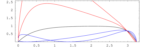
Figure 3: Spacetimes with black-holes and cosmological constant. All curves have $\Lambda b^{2}=10^{-6}$ and $a=1$.

First, all curves with $c\neq 0$ have zeros at radii that are different from the black-hole and cosmological horizons in the unmodified spacetime. The curvature invariant $R_{\mu\nu\lambda\sigma}R^{\mu\nu\lambda\sigma}$ diverge at those zeros. Their location moves close to the black-hole horizon as $c$ approaches zero through positive values, and move close to the cosmological horizon as $c$ approaches zero through negative values.

Second, for $c\neq 0$, the curves do not fall to zero at the black hole or cosmological horizons. This poses problems with signature change.

Third, the maxima of the curves with $c\neq 0$ are shifted relative to the $c=0$ case. For $c>0$, the maximum occurs closer to the cosmological horizon. For $c<0$, it occurs closer to the black-hole horizon.

2.3 Almost-Constant Perfect Fluid

This case summarizes and elaborates on the discussion in [3]. It involves a more qualitative description of the effect of the imperfect fluid component on geometry when the assumption that $\rho$ and $p$ be strict spacetime constants is relaxed. The profiles for $\rho$, $p$ and $q$ are assumed to satisfy

$$\rho =\left\{\begin{array}[]{ll}\rho(r)&\mbox{for}\;\;r<R_{\rho}\\ \Lambda&\mbox{for}\;\;r\geq R_{\rho}\end{array}\right.$$ (20c)

$$p =\left\{\begin{array}[]{ll}p(r)&\mbox{for}\;\;r<R_{p}\\ -\Lambda&\mbox{for}\;\;r\geq R_{p}\end{array}\right.$$ (20f)

$$q =\left\{\begin{array}[]{ll}q(r)&\mbox{for}\;\;r<R_{q}\\ 0&\mbox{for}\;\;r\geq R_{q}\end{array}\right.$$ (20i)

with appropriate continuity conditions at $r=R_{\rho},R_{p},R_{q}$. The boundary radii define compact regions where the corresponding stress-energy tensor components differ from constants. A cosmological constant is allowed for large $r$ in the profiles for $\rho$ and $p$ but not for $q$.

When (20c) is inserted into (6a), the resulting equation can be solved in the region $r>R_{\rho}$ to give the solution

$$h=1-\frac{b}{r}-\frac{\Lambda r^{2}}{3}\qquad\mbox{for}\quad r>R_{\rho}.$$ (21)

This can then be inserted into (6b) and (6c). The results that ensue depend on the relative sizes of $R_{\rho}$, $R_{p}$ and $R_{q}$. There are six possible orderings and these can be treated exhaustively.

In general, the strategy for obtaining exact solutions is to solve (6c) for $r>R_{\rho}$ and $r>R_{p}$ where the details of the $\rho$ and $p$ profiles are not important. The equation, and therefore the solution, in this region are equivalent to that studied in the previous sections. When the solution is inserted into (6b), the necessary form for $q$ is obtained and it is not a function with compact support as required by (20i). To be consistent, then, it is necessary to require that $q=0$ in that region. Thus, the exterior solution becomes

$$f=a\sqrt{h}\qquad\mbox{for}\quad r>R_{\rho},\;\;r>R_{p}.$$ (22)

The pathologies associated with large radii described for the idealized solutions in Sec. 2.1 and 2.2 are thus removed.

An interesting case is when $R_{p}=R_{q}>R_{\rho}$, illustrated in Fig. 4. As in the general case, the solution in the exterior region $r>R_{p}$ reduces to (22). However, in this case there is a shell $R_{\rho}<r<R_{p}$ where

$$f\neq a\sqrt{h}.$$ (23)

This general feature may also be argued to hold in regions $r<R_{\rho}$ where $q\neq 0$ [8].

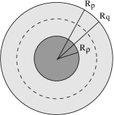
Figure 4: Isotropic spacetime with $\rho$, $p$ and $q$ profiles with compact support.

The precise form of $f$ in the shell $R_{\rho}<r<R_{p}$ depends on the pressure profile $p$. Under certain conditions, however, it may be reasonable to approximate $f$ using (9) or (18) when $p$ does not differ significantly from a constant. This can only be done in a region from $r=R_{\rho}$ to some intermediate radius shown by the dashed line in Fig. 4. Beyond this intermediate radius, the pressure must differ sufficiently from a constant in order to ensure that $f$ goes to (22) for $r>R_{p}$.

3 Phenomenology

The most interesting among the solutions with imperfect fluids is the modified black hole spacetime with compact source of Sec. 2.3. However, that solution cannot be written explicitly without assuming profiles for $\rho$, $p$ and $q$. In contrast, the modified black hole spacetime of Sec. 2.1 can be written down analytically in terms of only two free parameters. Moreover, as argued in Sec. 2.3, it may be a reasonable approximation to the more physical spacetime in a region close to the matter distribution with energy density $\rho$ and away from $r=\infty$ (or $r=r_{c}$ if $\Lambda>0$). So it may be instructive to consider that idealized spacetime as a concise model of the possible effects of a radial imperfect fluid component on geometry. The model does have limitations, however. In particular, it does not easily allow to estimate effects due to multiple source. Bearing such limitations in mind, this section aims to compare the phenomenology of the modified spacetime, following [2], with the Schwarzschild black hole.

The line element of the modified Schwarzschild solution, repeated here for convenience, is

$$ds^{2}=-f^{2}\,dt^{2}+h^{-1}\,dr^{2}+r^{2}\,d\Omega^{2}$$ (24)

with

$$f =a\left(\sqrt{1-\frac{b}{r}}\right)-c\left(1-\sqrt{1-\frac{b}{r}}\,\mathrm{log}\left(\frac{\sqrt{r}+\sqrt{r-b}}{\sqrt{d}}\right)\right)$$ (25)

$$h =1-\frac{b}{r}.$$ (26)

It reduces to that of Schwarzschild spacetime for $a=1$ and $c=0$ and describes modification thereof when $c\neq 0$. In the analysis below, all analytic results are shown with $a$ explicitly present but all numerical quantities are evaluated using a convention setting $a=1$.

3.1 Orbital motion

A unit four-velocity vector $u^{\mu}=dx^{\mu}/d\tau$, where $\tau$ is the proper time, should obey the normalization condition $-1=u_{\mu}u^{\mu}.$ Assuming motion in the plane $\theta=\pi/2$, this condition gives

$$-1=-f^{2}\,\dot{t}^{2}+h^{-1}\,\dot{r}^{2}+r^{2}\,\dot{\phi}^{2}$$ (27)

with the dot denoting $d/d\tau.$ Because $(d/dt)^{\mu}$ and $(d/d\phi)^{\mu}$ are Killing fields of the static isotropic spacetime, the quantities $E=f^{2}\,\dot{t}$ and $L=r^{2}\,\dot{\phi}$, called energy and angular momentum, respectively, are constants of motion. Writing (27) in terms of $E$ and $L$ yields

$$\frac{1}{2}\dot{r}^{2}+V_{eff}=\frac{1}{2}E^{2}$$ (28)

with

$$V_{eff}=\frac{h}{2}\left(1+\frac{L^{2}}{r^{2}}\right)+\frac{1}{2}E^{2}\left(1-\frac{h}{f^{2}}\right).$$ (29)

This is an equation for a test particle moving in one dimension in an effective radial potential $V_{eff}$.

A test particles moving in a circular orbit is at the minimum of the potential and has $dV_{eff}/dr=0.$ Since it does not move radially, it also has $\dot{r}=0$ so that $V_{eff}=E^{2}/2$. Together, these two conditions can be used to solve for $L$ and $E$ in terms of the orbit radius. The general result

$$E^{2} =\frac{f^{3}}{f-rf^{\prime}}\sim a^{2}+ac\,\mathrm{log}\frac{4r}{d}$$ (30)

$$L^{2} =\frac{r^{3}f^{\prime}}{f-rf^{\prime}}\sim\frac{cr^{2}}{2a}+\frac{br}{2}$$ (31)

is independent of the function $h$. The last approximations are obtained after expanding for large $r$ and small $c$ and ignoring all but the leading terms that are either proportional to $c$ or are independent of it.

The general result reproduces the Schwarzschild scalings when $c=0$. For $c\neq 0$, however, the correction terms can dominate for $r$ sufficiently large. In particular, the scaling of angular momentum squared, $L^{2}$, shifts from linear to quadratic near

$$r_{\star}=\left|\frac{ab}{c}\right|.$$ (32)

Since angular momentum $L$ is the product of radius $r$ and velocity $v$, a scaling $L^{2}\propto r^{2}$ implies that the velocity of orbiting particles is independent of distance. Interestingly, this behavior is actually observed within galaxies where it is interpreted either as evidence for the existence of dark matter or as a motivation for modifying the dynamics of general relativity. Phenomenologically, the observed behavior is well-described by the framework of Modified Newtonian Dynamics (MOND) [9, 10] which postulates that orbiting bodies deviate from standard Newtonian behavior and start orbiting at a constant velocity when their acceleration falls below the threshold $10^{-27}m^{-1}$. (And by what seems a coincidence, the acceleration threshold is within an order of magnitude of the root of the observed cosmological constant $\Lambda$.) Setting this equal to the Newtonian expression $b/r^{2}$ implies that the threshold radius in the MOND description is

$$r_{\star\,M\!O\!N\!D}=\left(3\!\cdot\!10^{13}\,m^{1/2}\right)\sqrt{b}.$$ (33)

If the derived threshold (32) is to account for galaxy rotation curves, then, assuming a fixed parameter $a$, the parameter $c$ should depend on $b$ as

$$c=\gamma\sqrt{b}$$ (34)

with $\gamma$ some quantity with units of $m^{-1/2}$. Substituting this relation into (32) and setting that equal to (33) gives

$$\gamma_{M}=3\!\cdot\!10^{-14}\,m^{-1/2}.$$ (35)

The subscript denotes this value is obtained from the MOND phenomenological description.

If the derived threshold (32) is said not to be responsible for galaxy rotation curves, then a bound on $c$ can be formulated from each galaxy’s data. It is convenient to summarize those bounds using the parameter $\gamma$ from (34). Since the size of a galaxy is typically an order of magnitude larger than (33), the bound on $\gamma$ would in this case be about an order of magnitude lower than (35).

Within the solar system, objects orbit the Sun according to the unmodified scaling at least up to radii $50$ times the Earth’s orbit radius. Using $b$ as the Schwarzschild radius of the Sun, these observations yield the bounds

$$|c_{S}|<10^{-10},\qquad|\gamma_{S}|<10^{-13}m^{-1/2}$$ (36)

The subscripts denote that the bound refers to an observation wherein the central massive object is the Sun and the bound on $\gamma$ is presented assuming the scaling (34).

3.2 Perihelion Precession

If a test particle is displaced from a circular orbit, it oscillates around the equilibrium radius with frequency $\omega_{r}$ given by $\omega_{r}^{2}=d^{2}V_{eff}/dr^{2}$ with the right-hand-side evaluated at the orbit radius. Its angular frequency is $\omega_{\phi}=L/r^{2}$ evaluated at the orbit radius. When these are not equal, the object precesses with frequency $\omega_{p}=\omega_{\phi}-\omega_{r}.$ Using the modified black-hole spacetime and evaluating $\omega_{p}$ for large $r$ and small $c$ yields

$$\omega_{p}\sim\frac{3\sqrt{2}\,b^{3/2}}{4\,r^{5/2}}-c\frac{\sqrt{2}}{4\,a\sqrt{br}}$$ (37)

The precession frequency for an elliptic but close to circular orbit differs from this result by a factor of order one [2].

The precession of the planet Mercury around the Sun is consistent with the $c=0$ form of $\omega_{p}$ with an accuracy of $10^{-5}$ [11]. This leads to

$$|c_{S}|<10^{-19},\qquad|\gamma_{S}|<10^{-21}\,m^{-1/2}.$$ (38)

Again, the subscripts denote that the central source is the sun. The bound on $\gamma_{S}$ is obtained using (34).

3.3 Redshift

In the static coordinates of (24), $\xi^{\mu}=(1,0,0,0)^{T}$ is a time-like Killing vector. Its magnitude is $(-\xi_{\mu}\xi^{\mu})^{1/2}=f$ and so a unit four-velocity vector $u^{\mu}$ parallel to $\xi^{\mu}$ can be written as $u^{\mu}=f^{-1}\,\xi^{\mu}.$ The frequency $\omega$ of a light ray with momentum vector $k^{\mu}$ recorded by an observer with four-velocity $u^{\mu}$ is $\omega=k_{\mu}u^{\mu}=f^{-1}\,k_{\mu}\xi^{\mu}.$ If two observers with unit four-velocity located at two different locations labeled by radii $r_{1}$ and $r_{2}$ measure frequencies $\omega_{1}$ and $\omega_{2}$ for the same light ray, the ratio of their results is then

$$\frac{\omega_{1}}{\omega_{2}}=\frac{f(r_{2})}{f(r_{1})}.$$ (39)

Without loss of generality, the coordinate $r_{2}$ can be replaced by $r_{2}=r_{1}(1+\delta)$ for some $\delta\geq-1$.

It is convenient to also define a quantity

$$Y=\frac{\omega_{2}-\omega_{1}}{\omega_{2}}=1-\frac{\omega_{1}}{\omega_{2}}$$ (40)

that measures the relative change in the measured frequencies. This can be computed in the limit of large $r_{1}$, small $c$ and small $\delta$ to yield

$$Y\sim-\frac{b\delta}{2r}-\frac{c\delta}{2a}$$ (41)

after omitting terms of order $c^{2}$, $r^{-2}$, $\delta^{2}$, $c/r$, and higher.

In Earth-based redshift experiments, the accuracy with which observations match (41) with $c=0$ is $7\!\cdot\!10^{-5}$ [12]. This gives

$$|c_{E}|<10^{-15},\qquad|\gamma_{E}|<10^{-12}\,m^{-1/2},$$ (42)

where the subscripts indicate the result refers to an Earth-based observation.

4 Discussion

In a generic theory of the universe, the matter field content can be split into standard-model fields $\psi$, a scalar field $\varphi$, and other fields $\chi$ thought to describe dark matter. Each of these fields can in principle give rise to a stress-energy tensor with an imperfect fluid component $q$. Sec. 3 shows that the effects of this component in central-mass situations can be made as small as necessary by changing the parameter $c$. The argument from Sec. 2.3 also implies that the imperfect fluid effects can be totally removed at large scales while producing effects near conventional matter sources that are similar to those usually associated with dark-matter. This section thus aims to combine theoretical ideas and phenomenological constraints in order to understand to what extent and under what conditions the imperfect fluid component can account for dark-matter effects and thereby dispense with the need to postulate the existence of separate dark-matter fields $\chi$.

For simplicity, attention can be concentrated on the scalar field $\varphi$. A large class of theories involving such a field have an action of the form

$$S=\int d^{4}x\,\sqrt{-g}\left(\frac{1}{2}g^{\alpha\beta}\partial_{\alpha}\varphi\partial_{\beta}\varphi+V(\varphi)\right),$$ (43)

where $V(\varphi)$ is a potential that does not depend on derivatives of $\varphi$. The stress-energy tensor, obtained by variation with respect to the metric, is

$$T_{\mu\nu}=\partial_{\mu}\varphi\partial_{\nu}\varphi-\frac{1}{2}g_{\mu\nu}g^{\alpha\beta}\partial_{\alpha}\varphi\partial_{\beta}\varphi-g_{\mu\nu}V(\varphi).$$ (44)

For a field configuration with $\partial_{\mu}\varphi=0$, the tensor becomes $T_{\mu\nu}=-g_{\mu\nu}V(\varphi)$ and thus describes a cosmological constant with $\Lambda=V(\varphi)$. On small scales, it is plausible for the field $\varphi$ to respond to the curvature of spacetime around massive objects, break the condition $\partial_{\mu}\varphi=0$ in certain regions, and thus lead the stress-energy tensor to acquire more structure. In static and isotropic regions, the tensor will take the general form (2) with the energy density $\rho$, pressure $p$, and imperfect fluid component $q$ related to the derivatives of the field. In this way, the component $q$ acting like a dark field can become a companion of a conventional energy density $\rho$ [14, 15].

As shown in Sec. 2, the imperfect fluid component $q$ in a static isotropic spacetime takes the form $q\sim c/r^{2}f.$ The quantity $c$ that determines its magnitude is a real dimensionless number and it is not unreasonable for it to actually represent a ratio of physically relevant scales. The dimensionful quantities in the general central source setup of Sec. 2.3 are $\Lambda$, $\rho$, $p$, $R_{\rho}$, $R_{p}$, and $R_{q}$ (henceforth the quantities $\rho$ and $p$ are taken to represent averages of energy density and pressure over the relevant regions of spacetime). The quantity $b$, the Schwarzschild radius of the energy density distribution, is a derived quantity proportional to $\rho R_{\rho}^{3}$. In the situation depicted in Fig. 4, the radii obey $R_{p}\sim R_{q}>R_{q}$ and it is reasonable to assume that $R_{p}$, $R_{q}$ and $p$ are somehow related to $\Lambda$. The independent dimensionful quantities are thus reduced to $\Lambda$, and two of $\rho$, $R_{\rho}$, and $b$.

Other dimensionful parameters may enter from the specific theory describing the field $\varphi$. In a quantum theory, for example, a new dimensionful quantity is the Planck mass $M_{P}$. In an interacting theory, dimensionful parameters may also appear from coupling constants in potentials involving $\varphi$. For simplicity, however, the following arguments assume that these particle-physics parameters are not important.

The most general dimensionless quantity that can be composed of the relevant parameters can then be written as

$$c=\alpha\,b^{n_{b}}\,\Lambda^{n_{\Lambda}}\,\rho^{n_{\rho}}=\beta\,b^{n_{b}}\,\Lambda^{n_{\Lambda}}\,R_{\rho}^{n_{R}}$$ (45)

where $\alpha$ and $\beta$ are real numbers either of order one or with a physical interpretation, and the exponents obey

$$0=n_{b}-2n_{\Lambda}-2n_{\rho}=n_{b}-2n_{\Lambda}+n_{R}.$$ (46)

The discussion of orbital motion in Sec. 3 suggests that the scaling should be $c=\gamma\sqrt{b}$, which corresponds to setting $n_{b}=1/2$.

The value of $\gamma$ appears to be (35) in galaxies but the bound (38) from Mercury perihelion precession indicates that it must be significantly smaller within the solar system. Thus, if $\gamma$ is a universal constant, the perihelion precession observation rules out using the imperfect fluid effect on orbital motion as a description for dark matter leading to flat galaxy rotation curves.

If $\gamma$ is not a universal constant, then the powers $n_{\rho}$ or $n_{R}$ in (45) should be different from zero. If $n_{\Lambda}>1/4$ and $n_{\rho}<0$, the effective value of $c$ can be much different in galaxies and within the solar system. For example, for $n_{\Lambda}=1$, $c$ becomes

$$c=\alpha\,b^{1/2}\,\Lambda\,\rho^{-3/4}=\beta\,b^{1/2}\,\Lambda\,R^{3/2}.$$ (47)

If $\rho\sim\Lambda$ and $\alpha\sim 1$, then $c\sim b^{1/2}\Lambda^{1/4}$ and the boundary between linear and quadratic angular momentum scaling occurs at a radius close to (33). A similar boundary radius can be obtained by taking a larger and more realistic value for $\rho$ for a galaxy and multiplying by a larger number $\alpha$. For a dense system, $\rho\gg\Lambda$, the value of $c$ becomes much smaller and the transition radius (32) correspondingly larger. In this way, the imperfect fluid model with such scaling can be made to account for galaxy rotation curves and also be consistent with all the observational bounds described in Sec. 3.

In principle, the correct scaling should be computed from some theory using (44). Such a computation would be desirable also because it could shed light on how multiple sources affect the strength of the imperfect fluid in realistic mass distributions. However, this requires solving for and manipulating the modes of the field $\varphi$ in the curved background described in Fig. 4, and is not straight-forward. Without the specific theory, the rather special form of the scaling must be regarded only as a phenomenological fit.

If the interpretation of dark matter effects in terms of an imperfect fluid related to $\varphi$ were to hold, it would have a number of consequences. First, it would imply that direct experimental searches for dark matter particles should give results consistent with properties of the field $\varphi$ responsible for the background cosmological constant. Second, the required scaling for the parameter $c$ would imply that the threshold radius $r_{\star}$ should depend on the density or size of a galaxy. This effect may be testable once the imperfect fluid is better understood. Third, it would imply that the pressure component of the field responsible for $q$ cannot be constant everywhere. If it were, the imperfect fluid phenomenology would not be localized around the central source and would be severely inconsistent with large-scale properties of the observed universe.

Other phenomena such as gravitational lensing and structure formation in cosmology [10, 13, 16, 17] may provide more constraints when analyzed in the context of the imperfect fluid. Distinguishing between a dark-matter field source and an imperfect fluid component should be possible because because the two have slightly different signatures: whereas the former affects both the $g_{rr}$ and $g_{tt}$ components of the metric, the imperfect fluid affects primarily $g_{tt}.$ Related issues have been studied in the context of alternative theories of gravity [10, 13].

5 Conclusion

Static and isotropic geometries can be consistently coupled to a stress-energy tensor composed of a perfect fluid component plus a radial imperfect fluid component. In cases where the perfect fluid component vanishes exactly or describes a cosmological constant, the solutions to the Einstein’s equations are modifications of black hole spacetimes. One of such analytic solutions, described in Sec. 2.1, can be thought of as a modification to the Schwarzschild black-hole. Its line element differs from that of Schwarzschild space in the $dt^{2}$ coefficient, which in addition to the Schwarzschild radius $b$ also contains two new parameters: one of these, $c$, is dimensionless; the other, $d$, has dimensions of length or mass. The spacetime contains a curvature singularity at $r>b$ and is not asymptotically flat. Both these properties are pathologies that can be traced to an assumption that the pressure of the perfect fluid component of the stress-energy tensor vanishes exactly, and as discussed in Sec. 2.3, may be removed by relaxing this assumption.

Despite its limitations, the modified Schwarzschild spacetime can nonetheless be useful in describing how a radial imperfect fluid component can affect geometry. If the modified black-hole spacetime is treated as a model for the Earth’s or the Sun’s gravitational field, then, as Sec. 3 shows, various solar system observations constrain the parameter $c$.

Among the deviations from Schwarzschild phenomenology is a shift in scaling of angular momentum $L$ of an orbiting test body from $L^{2}\sim r$ to $L^{2}\sim r^{2}$ at large $r$. Because this kind of behavior is an observed feature in many galaxies and one of the motivations for studies involving dark matter or modified gravitational dynamics, Secs. 3 and 4 discuss conditions under which the imperfect fluid model can be used as a description for dark matter while still being consistent with solar system constraints. The conclusion is that for this to be possible the parameter $c$ must scale with various other quantities in a rather special way. The scaling makes the setup somewhat contrived but also falsifiable.

That a new term in the stress-energy tensor can produce new phenomenology should not in itself be surprising. After all, it is an additional source in the equations of motion and thus affects geometry. The description of dark-matter effects in terms of an imperfect fluid component, however, may be attractive in some regards. For example, if an imperfect fluid component of the correct magnitude were indeed produced by a scalar field $\varphi$ associated with the cosmological constant, it may help understand dark-matter effects without the need to introduce otherwise undetected fields or to modify gravitational interactions. From this perspective, the results from Sec. 4 suggest that the imperfect fluid component may at least be one of several complementary aspects to the wider subject of dark matter. Alternatively, that discussion can be viewed as a set of conditions that an effective theory of a dark-energy field $\varphi$ should satisfy for it not to be at odds with solar-system and galaxy phenomenology.

Acknowledgements

I would like to thank P. Mannheim and S. McGaugh for correspondence.

References

- [1] C. M. Will, Living Rev. Relativity 9, (2006), 3. URL (cited on 09/04/09): http://www.livingreviews.org/lrr-2006-3 .
- [2] R. M. Wald, General Relativity, CUP 1984.
- [3] P. D. Mannheim, Prog. Part. Nucl. Phys. 56, 340 (2006) [arXiv:astro-ph/0505266].
- [4] D. Cox, P. D. Mannheim and J. O’Brien, arXiv:0903.4381 [gr-qc].
- [5] P. D. Mannheim and D. Kazanas, Gen. Rel. Grav. 20, 201 (1988).
- [6] T. Konopka, Phys. Rev. D 79, 085012 (2009) [arXiv:0904.0527 [hep-th]].
- [7] T. Konopka, arXiv:0903.4342 [gr-qc].
- [8] T. Jacobson, Class. Quant. Grav. 24, 5717 (2007) [arXiv:0707.3222 [gr-qc]].
- [9] M. Milgrom, arXiv:0801.3133 [astro-ph].
- [10] R. H. Sanders and S. S. McGaugh, Ann. Rev. Astron. Astrophys. 40, 263 (2002) [arXiv:astro-ph/0204521].
- [11] V. Kagramanova, J. Kunz and C. Lammerzahl, Phys. Lett. B 634, 465 (2006) [arXiv:gr-qc/0602002].
- [12] R. F. C. Vessor et. al., Phys. Rev. Lett. 45, 2081 (1980).
- [13] M. A. Walker, APJ 430, 463-466 (1994).
- [14] Y. Sobouti, arXiv:0810.2198 [gr-qc].
- [15] Y. Sobouti, A. H. Zonoozi and H. Haghi, arXiv:0906.0668 [gr-qc].
- [16] G. Bertone, D. Hooper and J. Silk, Phys. Rept. 405, 279 (2005) [arXiv:hep-ph/0404175].
- [17] D. Clowe, M. Bradac, A. H. Gonzalez, M. Markevitch, S. W. Randall, C. Jones and D. Zaritsky, Astrophys. J. 648, L109 (2006) [arXiv:astro-ph/0608407].